
Dynamic Stress Path under Obliquely Incident P- and SV-Waves
Abstract
:1. Introduction
2. Seismic Dynamic Stress Caused by Obliquely Incident P- and SV-Waves
2.1. Calculation Formulas of Seismic Dynamic Stress
2.2. Characteristics of Dynamic Stress Path
3. Analysis of Factors Influencing the Dynamic Stress Path
3.1. Influence of Poisson’s Ratio and Incident Angle
3.2. Influence of Frequency and Incident Angle
3.3. Influence of Wave Velocity and Incident Angle
3.4. Influence of Phase Difference and Incident Angle
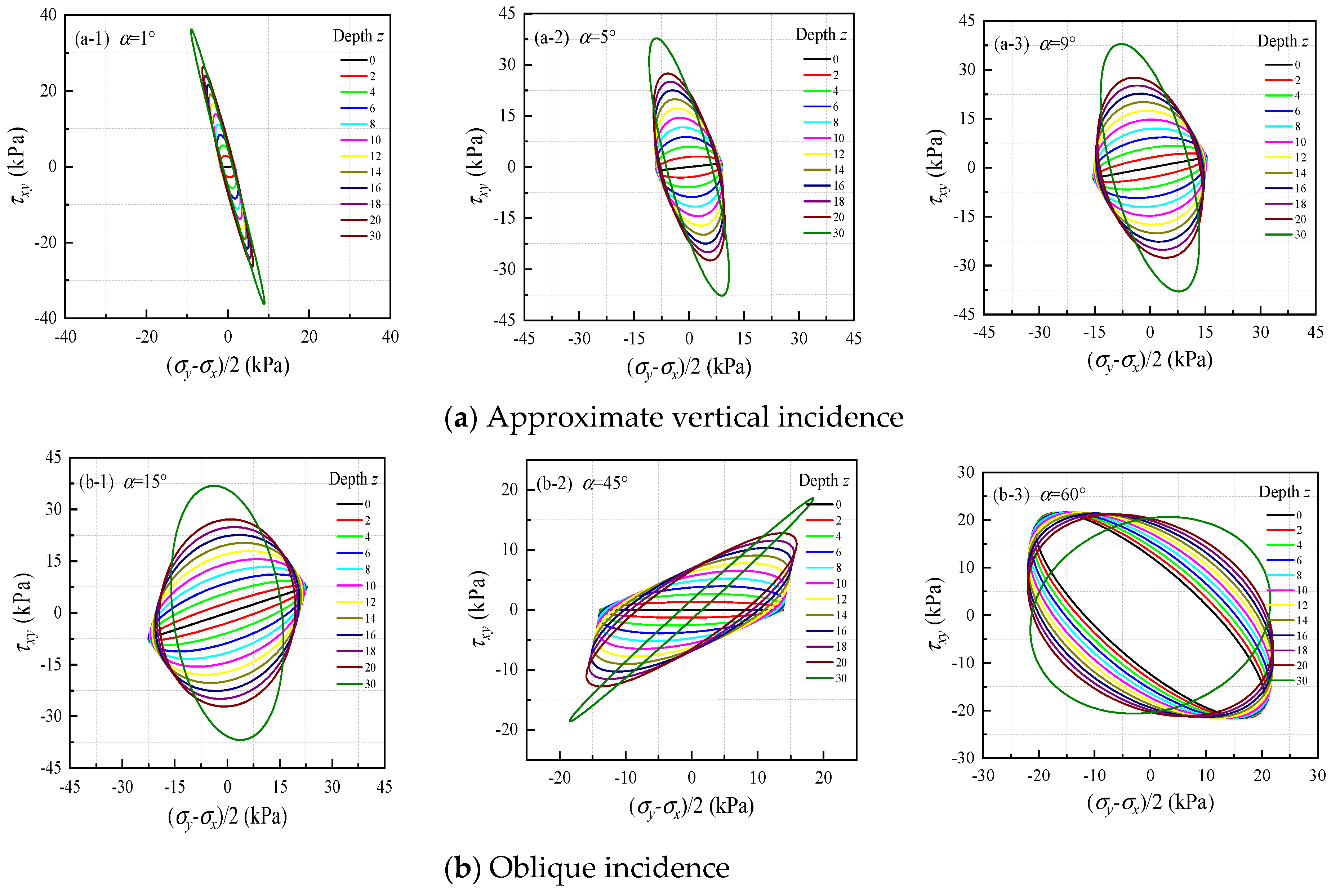
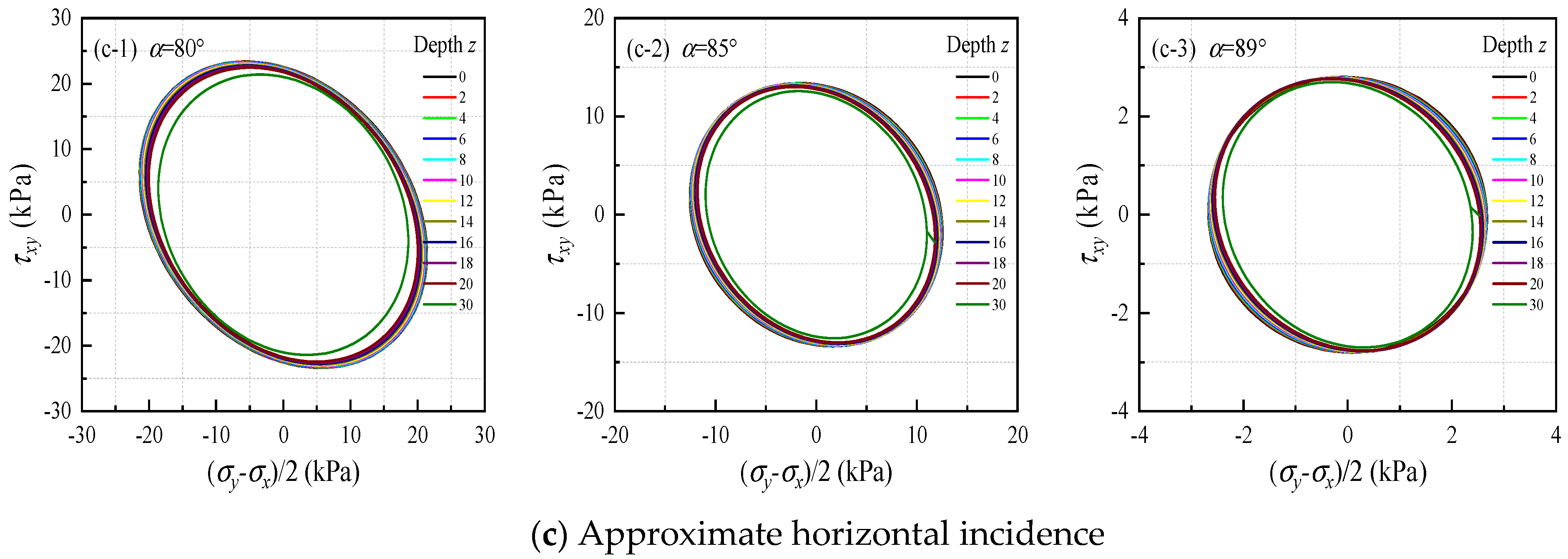
3.5. Influence of Soil Depth and Incident Angle
4. Conclusions
- (1)
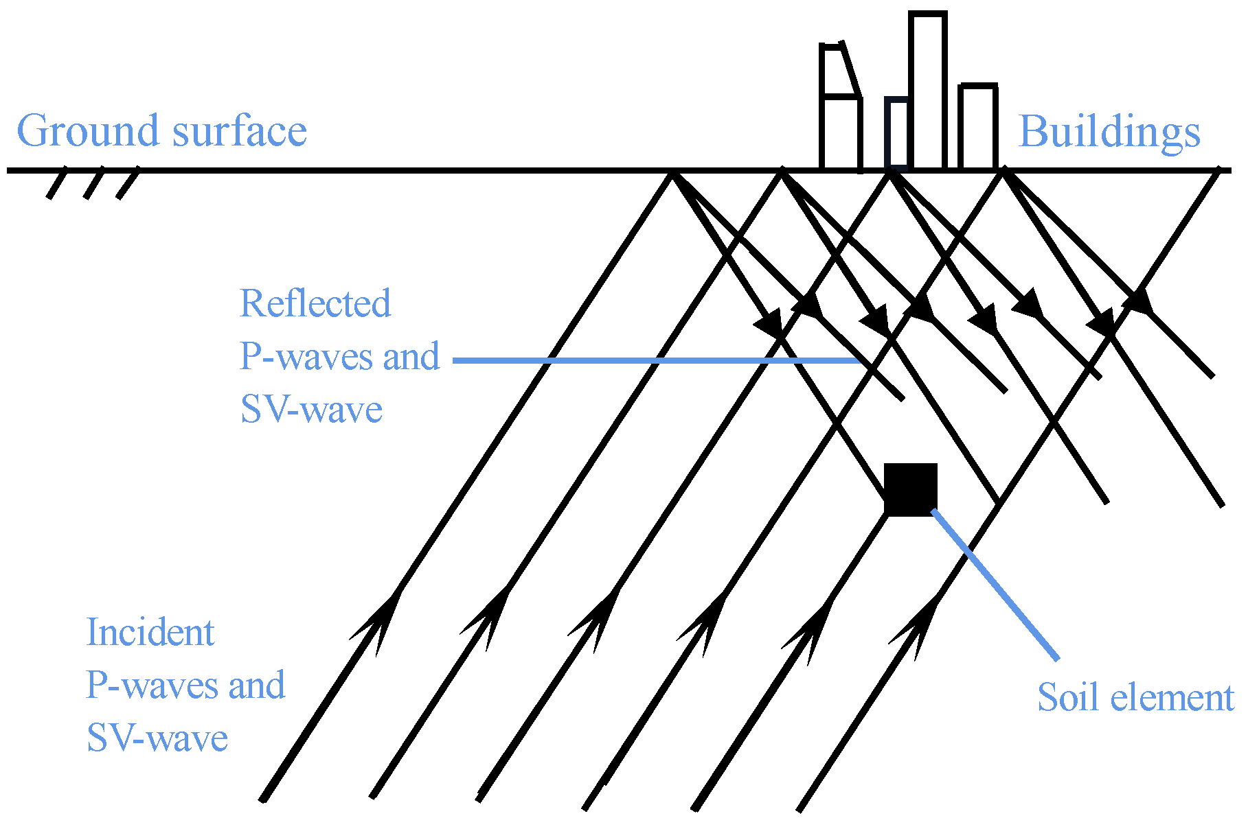
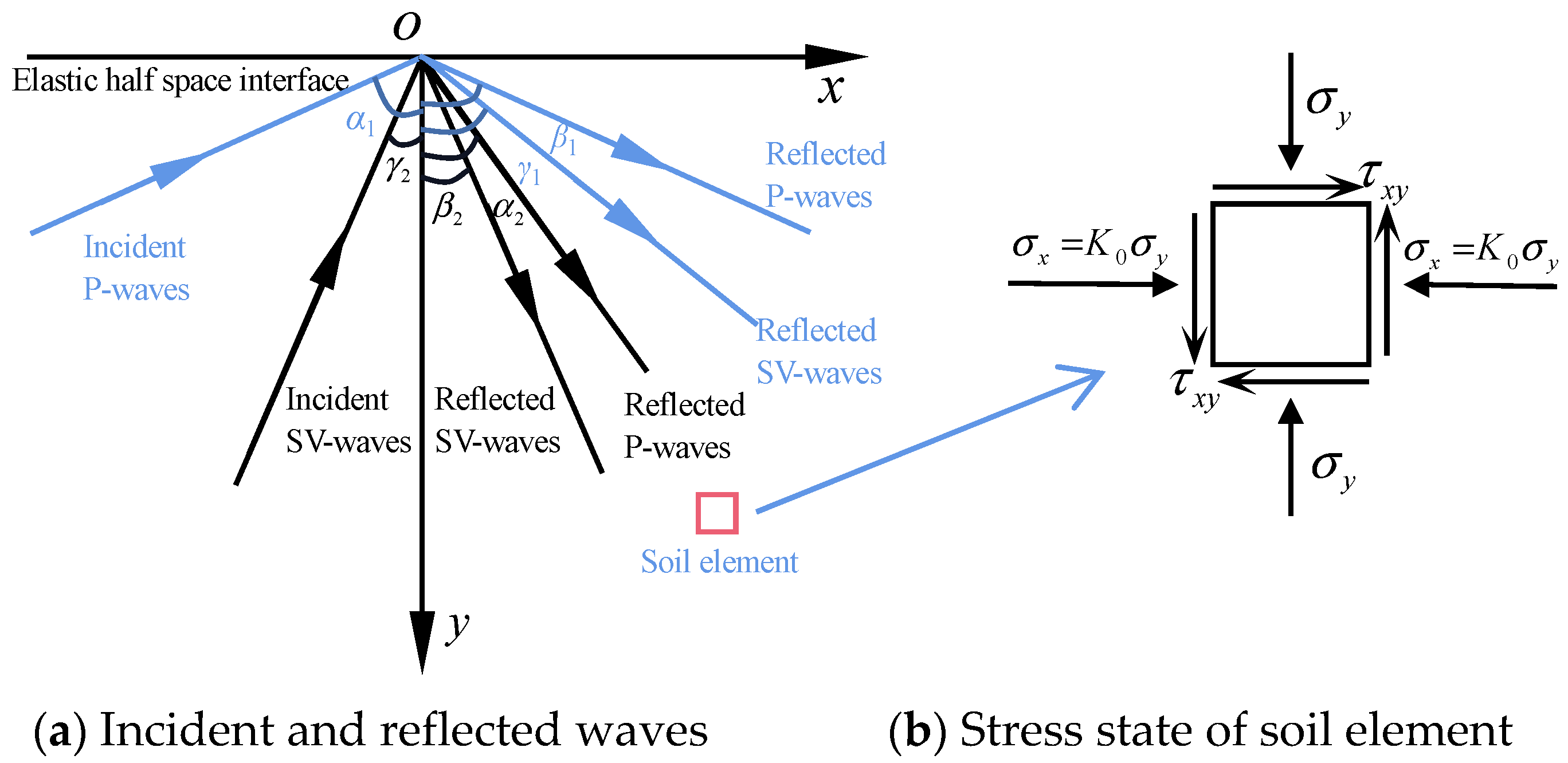
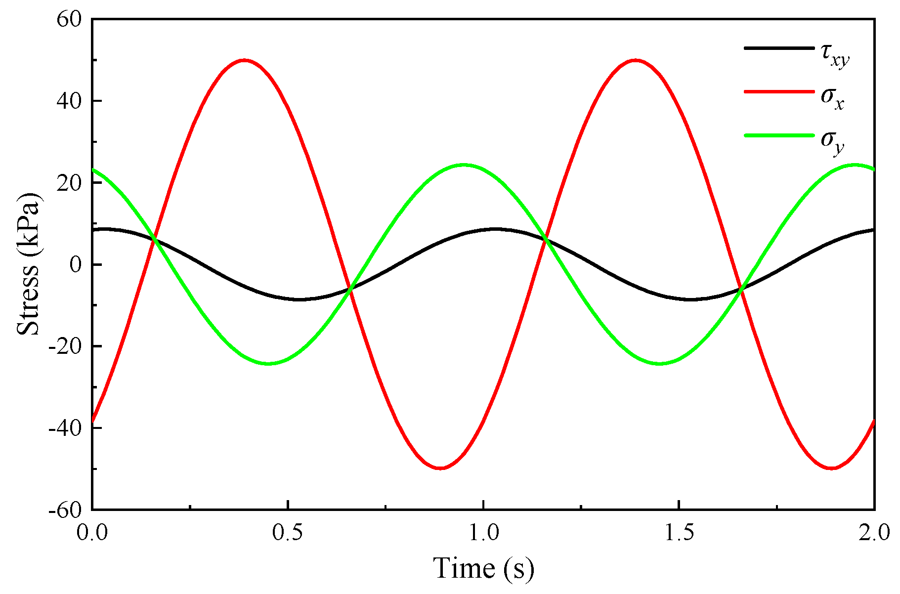
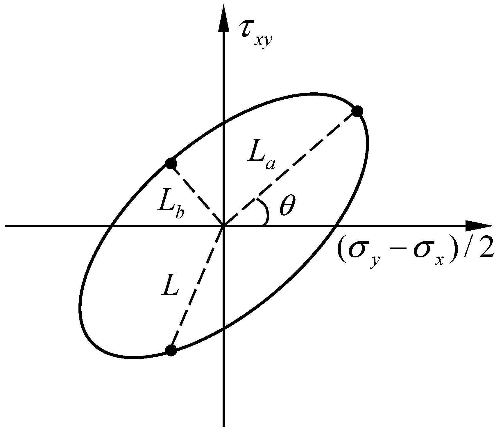
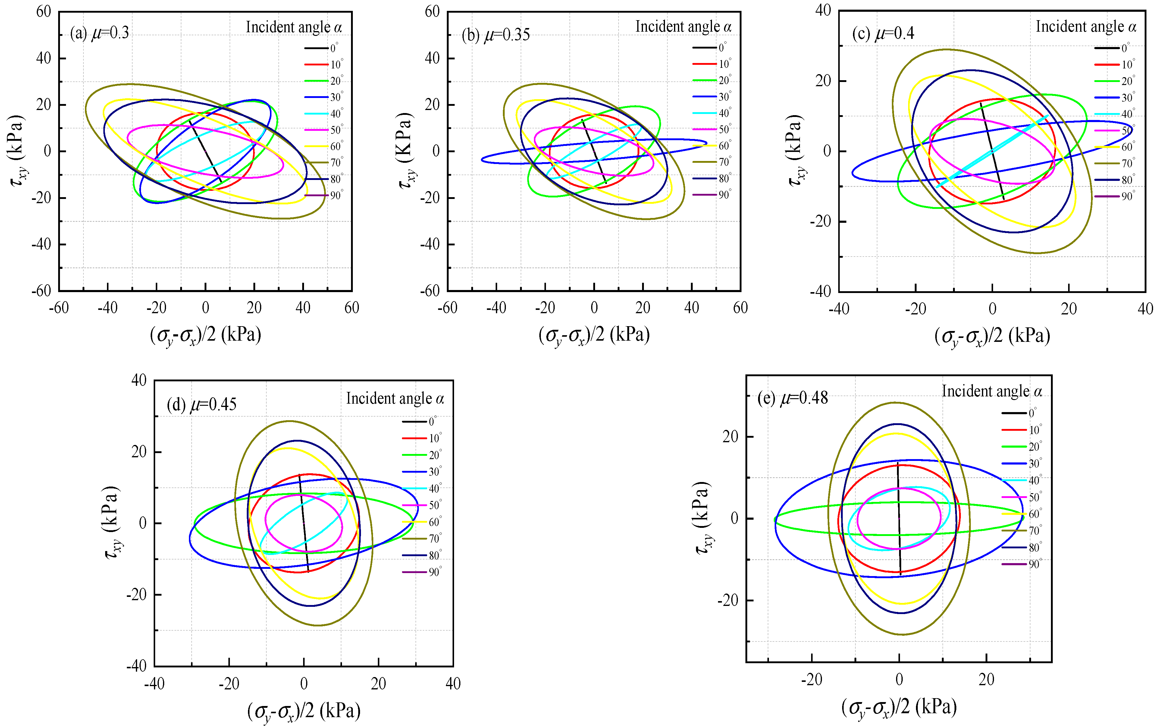
- This study derives the expression of dynamic stress components of soil element in the semi-infinite elastic space under obliquely incident P- and SV-waves, and obtains the corresponding dynamic stress path. It is found that the dynamic stress path of the soil element in − plane is usually an oblique ellipse.
- (2)
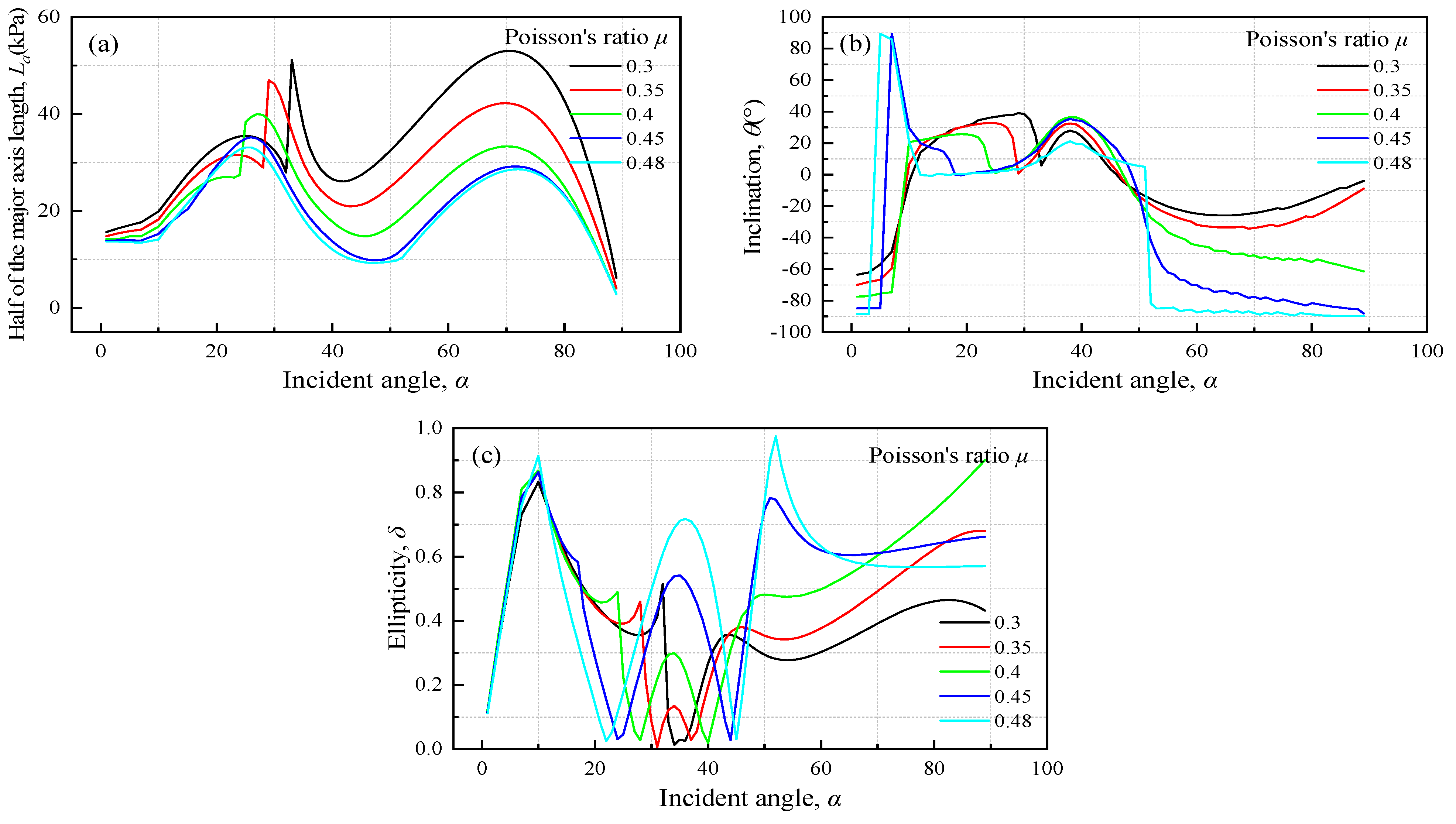
- The variation trend of La with the incidence angle exhibits double-peak curves for various Poisson’s ratio . La decreases gradually as increases. The maximum dynamic stress level for Poisson’s ratio of 0.3 is twice that for 0.48, the inclination angle of the elliptical stress path has an abrupt change when the soil is close to the full saturation. has a more significant impact on the inclination angle when ≥ 50°. The variation trend of with exhibits a triple-peak curve for different , and the peak value is greater for larger in the overall trend.
- (3)
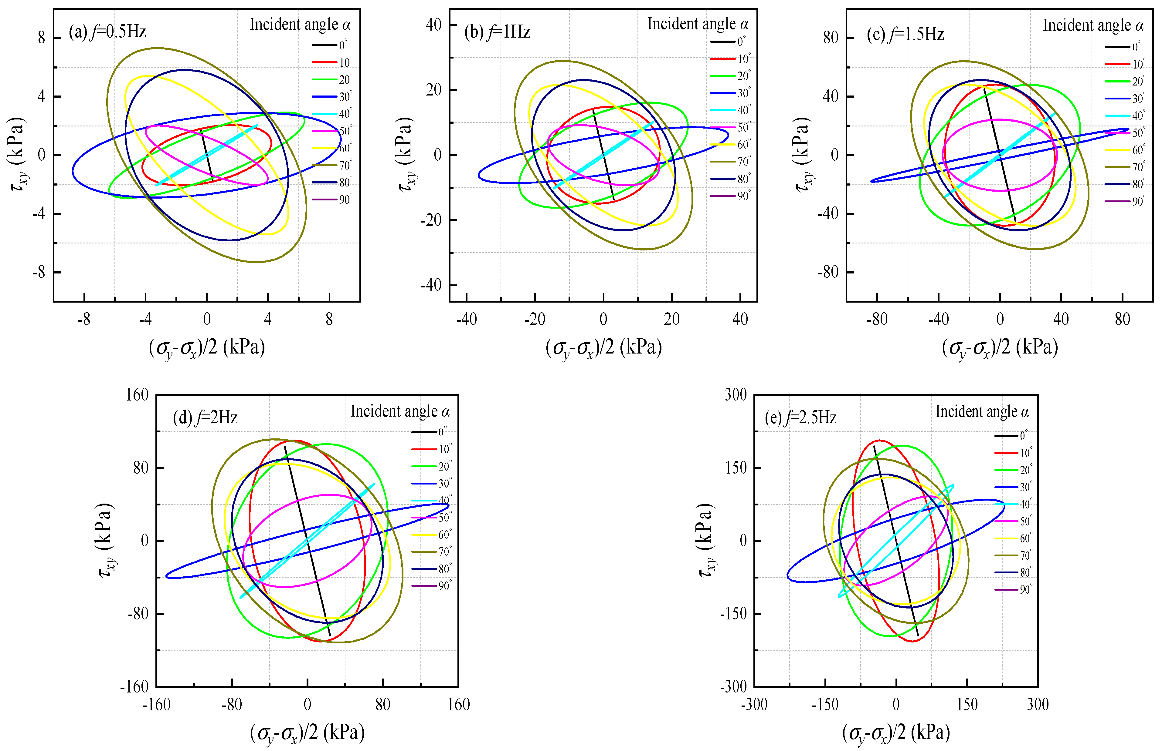
- La is greater for higher wave frequency at the same incident angle , which demonstrates that the dynamic stress level of soil element is greater with higher frequency. The dynamic stress level for 0.5 Hz approaches zero, and the maximum dynamic stress level for 2.5 Hz is about 6 times that for 1 Hz. When < 20°, increases significantly with , and the frequency has a significant impact on ; in this range of incidence angle, has an abrupt change from negative peak to positive peak. The variation trend of with exhibits triple-peak curves in the overall for various frequencies, and the frequency has a significant impact on .
- (4)
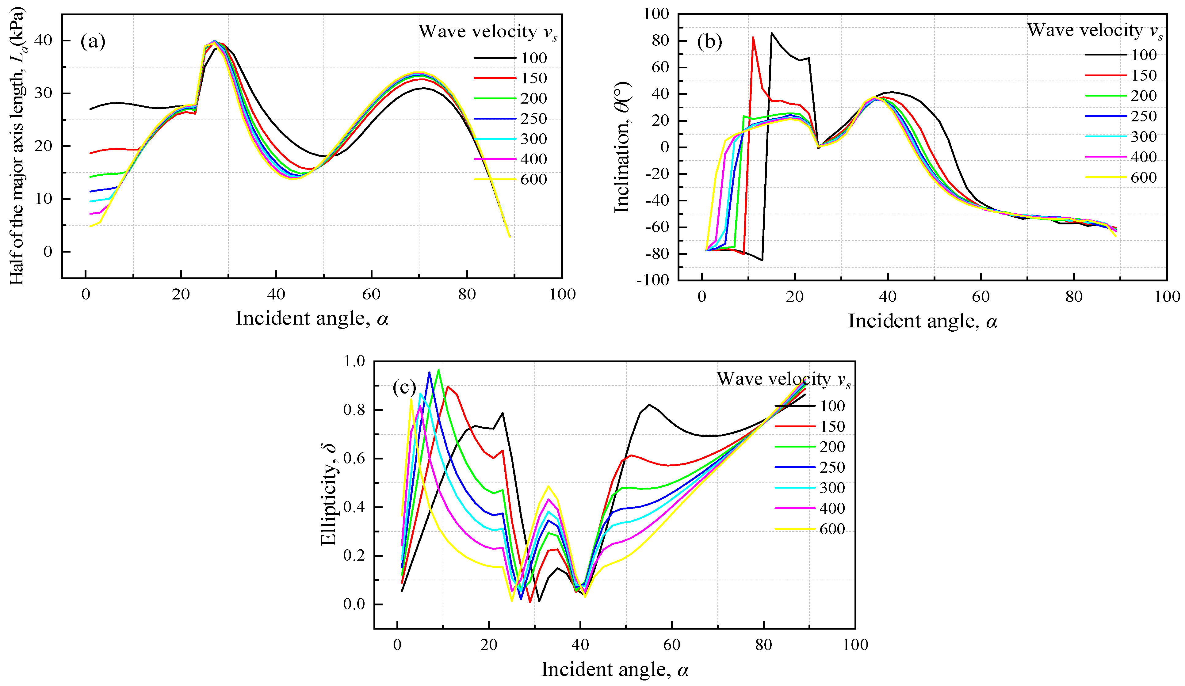
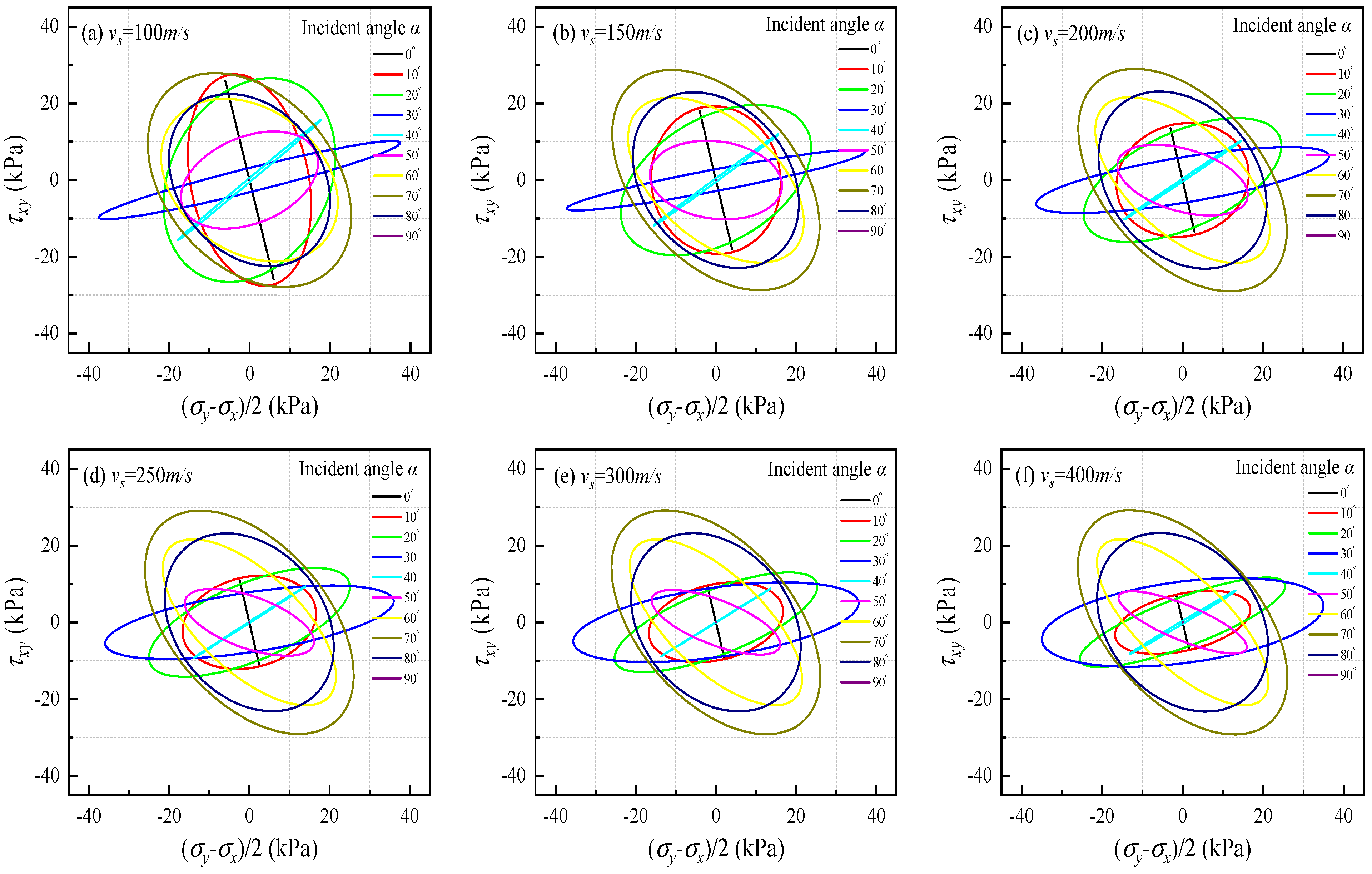
- The variation trend of La with exhibits double-peak curves in the overall for various wave velocities . Compared with the wave frequency, the influence of wave velocity on La is insignificant. The variation trend of with for various is similar to that for various frequency, and is larger for smaller . The variation trend of with exhibits triple-peak curves in the overall for various , and has a significant effect on . In general, the maximum dynamic stress level is about 40 kPa no matter how changes.
- (5)
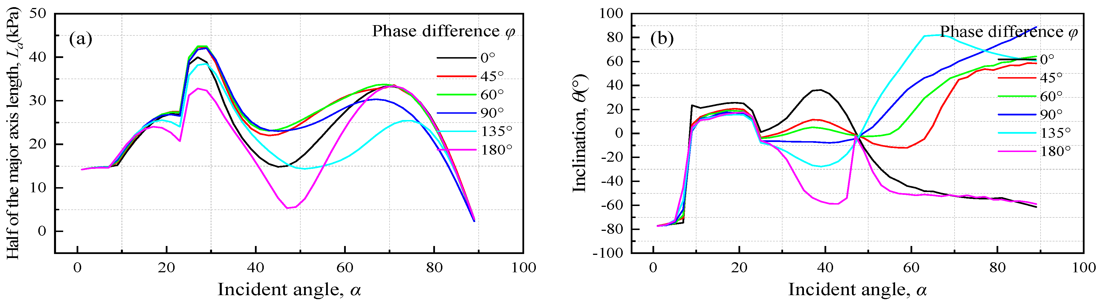
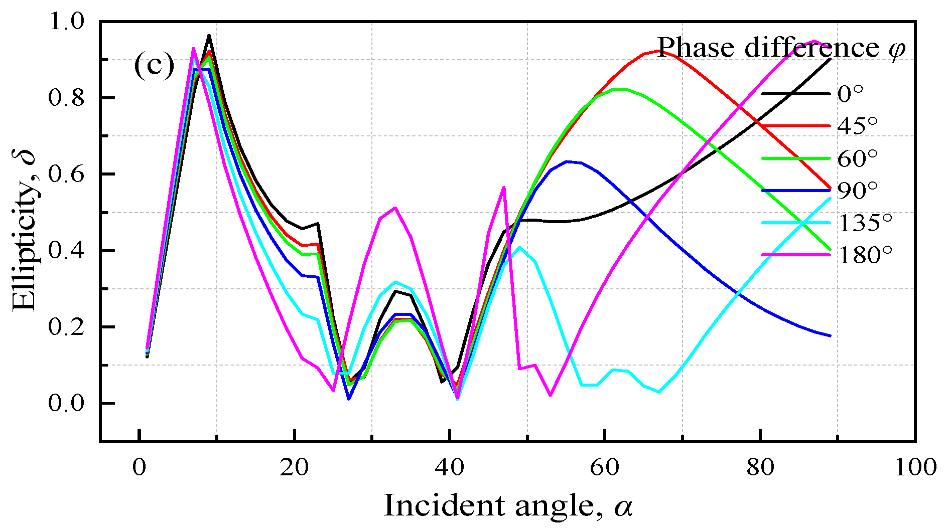
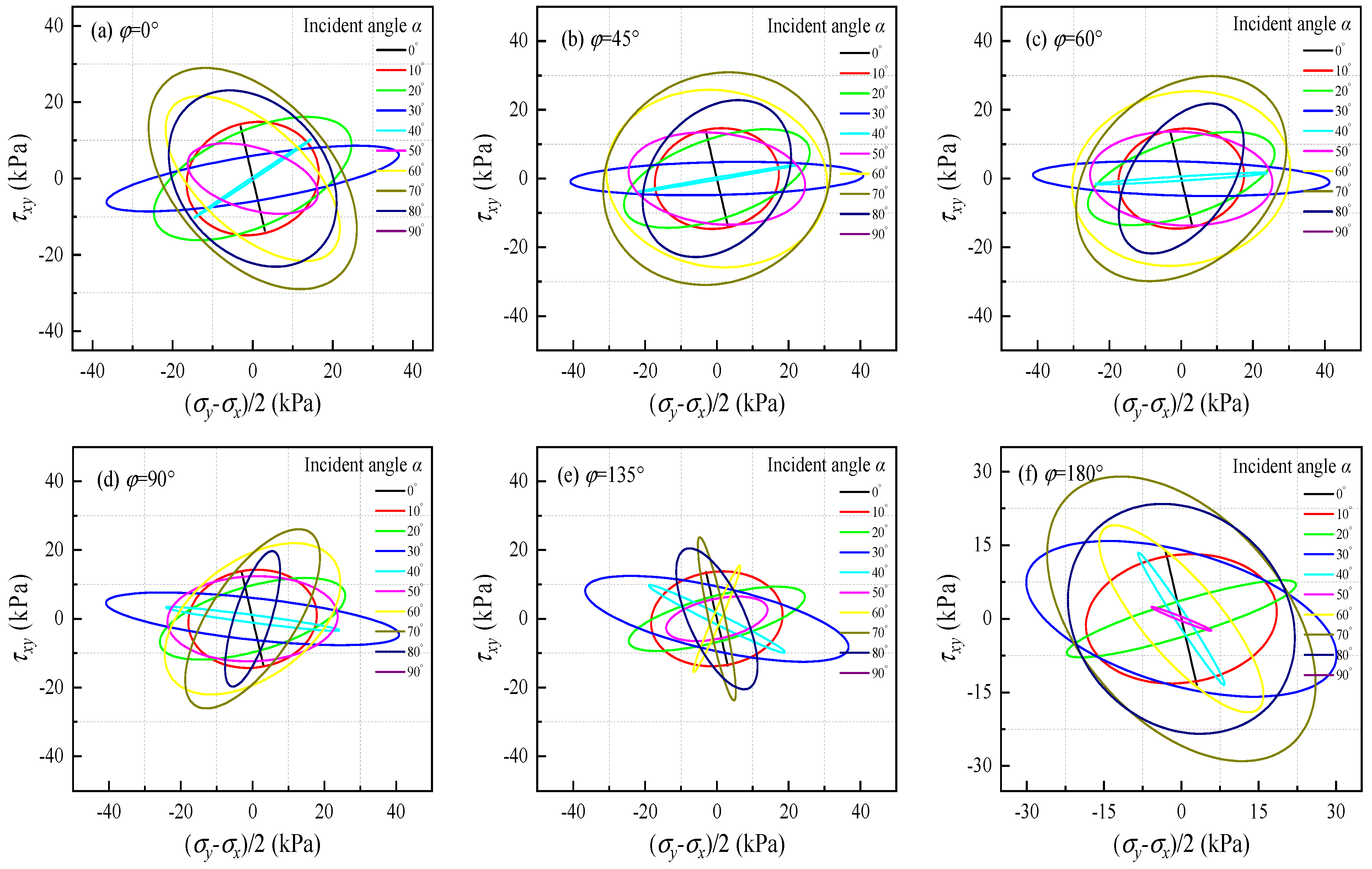
- The phase difference has less effect on La for approximate horizontal or vertical incidence, while it has greater effect on La under normal oblique incidence. The variation trend of with the incidence angle under different is quite different. reaches the second extreme value when is about 40°, and the extreme value is greater for smaller . The influence of on is insignificant when < 10°, but the influence is very significant when is within the range of 40–70°. In general, compared with other phase difference, the dynamic stress level for the phase difference of 60° is largest with a value of 43 kPa.
- (6)
- In the case of approximate vertical incidence, the elliptical stress path becomes more vertically slender as the soil depth increases, and the dynamic stress level of soil element gradually increases as the incident angle increases. The change in elliptical stress path becomes more complex in the case of oblique incidence. In the case of approximate horizontal incidence, the influence of soil depth on the elliptical stress path is insignificant, and the dynamic stress level of soil element decreases significantly as the incident angle increases. The dynamic stress level becomes greater as the soil depth increases, and the maximum dynamic stress level at 30 m depth is about 40 kPa.
Author Contributions
Funding
Data Availability Statement
Conflicts of Interest
Nomenclature
| Amplitude of incident P-wave | |
| Amplitude of reflected P-wave induced by incident P-wave | |
| Amplitude of incident SV-wave | |
| Amplitude of reflected SV-wave induced by incident SV-wave | |
| Amplitude of reflected SV-wave induced by incident P-wave | |
| Amplitude of reflected P-wave induced by incident SV-wave | |
| E | Elastic modulus |
| f | Wave frequency |
| G | Shear modulus |
| i | Complex number |
| k | Wave numbers |
| K0 | Coefficient of consolidation |
| L | Distance from any point on the elliptical stress path to the origin |
| La | Half of the major axis length |
| Lb | Half of the minor axis length |
| t | Time |
| u | Displacement components in x direction |
| vp | P-wave velocity |
| vs | Shear-wave velocity |
| vSV | SV-wave velocity |
| w | Displacement components in y direction |
| z | Soil depth |
| α | Incidence angle |
| α1 | Incident angle of P-wave |
| α2 | Reflection angle of P-wave induced by incident SV-wave |
| β1 | Reflection angle of P-wave induced by incident P-wave |
| β2 | Reflection angle of SV-wave induced by incident SV-wave |
| βcr | Critical incident angle |
| γ1 | Reflection angle of SV-wave induced by incident P-wave |
| γ2 | Incident angle of SV-wave |
| δ | Ellipticity |
| εx | Strain in x direction |
| εy | Strain in y direction |
| θ | Inclination angle |
| λ | Lame constant |
| μ | Poisson’s ratio |
| σy | Vertical stress (y direction) |
| σx | Horizontal stress (x direction) |
| ρ | Mass density of soil |
| τxy | Shear stress |
| Potential function for incident P-wave | |
| Potential function for reflected P-wave induced by incident P-wave | |
| Potential function for reflected P-wave induced by incident SV-wave | |
| Potential function for incident SV-wave | |
| Potential function for reflected SV-wave induced by incident P-wave | |
| Potential function for reflected SV-wave induced by incident SV-wave | |
| φ | Phase difference |
| ω | Circular frequencies |
References
- Seed, H.B.; Idriss, I.M. Simplified procedure for evaluating soil liquefaction potential. J. Soil Mech. Found. Div. Am. Soc. Civ. Eng. ASCE. 1971, 97, 1249–1273. [Google Scholar] [CrossRef]
- Seed, H.B.; Idriss, I.M.; Arango, I. Evaluation of liquefaction potential using field performance data. J. Geotech. Geoenviron. ASCE. 1983, 109, 458–482. [Google Scholar] [CrossRef]
- Jin, X.; Liao, Z.P. Statistical research on S-wave incident angle. Annu. Disas. Prev. Res. Inst. 1997, 40, 91–97. [Google Scholar]
- Wu, C.S.; Yu, T.T.; Peng, W.F.; Ye, Y.T.; Lin, S.S. Site response variation due to the existence of near-field cracks based on strong motion records in the Shi-Wen river valley, southern Taiwan. J. Geophys. Eng. 2014, 11, 055002. [Google Scholar] [CrossRef]
- Sigaki, T.; Kiyohara, K.; Sono, Y.; Kinosita, D.; Masao, T.; Tamura, R.; Yoshimura, C.; Ugata, T. Estimation of earthquake motion incident angle at rock site. In Proceedings of the 12th World Conference Earthquake Engineering, Upper Hutt, New Zealand, 30 January–4 February 2000. [Google Scholar]
- Zhao, R.B.; Bi, M.; Zhang, Y.; Liu, Z.X.; Wu, Z.Y. Half-space SV wave oblique incidence stress path in soil and hollow cylinder dynamic torsional shear test simulation. World Earthq. Eng. 2016, 32, 231–238. [Google Scholar]
- Huang, B.; Li, Q.Q.; Ling, D.S.; Wang, Y. Analysis of dynamic stress path due to oblique incidence of SV-waves and its influencing factors. J. Vib. Shock 2018, 37, 6–16. [Google Scholar]
- Hu, X.Q.; Wang, H.; Fu, H.T.; Liu, F.Y. Effects of bidirectional unconstant amplitude shear stress on dynamic properties of soft clay in under ellipse stress path. J. Southeast Univ. Engl. Ed. 2019, 49, 433–439. [Google Scholar]
- Du, X.L.; Huang, J.Q.; Zhao, M.; Jin, L. Effect of oblique incidence of SV waves on seismic response of portal sections of rock tunnels. J. Geotech. Eng. 2014, 36, 1400–1406. [Google Scholar]
- You, H.B.; Liang, J.W. Scattering of plane SV waves by a cavity in a layered half-space. Rock Soil Mech. 2006, 27, 383–388. [Google Scholar]
- Zhao, X.; Zhang, C.M.; Du, X.L.; Huang, J.Q.; Zhao, M. The analysis of the seismic response of mountain tunnels under SV waves with different incident directions. J. Vib. Eng. Technol. 2018, 31, 698–706. [Google Scholar]
- Wei, C.Q.; Yu, Y.Y.; Ding, H.P. Study on amplification characteristics of ground motion in layered basin in time and frequency domain under oblique incidence of SV wave. Earthq. Eng. Eng. Vib. 2022, 42, 225–234. [Google Scholar]
- Yin, C.; Li, W.H.; Zhao, C.G. Research of slope topographic amplification subjected to obliquely incident SV-waves. J. Vib. Acoust. 2020, 33, 971–984. [Google Scholar]
- Fu, F.; Zhao, C.G.; Li, W.H.; Zhang, W.H. Influence of local topographic on seismic response of tunnels subjected to obliquely incident SV waves. J. Beijing Jiaotong Univ. 2012, 36, 79–84. [Google Scholar]
- Roy, J.; Rollins, K.M.; Athanasopoulos-Zekkos, A.; Harper, M.; Linton, N.; Basham, M.; Zekkos, D. Gravel liquefaction assessment using dynamic cone penetration and shear wave velocity tests based on field performance from the 1964 Alaska earthquake. Soil Dyn. Earthq. Eng. 2022, 160, 107357. [Google Scholar] [CrossRef]
- Gičev, V.; Trifunac, M.D.; Orbović, N. Two-dimensional translation, rocking, and waves in a building during soil-structure interaction excited by a plane earthquake SV-wave pulse. Soil Dyn. 2016, 88, 76–91. [Google Scholar] [CrossRef] [Green Version]
- Huang, B.; Li, Q.Q.; Ling, D.S.; Liu, J.W.; Wang, Y. Analysis of the dynamic stress path under obliquely incident P-waves and its influencing factors. J. Zhejiang Univ. Sci. A 2017, 18, 776–792. [Google Scholar] [CrossRef]
- Cen, W.J.; Du, X.H.; Li, D.J.; Yuan, L.N. Oblique Incidence of Seismic Wave Reflecting Two Components of Design Ground Motion. Shock Vib. 2018. [Google Scholar] [CrossRef] [Green Version]
- Song, Z.Q.; Wang, F.; Li, Y.L.; Liu, Y.H. Nonlinear seismic responses of the powerhouse of a hydropower station under near-fault plane P-wave oblique incidence. Eng. Struct. 2019, 199, 109613. [Google Scholar] [CrossRef]
- Wang, D.G.; Shi, P.X.; Zhao, C.G. Two-dimensional in-plane seismic response of long-span bridges under oblique P-wave incidence. Bull. Earthq. Eng. 2019, 17, 5073–5099. [Google Scholar] [CrossRef]
- Liu, B.D.; Yu, M.; Wang, W.; Zhou, Z.H.; Li, X.J. Influence of Fault Parameters on Ground Motion under Incident P Waves. J. Earthq. Eng. 2017, 39, 160–167. [Google Scholar]
- Gao, X.J.; Qian, H.; Guo, Y.C.; Wang, F. Seismic response analysis of GRPS embankment under oblique incident P wave. J. Cent. South Univ. 2016, 23, 721–728. [Google Scholar] [CrossRef]
- Wang, M.H.; Chi, S.C. Dynamic response analysis of high earth-rockfill dam subjected to P wave with arbitrary incoming angles. Soil Dyn. Earthq. Eng. 2022, 157, 107260. [Google Scholar] [CrossRef]
- Naji, D.M.; Akin, M.K.; Cabalar, A.F. A comparative study on the VS30 and N30 based seismic site classification in Kahramanmaras, Turkey. Adv. Civ. Eng. 2020, 15, 8862827. [Google Scholar] [CrossRef]
- Skarlatoudis, A.A.; Thio, H.K.; Somerville, P.G. Estimating shallow shear-wave velocity profiles in Alaska using the initial portion of P waves from local earthquakes. Earthq. Spectra 2022, 38, 1076–1102. [Google Scholar] [CrossRef]
- Wu, Y.M.; Yen, H.Y.; Zhao, L.; Huang, B.S.; Liang, W.T. Magnitude determination using initial P waves: A single-station approach. Geophys. Res. Lett. 2006, 33, L05306. [Google Scholar] [CrossRef] [Green Version]
- Li, N.; Huang, B.; Ling, D.S.; Wang, Q.J. Experimental research on behaviors of saturated loose sand subjected to oblique ellipse stress path. Rock Soil Mech. 2015, 36, 156. [Google Scholar]
- Gu, C.; Cai, Y.Q.; Wang, J. Coupling effects of P-waves and S-waves based on cyclic triaxial tests with cyclic confining pressure. Chin. J. Geotech. Eng. 2012, 34, 1903–1909. [Google Scholar]
- You, H.B.; Zhao, F.X.; Rong, M.S. Nonlinear seismic response of horizontal layered site due to inclined wave. Chin. J. Geotech. Eng. 2009, 31, 234–240. [Google Scholar]
- Pan, D.G.; Lou, M.L.; Dong, C. Random wave-theory analysis of layered soil sites under P-wave and SV-wave excitation. J. Eng. Mech. 2006, 23, 66–71. [Google Scholar]
- Sawazaki, K.; Snieder, R. Time-lapse changes of P-and S-wave velocities and shear wave splitting in the first year after the 2011 Tohoku earthquake, Japan: Shallow subsurface. Geophys. J. Int. 2013, 193, 238–251. [Google Scholar] [CrossRef] [Green Version]
- Liu, Y.; Wu, R.S.; Ying, C.F. Scattering of elastic waves by an elastic or viscoelastic cylinder. Geophys. J. Int. 2000, 142, 439–460. [Google Scholar] [CrossRef] [Green Version]
- Farra, V.; Pšenčík, I. Moveout approximations for P-and SV-waves in VTI mediaMoveout approximations in VTI media. Geophysics 2013, 78, WC81–WC92. [Google Scholar] [CrossRef]
- Achenbach, J. Wave Propagation in Elastic Solids; Elsevier: Amsterdam, The Netherlands, 2012. [Google Scholar]
- Xu, Z.D. Seismic Wave Theory; Tongji University Press: Shanghai, China, 1997. [Google Scholar]
- Niu, B.H.; Sun, C.Y. Half Space Medium and Seismic Wave Propagation; Petroleum Industry Press: Beijing, China, 2002. [Google Scholar]
- Wu, S.M. Soil Dynamics; China Architecture and Building Press: Beijing, China, 2000. [Google Scholar]
- Kumari, P.; Sharma, V.K.; Modi, C. Reflection/refraction pattern of quasi-(P/SV) waves in dissimilar monoclinic media separated with finite isotropic layer. J. Vib. Control. 2016, 22, 2745–2758. [Google Scholar] [CrossRef]
- Chattopadhyay, A.; Venkateswarlu, R.L.K.; Saha, S. Reflection of quasi-P and quasi-SV waves at the free and rigid boundaries of a fibre-reinforced medium. Sadhana 2002, 27, 613–630. [Google Scholar] [CrossRef] [Green Version]
- Yoshimi, Y.; Tanaka, K.; Tokimatsu, K. Liquefaction resistance of a partially saturated sand. Soils Found. 1989, 29, 157–162. [Google Scholar] [CrossRef] [PubMed]
- Yang, J. Reappraisal of vertical motion effects on soil liquefaction. Geotechnique 2004, 54, 671–676. [Google Scholar] [CrossRef]
- Yang, J.; Sato, T. Interpretation of seismic vertical amplification observed at an array site. Bull. Seismol. Soc. Am. 2000, 90, 275–285. [Google Scholar] [CrossRef]
- Ishihara, K.; Towhata, l. Sand response to cyclic rotation of principal stress directions as induced by wave loads. Soils Found. 1983, 23, 11–26. [Google Scholar] [CrossRef] [Green Version]
- Allen, R.M.; Kanamori, H. The potential for earthquake early warning in southern California. Science 2003, 300, 786–789. [Google Scholar] [CrossRef] [Green Version]
- Liu, H.; Zheng, T.; Bo, J. Statistical analysis of uncertainty for shear wave velocities of cohesive soils. World Inf. Earthq. Eng. 2010, 26, 99–103. [Google Scholar]
- Miao, Y.; He, H.; Liu, H. Reproducing ground response using in-situ soil dynamic parameters. Earthq. Eng. Struct. Dyn. 2022, 51, 2449–2465. [Google Scholar] [CrossRef]
- Wang, S.Y.; Zhuang, H.Y.; Zhang, H. Near-surface softening and healing in eastern Honshu associated with the 2011 magnitude-9 Tohoku-Oki Earthquake. Nat. Commun. 2021, 12, 1–10. [Google Scholar]


Publisher’s Note: MDPI stays neutral with regard to jurisdictional claims in published maps and institutional affiliations. |
© 2022 by the authors. Licensee MDPI, Basel, Switzerland. This article is an open access article distributed under the terms and conditions of the Creative Commons Attribution (CC BY) license (https://creativecommons.org/licenses/by/4.0/).
Share and Cite
Wang, M.; Song, L.; Cheng, X.; Zhang, J.; Lu, L.; Li, W. Dynamic Stress Path under Obliquely Incident P- and SV-Waves. Buildings 2022, 12, 2210. https://doi.org/10.3390/buildings12122210
Wang M, Song L, Cheng X, Zhang J, Lu L, Li W. Dynamic Stress Path under Obliquely Incident P- and SV-Waves. Buildings. 2022; 12(12):2210. https://doi.org/10.3390/buildings12122210
Chicago/Turabian StyleWang, Mingyuan, Linfeng Song, Xinglei Cheng, Jianxin Zhang, Liqiang Lu, and Wenqian Li. 2022. "Dynamic Stress Path under Obliquely Incident P- and SV-Waves" Buildings 12, no. 12: 2210. https://doi.org/10.3390/buildings12122210