Article

Magnetic Signal Characteristics in Critical Yield State of Steel Box Girder Based on Metal Magnetic Memory Inspection

Department of Civil Engineering, Xi’an University of Architecture and Technology, Xi’an 710055, China
*
Author to whom correspondence should be addressed.
Buildings 2022, 12(11), 1835; https://doi.org/10.3390/buildings12111835
Submission received: 23 September 2022 / Revised: 20 October 2022 / Accepted: 21 October 2022 / Published: 1 November 2022
(This article belongs to the Section Building Structures)

Abstract

:
Metal magnetic memory testing (MMMT) is a nondestructive testing technique that can detect early signs of damage in components. Many scholars have studied the effect of uniaxial stress on the self-magnetic-leakage field (SMLF)’s strength. Nevertheless, there is still insufficient research on the combined action of bending and shear. We studied the law of distribution of the magnetic signal,   Δ H SF ( y ) , at different stress parts of a steel box girder and the quantitative relationship between the magnetic characteristic parameters and the external load. The results showed that the MMMT could accurately detect the early stress concentration zone (SCZ) and predict the final buckling zone of steel box girders. It could be judged that the corresponding parts of the steel box girder had entered the elastic-plastic working stage by the reverse change of the   Δ H SF ( y ) -F and   | H SF ( y ) | a   -F curve trends, this feature could be used as an early warning sign before the steel box girder was deformed or destroyed. The fitted   | H SF ( y ) | a v e   -F linear expression could be used as the expression between the magnetic signal and the shear capacity. All the evaluation methods were expected to provide a basis for effectively evaluating the stress state of steel box girders with the MMMT method.

1. Introduction

Steel box girders are widely used in bridge structures because of their lightweight, high strength, good plasticity, significant flexural stiffness, and strong torsional resistance, and they are suitable for various complex systems [1,2]. Owing to material inhomogeneity and various microscopic defects, a local stress concentration zone (SCZ) often appears in steel box girders under a working load. When the SCZ reaches the yield load, the components will create a local buckling phenomenon, and the structural damage caused by the buckling instability of the components will have a serious impact on the safety of human life and property. There have been many accidents caused by buckling instability in history. Li [3] reported that during the construction of the Westgate bridge near Melbourne, the top flange plate at the midspan lost stability after buckling, leading to the collapse of the entire span of 112 m. The former Soviet Union counted 59 major steel structure accidents during 27 years, of which 29% were the overall lost stability or local lost stability of the structure. In the 1970s, in less than two years, four orthotropic deck slab bridges under construction in Europe suffered from collapse after local buckling. In recent years, there have been many accidents caused by a bridge’s local buckling. Because the steel box girder is prone to local buckling, many scholars [4,5,6,7] have studied how to improve the local stiffness and strength and how to enhance the local stability of the steel box girder.
Aiming at the instability phenomenon of the bridge steel structure after local buckling, if the location of the local stress concentration and critical yield state of the steel structure could be identified and an early warning provided through the results of nondestructive testing (NDT), the potential safety risks could be found in time and disasters could be avoided. Therefore, early identification of the stress concentration location and the critical yield state of steel structures in service by the NDT method is an important basis for evaluating structure reliability [8]. However, it is difficult for traditional NDT to effectively evaluate such invisible hidden damage [9,10].
Metal magnetic memory testing (MMMT) is a new NDT method proposed by Dubov, and its essence lies in the magnetomechanical effect. Under the combined action of the geomagnetic field and external stress, the irreversible movement and reorientation of the domain wall will cause a change in the self-magnetic-leakage fields (SMLF) in defects and in the SCZ. Thus, the sudden change in the SMLF on the component surface characterizes its local stress and damage [11,12]. Compared with traditional NDTs, MMMT does not require cleaning the surface of the specimen or applying a couplant, and it does not require a strong external magnetic field either; therefore, it is simple to operate and has a low cost. Most importantly, MMMT can not only detect formed macrodamage, but also predict the location of the damage, and offer early diagnosis of ferromagnetic components based on the comprehensive analysis of the location of the maximum stress concentration and the damage source.
Based on the unique advantages of the MMMT, scholars studied its feasibility in identifying the location of SCZ and evaluating the degree of stress concentration of ferromagnetic components, and, gradually, it has been applied in the field of damage inspection of engineering structures. In terms of the MMMT diagnosis of SCZ, the magnetic dipole model theory believed that the defect or SCZ could be accurately located through zero-crossing of the normal magnetic signal and the extreme value of the tangential magnetic signal. Zhang et al. [13] showed that the magnetic signal had extreme value at the defect location of the steel plate, so it could be judged that the defects and residual stresses inside the steel plate at the extreme of the magnetic signal were more serious than those in other locations. Roskosz et al. [14,15] studied the relationship between the magnetic signal distribution and the stress distribution of ferromagnetic materials in static tensile tests. The results showed that the correlation between the magnetic signal gradient and the stress was better than that between the magnetic signal and the stress on the specimen surface. In terms of MMMT evaluating the degree of stress concentration, Dong et al. [16] found that the magnetic field gradient K increased with the stress concentration factor increasing, which could be used to characterize the degree of stress concentration on the surface of ferromagnetic materials. Huang et al. [17] considered that the ratio of the maximum value of the normal magnetic signal gradient Kmax to the average magnetic signal gradient value Kstd could be used to quantitatively describe the degree of stress concentration. Bao et al. [18] proposed a new damage evaluation parameter—magnetic concentration factor am—to describe the degree of stress concentration. In the application of MMMT, Dubov et al. took the lead in applying the MMMT to the on-site inspection of hot water boilers [19]. At present, this technology has been applied to engineering fields such as oil and gas pipelines [20,21], gears [22], welded steel structures [23], crane rails [24], railways [25], etc.
Currently, MMMT is still an emerging NDT method. Previous experimental studies mainly focused on the uniaxial tension or compression of steel plates, and the conclusions were only applicable to the case of macroscopic defects in specimens. However, the problems related to invisible hidden damage in steel components, such as inspection of local buckling location, identification, and warning of the critical yield state were not been considered. To further study the feasibility of MMMT for invisible hidden damage monitoring of complex steel structures, and also to extend the application of MMMT to bridge steel structures, a four-point bending static loading test was carried out on the steel box girder in this paper. We analyzed the feasibility of identifying the location of invisible hidden damage on different parts of the steel box girder through magnetic signal characteristics. Then, two magnetic parameters were proposed to be used as warning signs of critical yield state on different parts of the steel box girder. Finally, the relationship between the magnetic signal value and the magnetic parameters was obtained to inverse the force state of the web.

2. Experiments

2.1. Material Properties

Q345qC steel is widely used in welded components of bridge steel structures on account of its good mechanical properties, welding properties, and low-temperature deformation ability. Thus, the bending test of the Q345qC steel specimen based on MMMT has important theoretical and engineering value. In the test, the C, Si, Mn, P, and S content of the Q345qC steel was 0.18%, 0.06%, 0.4%, 1.2%, and 0.002%, respectively. According to the Chinese standard (GB/T228.1–2010), tensile tests were carried out on three standard plates at room temperature to determine the mechanical properties of the materials, and the test results were taken as the average of the three specimens. The results showed that the elastic modulus, yield strength, tensile strength, and elongation of the Q345qC steel were 201 GPa, 424 MPa, 564 MPa, and 29%, respectively.

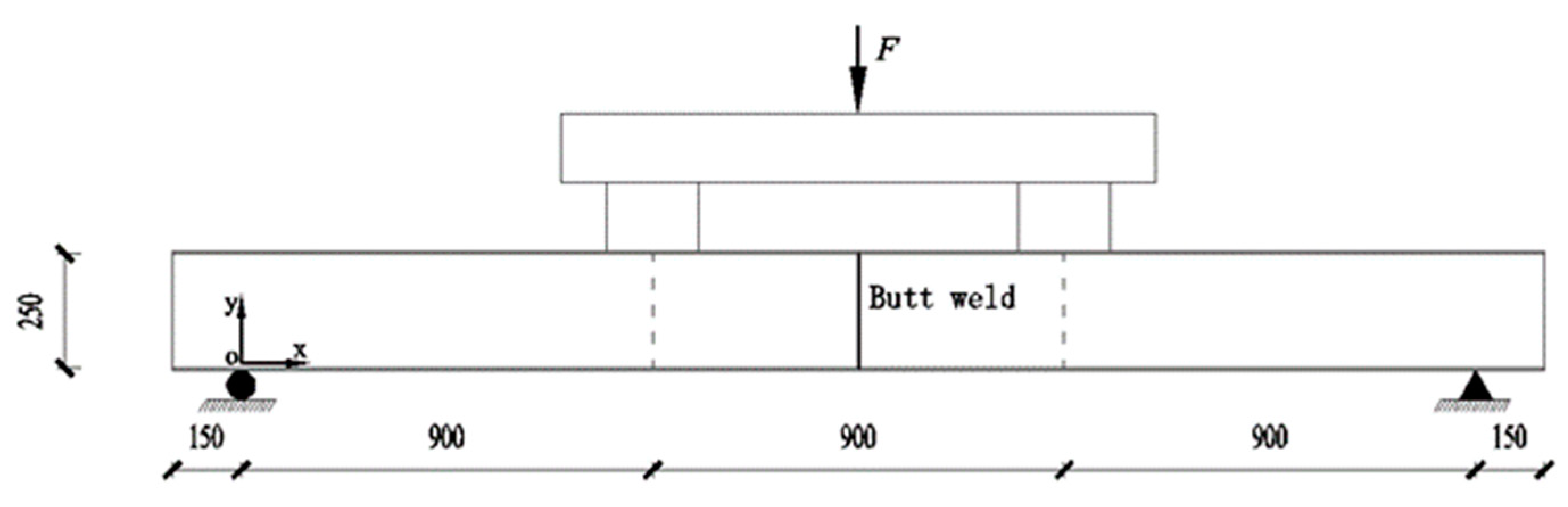
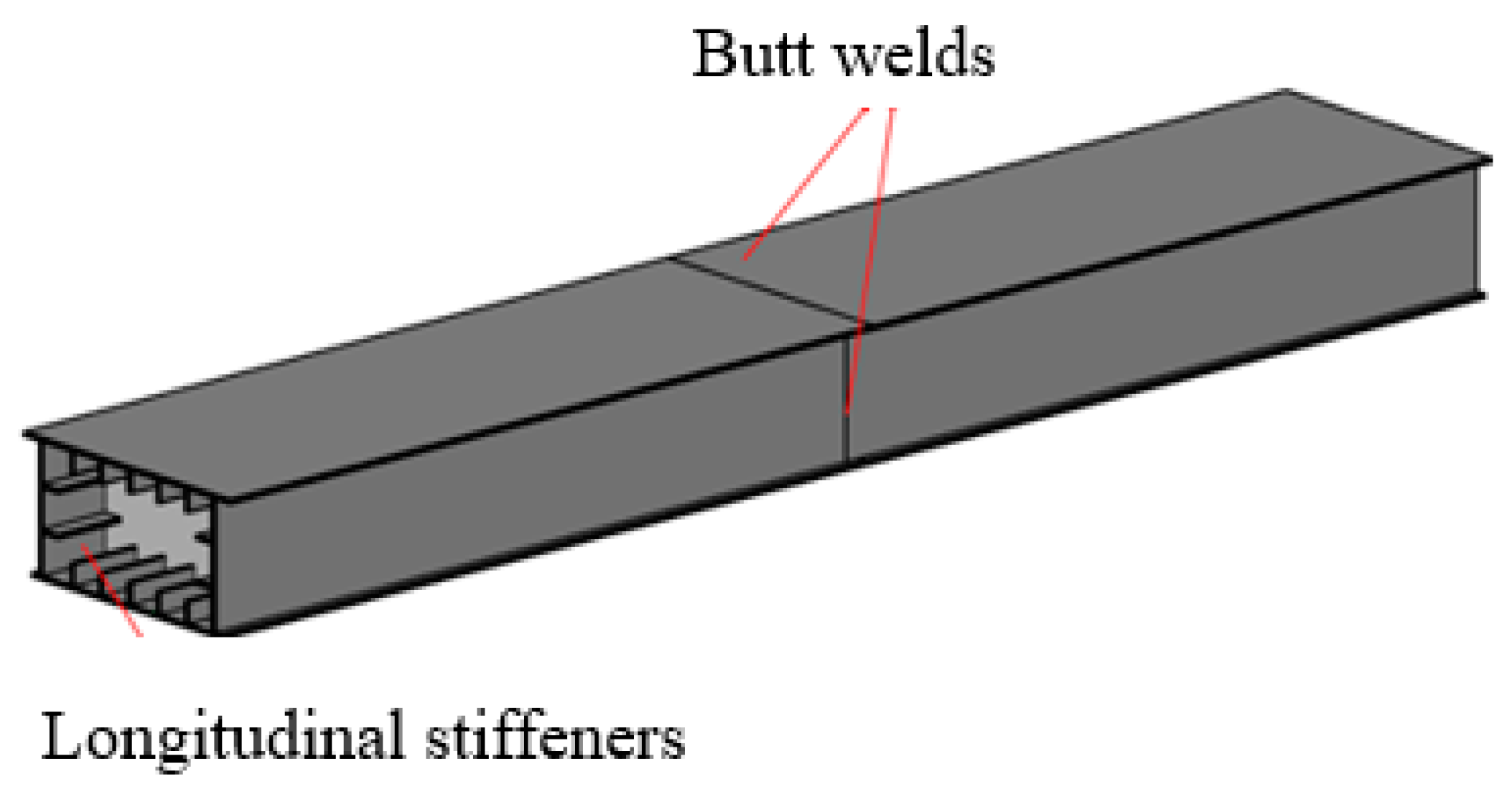
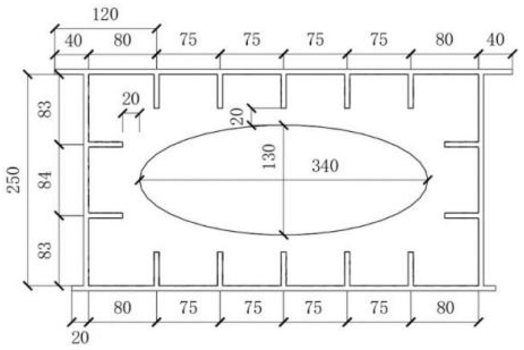
2.2. Specimen Details

Figure 1 shows the schematic diagram of the four-point bending load of the specimen. For the specimen, the length was 3000 mm, the width of the top and bottom flanges was 540 mm and 500 mm, respectively, the webs were perpendicular to the flanges, and the height was 250 mm. An amount of 150 mm was reserved outside the supports on both sides so that the effective length of the specimen was 2700 mm. Five longitudinal stiffeners were evenly arranged on the top and bottom flanges, and three on both sides of the webs, and the height of the stiffeners was 40 mm. The thickness of the Q345qC steel was 6 mm. From the support, 10 diaphragms were evenly arranged along the length of the beam with a spacing of 300 mm, which were closely bonded with the top and bottom flanges and the webs on both sides. The butt welds were arranged at X-1350 mm of the web and X-1380 mm of the top and bottom flanges. Figure 2 and Figure 3 show the 3D model diagram and the cross-sectional dimension of the specimen, respectively.

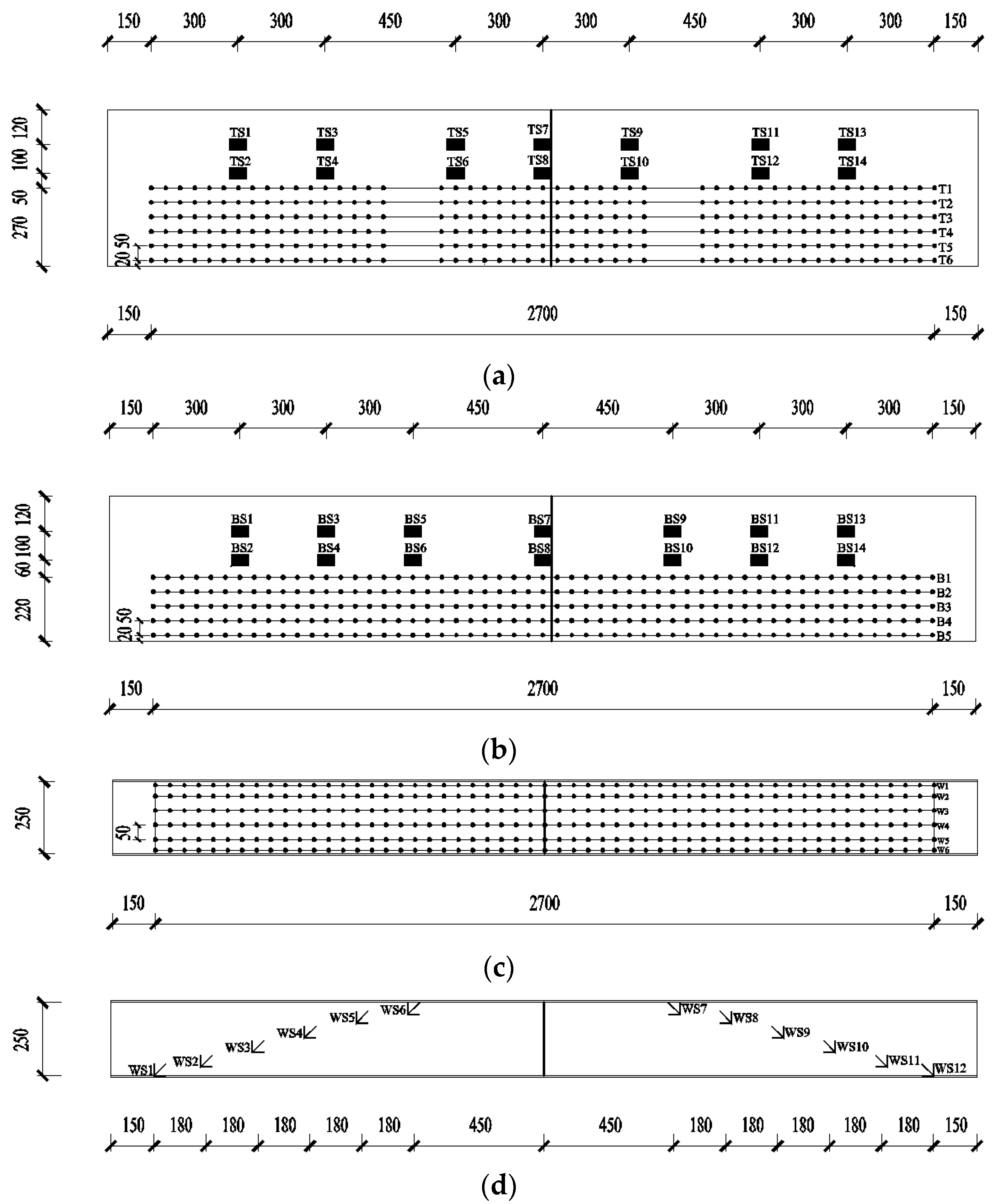
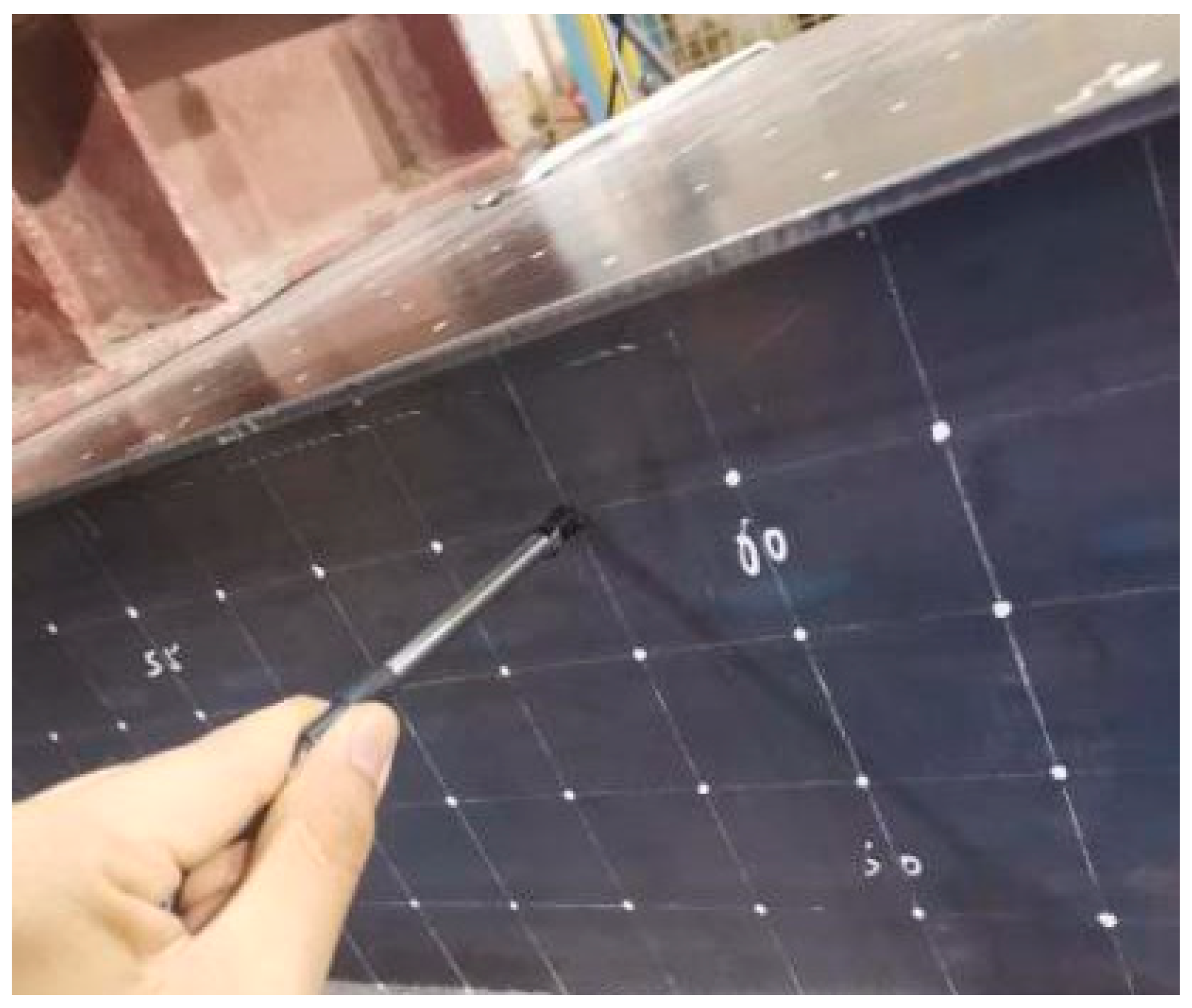
2.3. Layout Plan of Inspection Points

Six inspection lines were arranged on the top flange surface and marked T1–T6. Five inspection lines were arranged on the bottom flange surface and marked B1–B5. Six inspection lines were evenly set on the web and marked W1–W6. The spacing between all inspection lines was 50 mm, and the inspection points spaced at 50 mm intervals were evenly arranged along the direction of the inspection line. Significantly, the inspection points were encrypted at the loading end and around the butt welds. Because the encryption points did not affect the law of the magnetic signal, the data of the encryption points were not analyzed in this paper.
Fourteen strain gauges were arranged on the top and bottom flanges and marked TS1–TS14 and BS1–BS14, respectively. On the web, six 45°-strain rosettes were evenly arranged on the inclined line from the supports on both sides to the loading end and marked WS1–WS12. It was worth noting that to reduce the interference of the strain gauges on the magnetic signal value, strain gauges were arranged on one side of the specimen and inspection points were arranged symmetrically on the other side. The schematic diagram of the inspection points and strain gauges is shown in Figure 4.

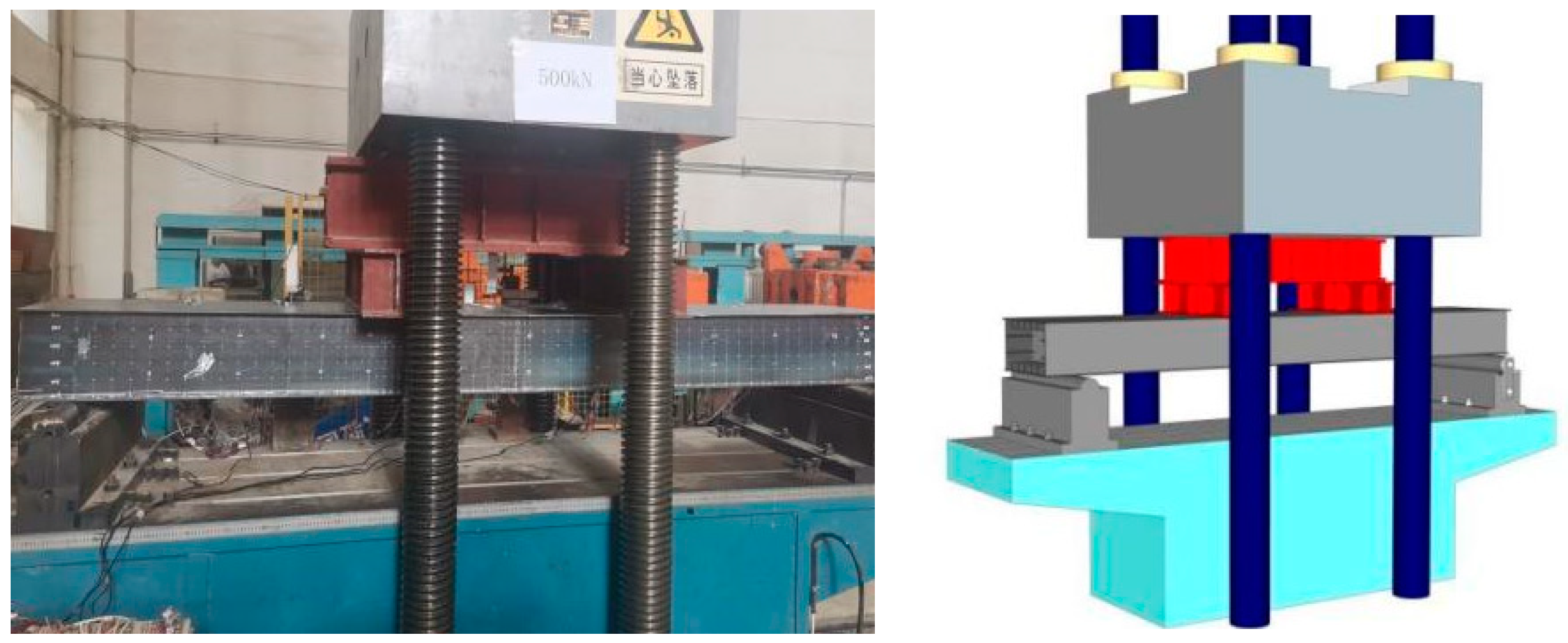
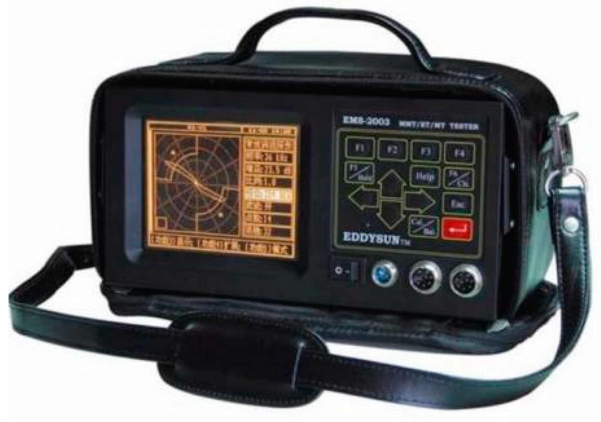
2.4. Experimental Instruments and Test Setup

The test was conducted using a YAW-5000 electrohydraulic servo loading instrument, and Figure 5 shows the test device and schematic diagram. The concentrated load was converted into a region load and applied to the specimen through a distribution beam having a width of 200 mm. The actual loading levels in the test were 150, 300, 400, 500, 570, 650, 725, 800, 850, 925, 1000, 1100, 1117 kN, and the failure load. Figure 6 shows the load-displacement curve in the midspan of the specimen. The results showed that the specimen undergoes elastic, elastoplastic, and plastic deformations as the load increases. The specimen yielded at about 565 kN, and then, reached the ultimate load at about 1117 kN.
The specimen was placed on the loading platform in the north–south direction, and the initial magnetic signal of each inspection line on the surface was measured. When the specimen loaded to the preset value, the magnetic signal was measured in the same way as detecting the initial state. Magnetic signals were collected by the EMS-2003 intelligent metal magnetic memory detector (Figure 7). The instrument was equipped with a hall pen probe with a measuring range of ±1000 Am−1 and a sensitivity of 1 Am−1. We normalized the probe before each inspection to reduce the interference of the environmental magnetic field on the magnetic signal. During the test, the magnetic signal inspection direction was from left to right, the probe was vertically placed on the surface of the specimen (Figure 8), and the constant lift-off value was maintained. Three magnetic signals were collected at each measuring point, and the average value was calculated to reduce the effect of random errors. After that, the specimen was further loaded to a higher preset value and the above steps were repeated until the specimen was damaged. Additionally, researchers usually demagnetize specimens before testing and offline measure SMLF intensity [8]. However, the steel box girder bears a working load with no demagnetization condition in practical engineering. In this study, the normal component of the SMLF on the surface of the steel box girder, namely, the magnetic signal H SF ( y ) , was measured under maintained loading.

3. Test Results and Analysis

The V-groove butt weld in the middle span of the specimen was welded using E50 electrodes and the strength and stiffness of the weld were slightly higher than that of the steel. Due to the impact of the butt weld, the buckling deformation that should have occurred in the midspan location of the top flange was shifted, and the final buckling area occurred between 1550 and 1650 mm. Among them, the number represents the distance from the left support to a certain inspection point, and the buckling deformation photo is shown in Figure 9. The buckling area occurred on the steel, and the welded joint was not in a weak position, so the weld did not weaken the load-bearing capacity of the specimen. Relevant studies showed that high-quality welds had some influence on the location of the buckling deformation, and generally had little impact on improving load-bearing capacity [26,27].
Due to the space limitation, one inspection line was selected on the top flange, bottom flange, and web, namely, T2, B1, and W3 for analysis. For the flanges, the stress on the pure bending section was much greater than the bending shear section, and for the web, the bending shear section on both sides was much greater than the pure bending section. Therefore, this paper focused on analyzing the pure bending section of the flanges and the bending shear sections of the web.

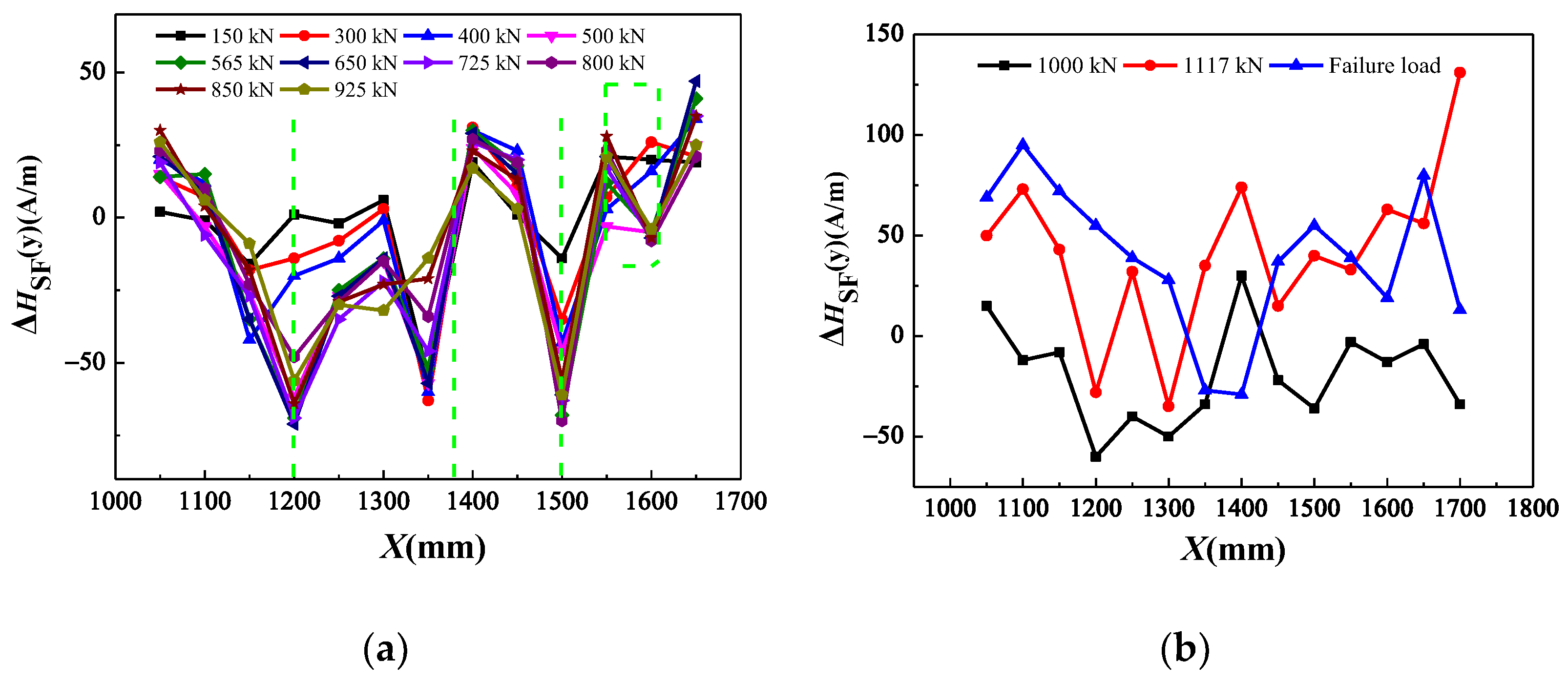
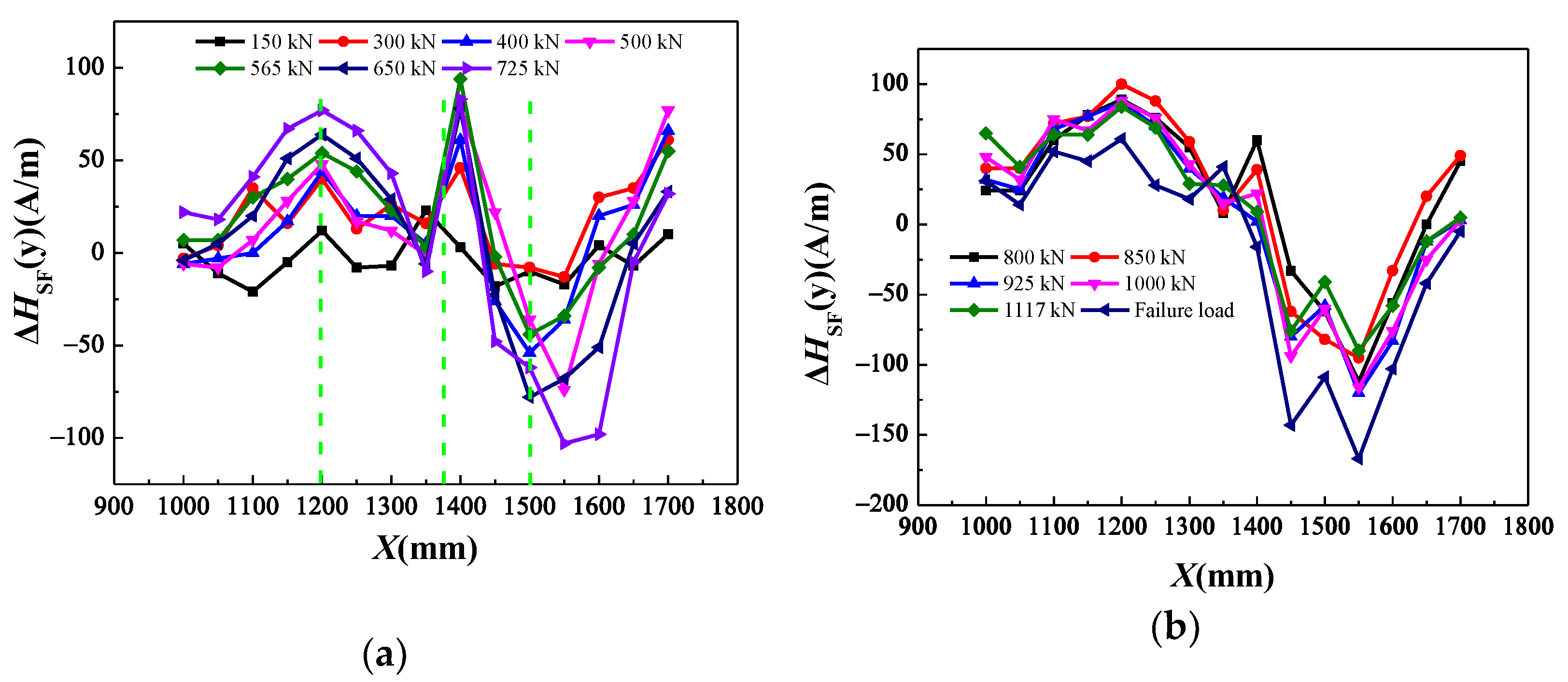
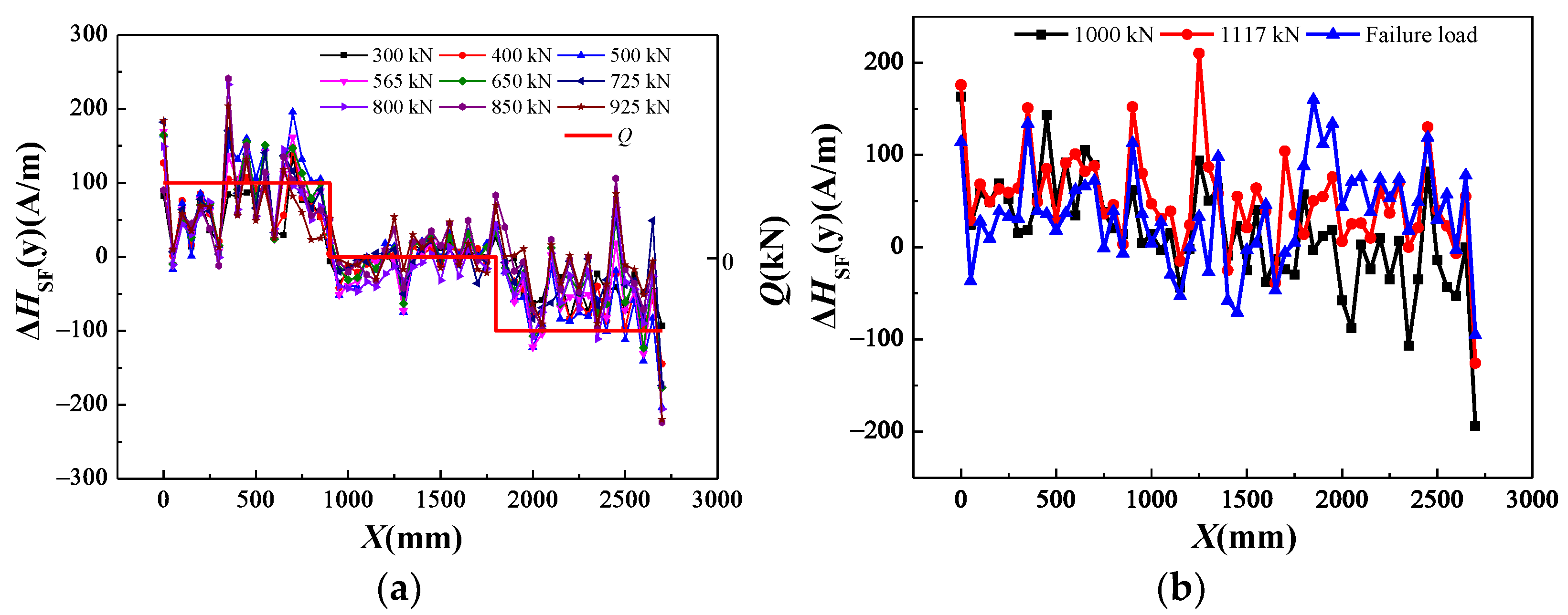
3.1. Distribution Law of Magnetic Signal

At the zero-load stage, due to various internal friction effects, different degrees of magnetization appear in a specimen, and impurities or defects in the manufacturing process cause a decrease in local permeability, thus forming a high magnetoresistance region, which hinders the passage of magnetic force lines. An uneven magnetic potential difference is formed in defect areas, which distorts the originally uniform magnetic force lines, thereby generating an unequal SMLF. This affected the judgment of the signal feature points on the surface of the specimen during the loading process. Gorkunov [28] reported that different remanence states significantly affect the stability of inspection results with the MMMT method. Therefore, in this paper, the initial residual magnetic field value was subtracted from the measured value of each inspection point and marked as   Δ H SF ( y ) . Figure 10, Figure 11 and Figure 12 show the   Δ H SF ( y )   curves at the flanges of the specimen. In the figures, the blue dotted line and the dotted box represent the SCZ and buckling failure position, respectively.
As shown in Figure 10a, in the elastic and elastoplastic loading stages, the   Δ H SF ( y ) curves gradually tended to be consistent under different loads, especially after 400 kN. This is due to the piezomagnetic effect. The magnetic domain rotates along the tensile stress or perpendicular to the compressive stress direction after applying load to mild steel [29], and the magnetization of the material also changes. The locations of 1200 mm and 1500 mm were the SCZs caused by diaphragms, where the curves just had an extreme value under different loads. External stress accelerated the movement of the magnetic domain wall and the rotation of the magnetic moment, resulting in a significant increase in the magnetic field strength in the SCZ. The location of 1380 mm was the SCZ caused by the butt weld, and the curves on both sides of the butt weld exist as the minimum and maximum values. The reason is that the welding joint is composed of the steel notch and welding material, and the magnetic permeability of the steel is different from welding materials. The magnetic field line penetrates from steel into welding material and then from welding material into steel, and the material parameters undergo two sudden changes, resulting in two sudden changes in the magnetic field strength. This theory is also applicable to the formed defects, such as cracks and notches. There were multiple extreme values on the curve between 1550 and 1650 mm, which presaged this region existed as a SCZ, while Figure 9 shows that this region happens to be in the buckling position. In engineering, this discriminant method can be used to detect the location of early SCZs and predict the damage location. From Figure 10b, the magnetization behavior in the plastic stage was relatively complex, and extremum characteristics of the   Δ H SF ( y )   curves at the SCZs disappeared.
Figure 11 shows that the magnetic characteristics of the SCZ on the bottom flange were similar to those of the top flange. For the bottom flange of the tension zone, the range of   Δ H SF ( y )   in the elastic loading stage was −103–94 A/m, whereas in the top flange of the compression zone it was −70–53 A/m and the values were significantly reduced. This is in line with the basic theory of the MMMT method, that is, the magnetization under tensile stress is different from that under compressive stress, and   Δ H SF ( y )   is more sensitive to tensile stress.
It is noteworthy that the classic method for MMMT to detect SCZs is that the normal magnetic signal of the SCZ is zero value, and the peak and trough are on both sides of the stress concentration area [8,19]. Many scholars have verified the theory by conducting uniaxial stress tests on demagnetized specimens. Chen [30] reported that for a nondemagnetized plate under uniaxial stress, the initial residual magnetic field value was subtracted from the measured value of each inspection point and zero-crossing the point of the new curve was the SCZ. However, Su [31] reported that the normal magnetic field intensity was not necessarily zero in the SCZ during the online test. Guo [32] reported that when the portal frame was inspected online, the magnetic signal at the stress concentration zones appeared as an extreme value. Zhang [13] reported that the magnetic signal curve had extreme points where the defects existed. The steel box girder also obtained a similar phenomenon as above.
From Figure 12, the web was mainly subjected to shear force, resulting in less stress on the diaphragm and butt weld during the loading process, and the magnetic signal characteristics on it were not obvious. Significantly, the   Δ H SF ( y ) curves were clearly divided into three segments in the elastic and elastoplastic loading stages. On the pure bending section, due to the small shear force value, the   Δ H SF ( y ) curves were approximately a horizontal line fluctuating around zero and the   Δ H SF ( y ) value on the left bending shear section was greater than zero, and on the right was less than zero. The   Δ H SF ( y ) curves were consistent with the distribution law of the shear force on the web, which showed that the magnetic field can be used to characterize the stress state of the steel box girder, and the change of the magnetic signal changes correspondingly with the change in the stress state. In the plastic deformation stage, the curves’ fluctuation increased, and the characteristic of the curves disappeared.

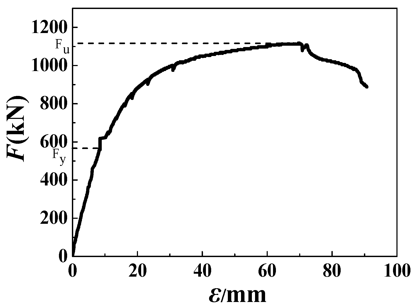
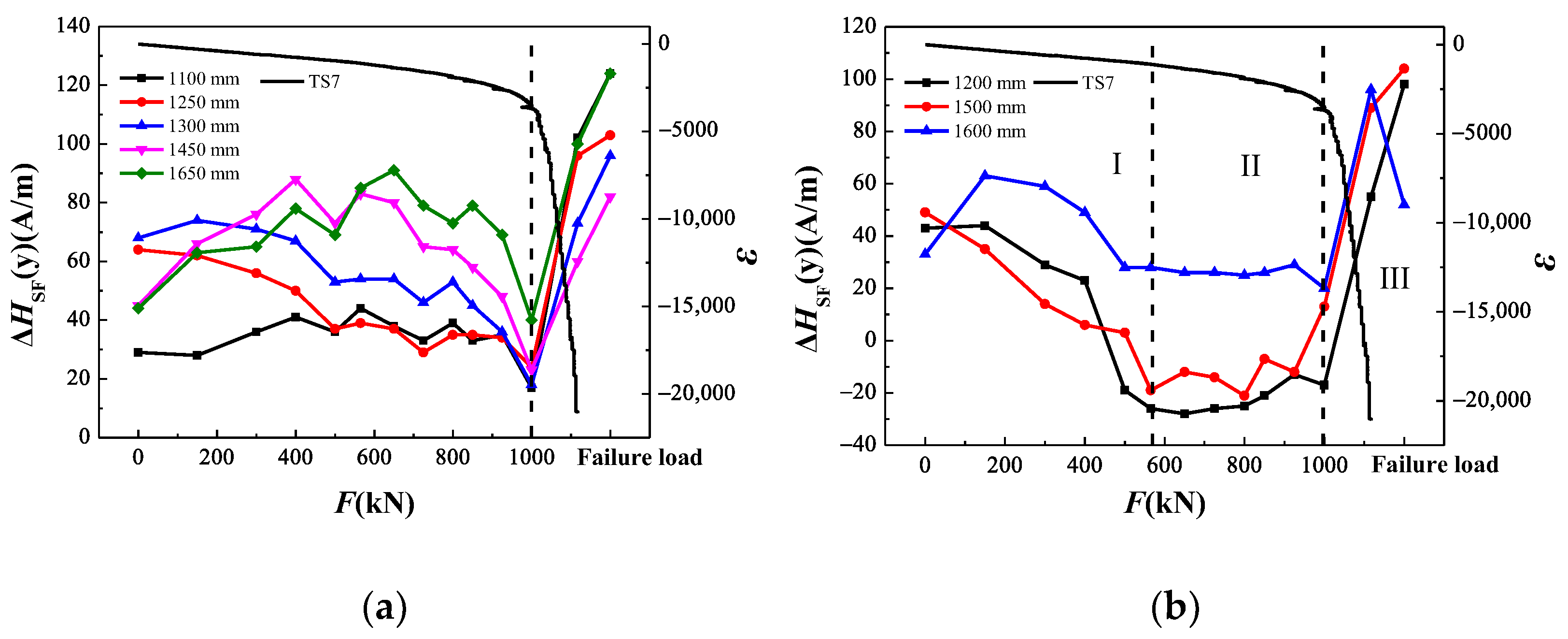
3.2. Force Magnetic Relationship

The biggest advantage of the MMMT method is that it can detect SCZs without evident defects to realize the early diagnosis of ferromagnetic components. With the change of external load, the SMLF strength of the specimen surface also changes. Through the changing characteristics of the magnetic signal it can qualitatively judge the critical characteristics of the stressed components in the elastic and elastoplastic, elastoplastic and plastic working stages, and an early warning can be given before the box girder is deformed or destroyed.
The   Δ H SF ( y ) -F and ε-F curves of the top and bottom flanges and the web are shown in Figure 13, Figure 14 and Figure 15, respectively. From the strain data, the maximum strain of the top and bottom flanges was at the midspan and was marked TS7 and BS7, respectively. At 540 and 2160 mm of the web, the strain in the 45° direction of the strain rosette was the largest and was marked WS4 and WS9.
As seen in Figure 13a, the curve trends were similar for each inspection point. When loaded to 1000 kN, each curve converged and appeared with a unique extreme value. From the strain curve, the load corresponding to this extreme value was exactly the critical load in the elastoplastic and plastic deformation stages. With the further increased load, the curves suddenly changed in a reverse direction, and the top flange entered the plastic failure stage. Su [33] carried out a four-point bending test on a corrugated-web steel box girder without diaphragms. The test results in the figure are almost the same as those at the same position in Su’s test, which proves the reliability of the test results. In engineering, the sudden and rapid reverse change of the trend of the Δ H SF ( y ) -F curve can be used to diagnose whether the top flange is in the plastic deformation stage. As seen in Figure 13b, the curves on the SCZ were obviously different from that of others. The curves could be divided into three parts: Ⅰ, Ⅱ, and Ⅲ according to the curve characteristics, which corresponded to the completely elastic stage, elastoplastic stage, and plastic deformation stage, respectively. Through this feature, the stress state of the top flange could be diagnosed. In the elastic loading stage, that is, before 565 kN, the   Δ H SF ( y ) changed approximately linearly with the load increasing. In the elastic–plastic stage, that is, between 565–1000 kN,   Δ H SF ( y )   had little change. In the plastic deformation stage, that is, after 1000 KN,   Δ H SF ( y )   changed rapidly in reverse. In engineering, whether in the SCZ or at other locations, the sudden and rapid reverse change of the trend of the   Δ H SF ( y ) -F curve can be used to diagnose whether the top flange is in the plastic deformation stage.
From Figure 14, in the elastic and elastoplastic loading stages, each curve gradually rose with the load increasing, and when loaded to 850 kN, the curves showed a maximum value. According to the strain curve, at this time, the bottom flange entered the plastic deformation stage, and then, the curves decreased rapidly with the load increasing. In engineering, the sudden and rapid reverse change of the trend of the   Δ H SF ( y ) -F curve can be used to diagnose whether the bottom flange is in the plastic deformation stage. The bottom flange was mainly subject to tensile stress, and the test phenomenon in the figure was consistent with that under uniaxial tensile stress. Due to the top and bottom flanges mainly bearing compressive and tensile stress, respectively, the changing trend of the   Δ H SF ( y ) -F curve of the two was the opposite. Therefore, the changing trend of the curve can be used to judge whether a part of the specimen was under pressure or tension. This result was similar to the test result of Yi et al. [34]. In addition, unlike the top flange, the SCZ (1200 mm) on the bottom flange was not significantly different from other areas. This may be because the top flange directly bore the load from the loading end. The maximum stress and failure area appeared on the top flange. The stress concentration degree of the SCZ in the top flange was much larger than that of the bottom flange, resulting in the unique magnetic characteristics of the top flange.
Because the bending shear sections on both sides of the web mainly bore shear stress, the strain values of each inspection point were different. In this paper, only the inspection points close to WS4 and WS9 were analyzed. As seen in Figure 15, under the action of shear stress, the absolute value of the   Δ H SF ( y )   increased first and then decreased with load increase. When loaded to 565 kN, the curves showed an extreme value. At this load, the slope of the load–strain curve began to change, which indicated that this load could be considered as the yield load. In engineering, the sudden and rapid reversal of the   Δ H SF ( y ) -F curve trend can be used to detect whether the web has yielded. This discrimination method plays a role in early warning of web damage.

3.3. Discussion of the Laws of Magnetic Signals

The top and bottom flanges and web mainly bore compressive stress, tensile stress, and shear stress, respectively. Previous studies showed that the magnetization mechanism under uniaxial compressive stress was very complex, and the top flange of the steel box girder was even more complex. Because the   Δ H SF ( y ) distribution laws of bottom flange and web were similar, only the web was discussed below.

3.3.1. Elastic Loading Stage

Jiles and Sablik et al. [35,36] argued that the physical essence of the force–magnetic effect lies in the equivalence of the stress action and the magnetic field action. The external stress changes the magnetostrictive coefficient, resulting in the change of the effective field; that is, the external stress is equivalent to adding an equivalent magnetic field Hσ in the ferromagnet. The system energy A along the reversible nonhysteresis magnetization curve is as shown in [37]:
A = μ 0 H M + μ 0 2 α M 2 + 3 2 σ λ + T S
where μ 0 = 4 π × 10 7   H · m 1 is the vacuum permeability, H is the applied magnetic field, M is the magnetization, α is the coupling coefficient of the internal magnetic domain, σ is the stress, λ is the magnetostriction coefficient, T is the temperature, and S is the entropy.
The first-order differential of A to M is the effective field He of the ferromagnetic component under the combined action of external stress and magnetic field, as follows:
H e = 1 μ 0 d A d M = H + a M + 3 2 σ μ 0 ( d λ d M ) σ
when the stress inside the material is not coaxial with the magnetization, for isotropic polycrystalline ferromagnetic materials, He can be expressed as follows:
H e = H + a M + H σ = H + a M + 3 2 σ μ 0 ( d λ d M ) σ ( cos 2 θ v sin 2 θ )
where v is the Poisson’s ratio. In this test, the specimen was placed in the north–south direction, and its web was subjected to shear stress. The stress directions were approximately perpendicular to the direction of the geomagnetic field, ignoring the deflection angle of the geomagnetic field, and θ was assumed to be 90°.
λ was determined as a function of M and σ, and expanded using the Taylor series, by omitting higher-order terms, as follows [38]:
λ = [ γ 1 ( 0 ) + γ 1 ( 0 ) σ ] M 2
where γ 1 ( 0 ) = 7 × 10 18   m 2   · A 2 and γ 1 ( 0 ) = 1 × 10 25   m 2   · A 2   [39].
The magnetization, M, can be expressed by the Langevin function as follows [39]:
M = M s [ cot h ( H e u 0 a ) μ 0 a H e ]
where Ms is the saturation magnetization.
Expanding the series of hyperbolic cosine function as follows:
cot h   x = 1 x + x 3 x 3 45 + 2 x 5 945
when |x| < 1, omitting the higher-order term in Equation (6), the magnetization, M, could be simplified as follows:
M = M s H e 3 μ 0 a
Substituting Equations (4) and (7) into (3), and equating γ = γ 1 ( 0 ) + γ 1 ( 0 ) σ , the following was obtained:
H e = 3 μ 0 a H 3 μ 0 2 a M s a μ 0 + 3 M s v γ σ
Taking the partial derivative of the He with respect to the stress σ, as follows:
H e σ = 9 μ 0 a H M s v ( 7 × 10 18 1 × 10 25 σ ) ( 3 μ 0 2 a M s a μ 0 + 3 M s v γ σ ) 2
Let, H e / σ   = 0, then σ = 35 MPa. When σ > 35 MPa, then H e / σ > 0. In this stage, the effective magnetic field strength increased with increasing stress. The effective field strength is proportional to the magnetization, and the magnetization is proportional to the magnetic field strength; therefore, the magnetic field strength   H SF ( y ) measured on the material surface was proportional to the effective field strength. The steel type in this test was Q345qC, and the yield strength was 424 MPa. Therefore, the   Δ H SF ( y )   measured in the elastic loading stage increased gradually with the load increasing. The above was the reason why the amplitude of the magnetic signal increased in the elastic stage.

3.3.2. Plastic Deformation Stage

The magnetization behavior of ferromagnetic materials in the plastic stage is relatively complex. Plastic deformation led to a large increase in dislocation density and then led to dislocation entanglement, which hindered the movement of magnetic domain walls in the form of pinning points [8]. As the plastic deformation increases, the dislocation density increases, and the pinning of the domain wall becomes stronger. Su [23] reported that for crystal materials, the reciprocal of initial permeability μ i   and coercive force   H C was proportional to the square root   Λ   of the dislocation density, that is, 1 / μ i ~ H C Λ . As the dislocation density Λ   increased, the initial permeability μ i   decreased and the coercivity   H C   increased. As the permeability decreased, the magnetization also decreased, and at the same time, the material was harder to magnetize due to the increased coercivity. These were the reasons for the decreased of magnetic signal amplitude in the plastic stage.

4. Analysis of Magnetic Characteristic Parameters

4.1. Damage Warning Analysis Based on the Magnetic Characteristic Parameter

The   Δ H SF ( y ) value of a single inspection point may result in measurement errors. If a statistical method was used, the measurement error would have been smaller, and the test results would have been easier to analyze. The stress on all the inspection points in the pure bending section of the flange was almost equal, and the same was true on a certain inspection line in the bending shear section of the web. Moreover, the sign of the magnetic signal only represented the direction of the magnetic field strength and not the magnitude. Therefore, the mean value of the absolute value of the magnetic signal,   | H SF ( y ) | a , was defined to characterize the force–magnetic relationship, and the expression is as follows:
| H SF ( y ) | a = [ | H SF ( y ) i | ] / N
where   H SF ( y ) i   is the magnetic signal value of a measuring point. N is the number of measuring points on the corresponding inspection line. Figure 16 shows the   | H SF ( y ) | a   curves at the top flange, bottom flange, and web of the specimen, where T and TS were the numbers of the inspection line and strain gauge on the top flange, respectively. Similarly, B and BS, W and WS were on the bottom flange and web, respectively. The specific locations of inspection lines and strain gauges at different force parts correspond to Figure 4a–d, respectively.
As seen in Figure 16a, in the elastic loading stage,   | H SF ( y ) | a gradually increased with the load increasing. When loaded to 650 or 725 kN, the curves showed an extreme value. From the strain curve, the load was approximately the yield load, which represented the limit of the structure’s safe state. In the elastic-plastic stage, about 650–1000 kN,   | H SF ( y ) | a decreased first and then increased with the load increasing. In the plastic deformation stage, that is, after 1000 kN,   | H SF ( y ) | a increased rapidly. When loaded to the ultimate load of 1117 kN,   | H SF ( y ) | a reached the maximum value, which meant the specimen was about to fail. In view of the phenomenon that   | H SF ( y ) | a increased again after the top flange yielded, some scholars reported that after the compression member entered the elastoplastic stage, a large plastic flow occurred inside it, the original lattice structure was damaged, and a new lattice structure was formed. At this time, the gap cracks at the measuring point were compressed, the structure was more uniform and denser, the deflection of the magnetic domain was further developed, and the magnetic signal was further increased [40].
As seen in Figure 16b,c, unlike the top flange, the   | H SF ( y ) | a on the bottom flange and web first increased and then decreased with the load increasing. The difference in curve distribution trend was caused by different kinds of forces. The load corresponding to the peak value on the curves of the bottom flange was 725–850 kN. At this time, the bottom flange was approximately in the elastoplastic working stage. The load corresponding to the peak on the curves of the web was 565 kN, which was approximately the yield load.
To sum up, the change laws of   | H SF ( y ) | a curves on the top and bottom flanges and the web were different. In engineering, through their common point, that is, the sudden reverse change of the   | H SF ( y ) | a curves, it is possible to detect whether each part of the steel box girder has reached the yield state, so as to achieve the goal of early warning of damage to the steel box girder.

4.2. Quantitative Evaluation Based on Magnetic Characteristic Parameters

The most important application of the MMMT method in structures is to establish the quantitative relationship between force and magnetic signals, and to reflect the stress change by detecting the change in the magnetic signal. To study the relationship between the magnetic signal and the shear bearing capacity of the web, we took the left-bending shear section as an example. The average value of the absolute value of the magnetic signals of the six inspection lines on the same section,   | H SF ( y ) | a v e   , was defined, and the expression is as follows:
| H SF ( y ) | a v e = [ | H SF ( y ) i | ] / N
where   H SF ( y ) i   is the magnetic signal value of different inspection lines on a cross-section, and N is the number of inspection lines on the same cross-section, that is, N = 6.
When loaded to the preset load, we stopped loading and collected magnetic signals. The probe was placed vertically on the web surface to collect magnetic signal data from left to right. Three magnetic signals were collected at each measuring point and the average value was calculated to reduce the effect of random errors. The specific locations of inspection lines, points, and strain gauges on the web are shown in Figure 4c,d. Because the loading end and support had a great impact on the magnetic signal value of the inspection points beside them, this paper did not analyze these inspection points that were greatly affected, only the inspection points between 250 and 750 mm were analyzed. Figure 17 shows the   | H SF ( y ) | a v e curves of the web. It should be noted that the stress of each point on the same inspection line of the bending shear section was almost equal.
From Figure 17, the   | H SF ( y ) | a v e value increased with the load increasing in the elastic loading stage; when loaded to 650 kN, the curves showed a maximum value, and the strain corresponding to this load was approximately the yield strain. Subsequently, the   | H SF ( y ) | a v e value showed a decreasing trend of fluctuation with the load increasing, and the reversal of the curves trend indicated that the web entered the elastoplastic deformation stage. In the elastic loading stage, under the same load, the values at different positions were not much different. So, the   | H SF ( y ) | a v e   data were linearly fitted, and the fitting curve is shown in Figure 18. Since the shear force borne by the bending shear section on both sides of the web was Q = F/2, the fitting relation can be expressed as the relation between   | H SF ( y ) | a v e   and the shear force Q. Significantly, there were two reasons for the dispersion of magnetic signals at different inspection points under the same load. One was the human factor: the lift-off value and angle of the probe were inevitably slightly different during the inspection process. Second, steel is an uneven material: the stress and the surface self-leakage magnetic field on it were not uniform. In addition, the structure form, loading form and loading position, steel type, steel thickness, loading speed, chemical composition of the material, and size of the SCZ also affected the strength of the magnetic signal [41,42,43]. These factors make MMMT difficult to achieve accurate quantitative evaluation, and more methods to reduce quantitative errors are needed to verify.

5. Conclusions

We investigated the distribution law of the magnetic signal at different stress parts of a steel box girder under bending loads and further studied the quantitative relationship between the magnetic characteristic parameters and the external load, and the following conclusions were derived:
(1)
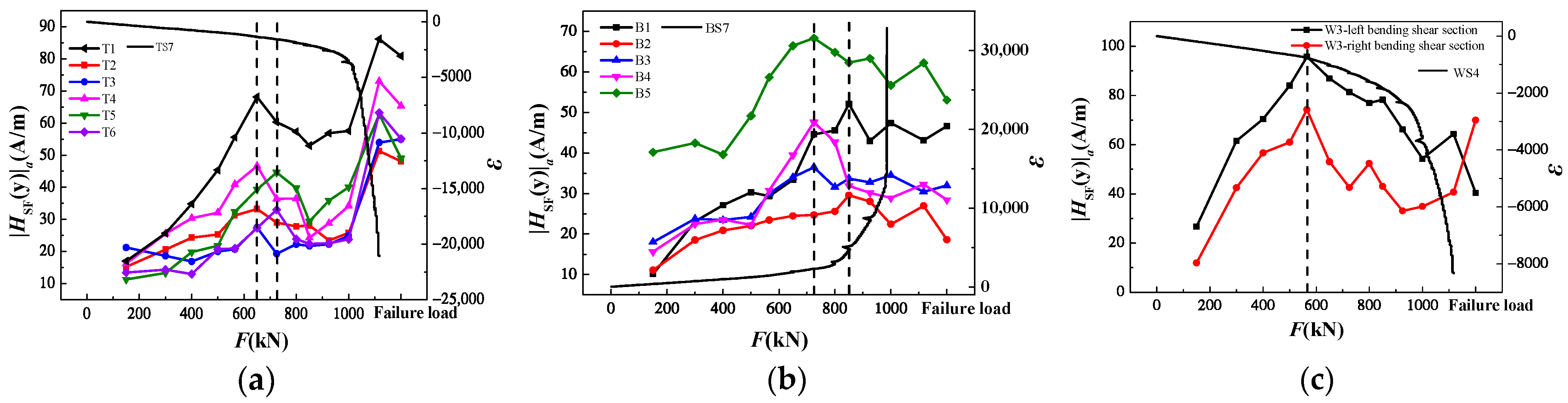
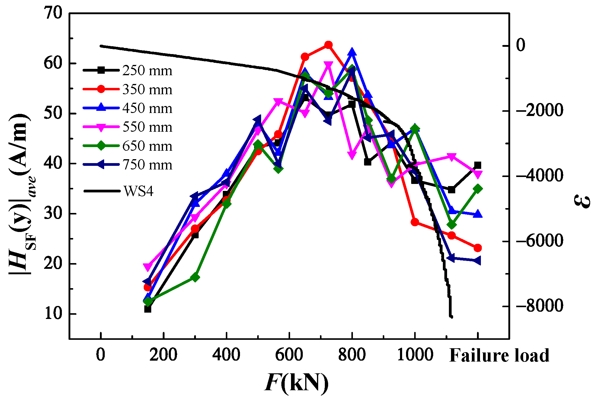
Through the peak distribution characteristics of the   Δ H SF ( y ) curve, the early SCZ of the steel box girder could be effectively identified and the buckling position could be predicted. For the SCZ caused by material discontinuity such as butt welds,   Δ H SF ( y ) extremum appeared on both sides of it.
(2)
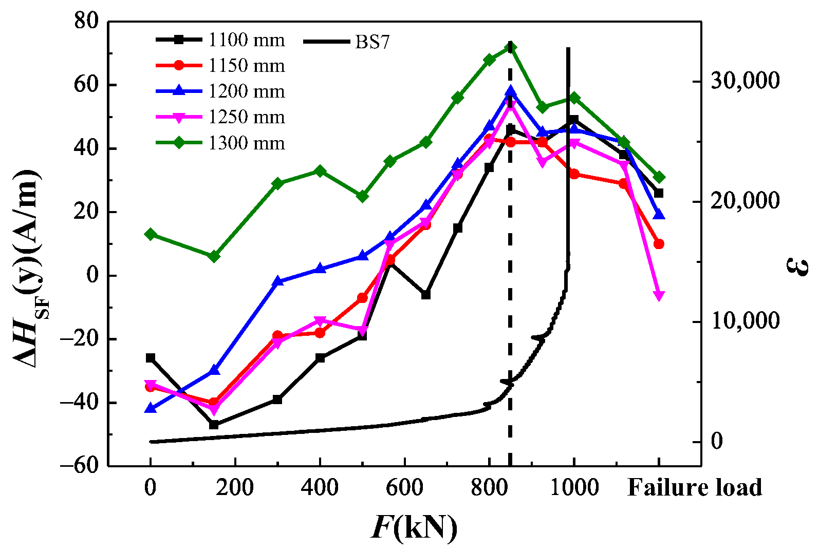
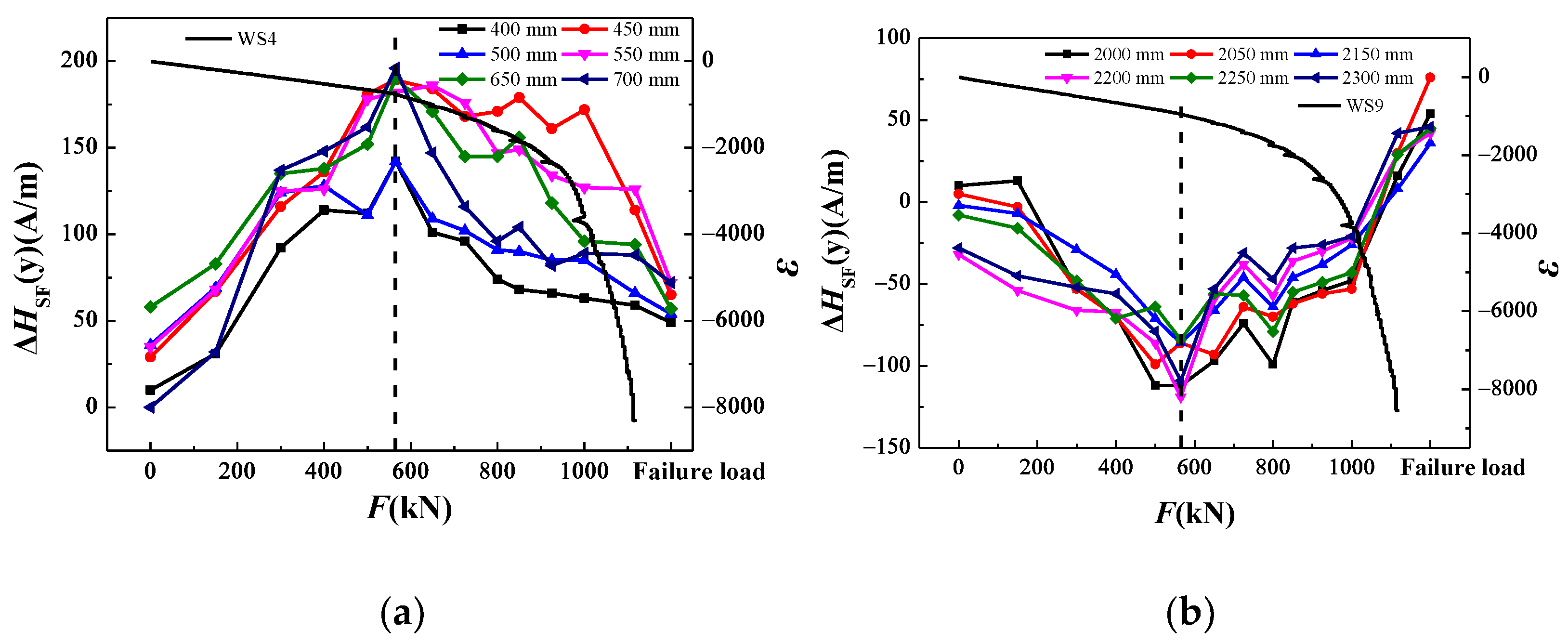
Whether it was the top and bottom flanges or the web, in engineering, the trend reversal of the   Δ H SF ( y ) -F curve could be used to detect whether each part was in the elastic-plastic working stage, and the magnetic characteristic parameter,   | H SF ( y ) | a   , further verified the accuracy of the results. This feature could be used as an early warning sign before the steel box girder was deformed or destroyed.
(3)
Through the reversal of the   | H SF ( y ) | a v e   -F curve, we could accurately judge the critical yield state of the web.
The fitted   | H SF ( y ) | a v e   -F linear expression could roughly quantify the shear capacity of the web. All the evaluation methods were expected to provide a basis for effectively evaluating the steel box girders with the MMMT method.

Author Contributions

Conceptualization, W.W. and F.Z.; methodology, S.S. and W.W.; validation, F.Z.; formal analysis, F.Z.; investigation, S.S.; resources, S.S. and W.W.; data curation, X.L. and J.L.; writing—original draft preparation, X.L. and J.L.; writing—review and editing, S.S. and W.W.; visualization, F.Z. and R.D.; supervision, R.D.; project administration, S.S. and W.W.; funding acquisition, S.S. and W.W. All authors have read and agreed to the published version of the manuscript.

Funding

This research was funded by the National Natural Science Foundation of China [grant numbers 51878548, 51478383] and the Key Project of Natural Science Basic Research Plan of Shaanxi Province [2018JZ5013, 2022JZ-21].

Data Availability Statement

The data used to support the findings of this study are available from the corresponding author upon request.

Conflicts of Interest

The authors declare no conflict of interest.

References

  1. Li, X.Y.; Zhang, G.; Kodur, V.; He, S.H.; Huang, Q. Designing method for fire safety of steel box bridge girders. Steel Compos. Struct. 2021, 38, 657–670. [Google Scholar]
  2. Gao, C.; Zhu, L.; Han, B.; Tang, Q.C.; Su, R. Dynamic Analysis of a Steel–Concrete Composite Box–Girder Bridge–Train Coupling System Considering Slip, Shear–Lag and Time–Dependent Effects. Buildings 2022, 12, 1389. [Google Scholar] [CrossRef]
  3. Li, L.F. The Analytieal Theory and Model Test Research on Local Stability of Orthotropie Steel Box Girder; Hunan University: Changsha, China, 2005. (In Chinese) [Google Scholar]
  4. Stamatelos, D.G.; Labeas, G.N.; Tserpes, K.I. Analytical calculation of local buckling and post–buckling behavior of isotropic and orthotropic stiffened panels. Thin–Walled. Struct. 2011, 49, 422–430. [Google Scholar] [CrossRef]
  5. Wang, F.; Lv, Z.D.; Zhao, Q.K.; Chen, H.L.; Mei, H.L. Experimental and numerical study on welding residual stress of U–rib stiffened plates. J. Construct. Steel Res. 2020, 175, 106362. [Google Scholar] [CrossRef]
  6. Wang, F.; Tian, L.J.; Lv, Z.D.; Zhao, Z.; Chen, Q.K.; Mei, H.L. Stability of full-scale orthotropic steel plates under axial and biased loading: Experimental and numerical studies. J. Construct. Steel Res. 2021, 181, 106613. [Google Scholar] [CrossRef]
  7. Wang, F.; Lv, Z.D.; Gu, M.J.; Chen, Q.K.; Zhao, Z.; Luo, J. Experimental study on stability of orthotropic steel box girder of self–anchored suspension cable–stayed bridge. Thin–Walled. Struct. 2021, 163, 107727. [Google Scholar] [CrossRef]
  8. Shi, P.P.; Su, S.Q.; Chen, Z.M. Overview of researches on the nondestructive testing method of metal magnetic memory, status and challenges. J. Nondestruct. Eval. 2020, 39, 1–37. [Google Scholar] [CrossRef]
  9. Shi, P.P.; Jin, K.; Zheng, X.J. A magnetomechanical model for the magnetic memory method. Int. J. Mech. Sci. 2017, 124, 229–241. [Google Scholar] [CrossRef]
  10. Shi, P.P.; Bai, P.G.; Chen, H.E.; Su, S.Q.; Chen, Z.M. The magneto-elastoplastic coupling effect on the magnetic flux leakage signal. J. Magn. Magn. Mater. 2020, 504, 166669. [Google Scholar] [CrossRef]
  11. Bao, S.; Jin, P.; Zhao, Z.; Fu, M. A Review of the Metal Magnetic Memory Method. J. Nondestruct. Eval. 2020, 39, 1–14. [Google Scholar] [CrossRef]
  12. Kashefi, M.; Clapham, L.; Krause, T.W.; Krause, P.; Ross, U.; Anthony, K.K. Stress–Induced Self–Magnetic Flux Leakage at Stress Concentration Zone. IEEE Trans. Magn. 2021, 57, 6200808. [Google Scholar] [CrossRef]
  13. Zhang, H.; Leng, L.; Zhao, R.Q.; Zhou, J.T.; Yang, M.; Xia, R.C. The non–destructive test of steel corrosion in reinforced concrete bridges using a micro–magnetic sensor. Sensors 2016, 16, 1439. [Google Scholar] [CrossRef] [PubMed] [Green Version]
  14. Roskosz, M.; Bieniek, M. Evaluation of residual stress in ferromagnetic steel based on residual magnetic feld measurements. NDT&E. Int. 2012, 45, 55–62. [Google Scholar]
  15. Roskosz, M.; Bieniek, M. Analysis of the universality of the residual stress evaluation method based on residual magnetic feld measurements. NDT&E. Int. 2013, 54, 63–68. [Google Scholar]
  16. Dong, L.H.; Xu, B.S.; Dong, S.Y.; Chen, Q.Z. Characterisation of stress concentration of ferromagnetic materials by metal magnetic memory testing. Nondestruct. Test. Eva. 2010, 25, 145–151. [Google Scholar] [CrossRef]
  17. Huang, H.H.; Jiang, S.L.; Yang, C.; Liu, Z.F. Stress concentration impact on the magnetic memory signal of ferromagnetic structural steel. Nondestruct. Test. Eval. 2014, 29, 377–390. [Google Scholar] [CrossRef]
  18. Bao, S.; Fu, M.L.; Lou, H.J.; Bai, S.Z.; Hu, S.N. Evaluation of stress concentration of a low-carbon steel based on residual magnetic field measurements. Insight 2016, 58, 678–682. [Google Scholar] [CrossRef]
  19. Dubov, A.A. Diagnostics of austenitic steel tubes in the superheaters of steam boilers using scattered magnetic fields. Therm. Eng. 1999, 46, 369–372. [Google Scholar]
  20. Liu, L.L.; Yang, L.J.; Gao, S.W. Propagation Characteristics of Magnetic Tomography Method Detection Signals of Oil and Gas Pipelines Based on Boundary Conditions. Sensors 2022, 22, 6055. [Google Scholar] [CrossRef]
  21. Shi, M.J.; Liang, Y.B.; Zhang, M.F.; Huang, Z.Q.; Feng, L.; Zhou, Z.Q. Pipeline Damage Detection Based on Metal Magnetic Memory. IEEE Trans. Magn. 2021, 57, 1–15. [Google Scholar] [CrossRef]
  22. Roskosz, M.; Rusin, A.; Kotowicz, J. The metal magnetic memory method in the diagnostics of power machinery component. J. Achiev. Mater. Manuf. Eng. 2010, 1, 362–370. [Google Scholar]
  23. Su, S.Q.; Zhao, X.R.; Wang, W.; Zhang, X.H. Metal Magnetic Memory Inspection of Q345 Steel Specimens with Butt Weld in Tensile and Bending Test. J. Nondestruct. Eval. 2019, 38, 64. [Google Scholar] [CrossRef]
  24. Su, S.Q.; Ma, X.P.; Wang, W.; Yang, Y.Y. Stress-dependent magnetic charge model for micro-defects of steel wire based on the magnetic memory method. Res. Nondest. Eval. 2020, 31, 24–47. [Google Scholar] [CrossRef]
  25. Li, M.L.; Yao, H.; Feng, J.R.; Yao, E.T.; Wang, P.; Shi, Y. Calculation and experimental verification of force-magnetic coupling model of magnetised rail based on density functional theory. Insight 2021, 63, 597–603. [Google Scholar] [CrossRef]
  26. Broniewicz, M.; Broniewicz, F. Welds assessment in k–type joints of hollow section trusses with I or H section chords. Buildings 2020, 10, 43. [Google Scholar] [CrossRef]
  27. Qiao, G.Y.; Liu, Y.M.; Han, X.L.; Wang, X.; Xiao, F.R. Simulation study on effects of geometry size of weld joint on bearing capacity of steel pipe. Trans. China Weld. Inst. 2017, 38, 33–36. [Google Scholar]
  28. Gorkunov, E. Different remanence states and their resistance to external effects. Discussing the “method of magnetic memory”. Russ. J. Nondestruct. 2014, 50, 617–633. [Google Scholar] [CrossRef]
  29. Gatelier–Rothea, C.; Chicois, J.; Fougeres, R.; Fleischmann, P. Characterization of pure iron and (130 P.P.M.) carbon–iron binary alloy by Barkhausen noise measurements, study of the influence of stress and microstructure. Acta. Mater. 1998, 46, 4873–4882. [Google Scholar] [CrossRef]
  30. Chen, X.; Liu, C.K.; Tao, C.H.; Dong, S.Y.; Wang, D.; Shi, C.L. Research on metal magnetic memory signal change of a ferromagnetic material under static tension. Nondestruct. Test. 2009, 31, 345–348. (In Chinese) [Google Scholar]
  31. Su, S.Q.; Yi, S.C.; Wang, W.; Sun, H.J.; Ren, G.C. Bending experimental study of structural steel beam on magnetic field gradient based on modified Jiles-Atherton model. Int. J. Appl. Electrom. 2017, 55, 409–421. [Google Scholar] [CrossRef]
  32. Guo, H.; Su, S.Q.; Wang, W.; Ma, X.P.; Yi, S.C.; Zhao, X.R. Relationship between applied force and magnetic field in a pseudo-static test of a portal frame. Int. J. Appl. Electrom. 2021, 66, 1–19. [Google Scholar] [CrossRef]
  33. Su, S.Q.; Qin, Y.L.; Wang, W.; Zuo, F.F.; Deng, R.Z.; Liu, X.W. Stress–magnetization of the state of flange damage to a bridge steel box beam based on magnetic memory inspection. Chin. J. Eng. 2022, 44, 900–910. (In Chinese) [Google Scholar]
  34. Yi, S.C.; Wang, W.; Su, S.Q. Bending experimental study on metal magnetic memory signal based on von Mises yield criterion. Int. J. Appl. Electrom. 2015, 49, 547–556. [Google Scholar] [CrossRef]
  35. Sablik, M.J.; Jiles, D.C. Coupled magnetoelastic theory of magnetic and magnetostrictive hysteresis. IEEE. Trans. Magn. 1993, 29, 2113. [Google Scholar] [CrossRef] [Green Version]
  36. Jiles, D.C.; Devine, M.K. Recent developments in modeling of the stress derivative of magnetization in ferromagnetic materials. J. Appl. Phys. 1994, 76, 7015. [Google Scholar] [CrossRef]
  37. Jiles, D.C. Theory of the magnetomechanical effect. J. Phys. D. Appl. Phys. 1995, 28, 1537. [Google Scholar] [CrossRef]
  38. Yang, E.; Li, L.M.; Chen, X. Magnetic field aberration induced by cycle stress. J. Magn. Magn. Mater. 2007, 312, 72–77. [Google Scholar]
  39. Cullity, B.D.; Graham, C.D. Introduction to Magnetic Materials; John Wiley Press: Hoboken, NJ, USA, 2008. [Google Scholar]
  40. Pitman, K.C. The influence of stress on ferromagnetic hysteresis. IEEE. Trans. Magn. 1990, 26, 1978–1980. [Google Scholar] [CrossRef]
  41. Bao, S.; Yang, J.; Gu, Y.B. Effect of strain rate history on the piezomagnetic field of ferromagnetic steels. J. Magn. Magn. Mater. 2021, 526, 167760. [Google Scholar] [CrossRef]
  42. Huang, H.H.; Qian, Z.C. Effect of Temperature and Stress on Residual Magnetic Signals in Ferromagnetic Structural Steel. IEEE Trans. Magn. 2017, 53, 6200108. [Google Scholar] [CrossRef]
  43. Zhao, X.R.; Su, S.Q.; Wang, W.; Zhang, X.H. Metal magnetic memory inspection of Q345B steel beam in four point bending fatigue test. J. Magn. Magn. Mater. 2020, 514, 167155. [Google Scholar] [CrossRef]
Figure 1. Schematic diagram of four-point bending loading of the specimen/unit: mm.
Buildings 12 01835 g001
Figure 2. A 3D model diagram of steel box girder/unit: mm.
Buildings 12 01835 g002
Figure 3. Cross-sectional dimension of the specimen/unit: mm.
Buildings 12 01835 g003
Figure 4. Layout diagram of inspection lines and strain gauges/unit: mm. (a) Top flange; (b) bottom flange; (c) one side of the web where the inspection lines were arranged; (d) one side of the web where the strain rosettes were arranged.
Buildings 12 01835 g004
Figure 5. Loading device and schematic diagram of the specimen.
Buildings 12 01835 g005
Figure 6. Load-displacement curve.
Buildings 12 01835 g006
Figure 7. EMS-2003 metal magnetic memory detector.
Buildings 12 01835 g007
Figure 8. Pen probe inspection.
Buildings 12 01835 g008
Figure 9. The final failure morphology of the specimen.
Buildings 12 01835 g009
Figure 10.   Δ H SF ( y ) curves of the top flange: (a) elastic and elastoplastic loading stages; (b) plastic deformation stage.
Buildings 12 01835 g010
Figure 11.   Δ H SF ( y )   curves of the bottom flange: (a) elastic loading stage; (b) elastoplastic and plastic deformation stages.
Buildings 12 01835 g011
Figure 12.   Δ H SF ( y )   curves of the web: (a) elastic and elastoplastic loading stages; (b) plastic deformation stage.
Buildings 12 01835 g012
Figure 13.   Δ H SF ( y ) -F relationship curves of the top flange: (a) non-SCZ location; (b) SCZ location.
Buildings 12 01835 g013
Figure 14.   Δ H SF ( y ) -F relationship curves of the bottom flange.
Buildings 12 01835 g014
Figure 15.   Δ H SF ( y ) -F relationship curves of the web: (a) left-bending shear section; (b) right-bending shear section.
Buildings 12 01835 g015
Figure 16.   |   H SF ( y ) | a -F relationship curves: (a) top flange; (b) bottom flange; (c) web.
Buildings 12 01835 g016
Figure 17. | H SF ( y ) | a v e -F relationship curves.
Buildings 12 01835 g017
Figure 18. | H SF ( y ) | a v e -F fitting curves.
Buildings 12 01835 g018
Publisher’s Note: MDPI stays neutral with regard to jurisdictional claims in published maps and institutional affiliations.

