Predicting the Geopolymerization Process of Fly-Ash-Based Geopolymer Using Machine Learning

Abstract

The process of geopolymerization affects the freshness and hardening properties of fly ash base polymer. The prediction of geological polymerization parameters, such as DPT, DPH, GPT, and GPH, is very important for the mixing optimization of FA base polymer. In this study, machine learning models such as backpropagation neural network, support vector regression, random forest, K-nearest neighbor, logistic regression, and multiple linear regression were used to predict the above geological polymerization parameters and explain the influence of composition on the geological polymerization of FA base polymer. Results show that RF was the most stable ML model and had the best predictive performance on the test sets of GPT, GPH, DPT, and DPH, with correlation coefficients of 0.88, 0.95, 0.92, and 0.95, respectively. The variable importance and sensitivity were analyzed by SHapley Additive exPlanations. Results indicate that temperature is the most significant input variable affecting the DPT, DPH, and GPH with SHAP values of 0.09, 4.83, and 1.03, respectively. For GPT, the SHAP value of temperature is 6.89, slightly lower than that of LFR (6.95); yet it is a still significantly important input variable. The mole ratio and alkaline solution concentration were also important and negatively contributed to DPT and DPH, respectively. Besides, both GPT and GPH were sensitive to the mass ratio of liquid-to-fly ash which can promote the geopolymerization extent and shorten the geopolymerization time at a small content. The results of this study pave the way for automatic mixture optimization of FA-based geopolymers.

1. Introduction

Cement is a vital component of concrete and the most widely used manmade material on the planet [1]. However, cement production accounts for as much as 7% of global CO₂ emissions [2] and 12–15% of the world’s industrial energy use [3]. To protect the environment, eco-friendly binder materials that can replace cement in concrete are urgently needed. Geopolymer is one of the most important alternatives to cement. Geopolymers are developed from industrial wastes containing pozzolanic minerals. Therefore, geopolymers have a large number of advantages such as lower cost, higher mechanical strength, excellent fire, and corrosion resistance, and lower energy consumption [4]. Besides, it has a reduced carbon footprint compared to cement [5]. The CO₂ emission may be reduced by 60–80% if the cement is replaced by geopolymer in construction materials [6].

Geopolymers are synthesized using a variety of feedstocks with different chemical compositions. According to the different content of calcium oxide in raw materials, geopolymers are generally divided into low calcium type and high calcium type. Metakaolin and fly ash are representative materials of low-calcium geopolymer, which usually need to be synthesized with high alkalinity hydroxide or alamu metalosilicate solution [7]. In the process of geodetic polymerization, the SiO₄ tetrahedron and AlO₄ tetrahedron are formed in the process of dissolution, diffusion, condensation, and dehydration hardening of Si-Al components in the raw material. The representative materials of high calcium geopolymer are furnace slag and steel slag with high calcium oxide content. These materials can be activated by hydroxide and silicate as well as alkali metal carbonate and sulfate solutions.

Among all the raw materials, FA is one of the most commonly used waste materials as it is readily available and cheap [8], and consists of a high amount of aluminum and silicon [9]. FA is produced by burning pulverized coal in coal-fired power plants. The types, amounts, and proportions of different minerals in FA depend on the type of coal burned. The physical and chemical characteristics of FA depend to a large extent on the source of coal, degree of pulverization, combustion conditions, ash collection, plant treatment, and disposal methods, respectively [10]. According to the American Society for Testing and Materials standards, C618 FA can be classified as C and F based on its calcium oxide content. Type C FA has a high calcium content and is mainly produced by the combustion of lignite sources. The content of total SiO₂, Al₂O₃, and Fe₂O₃ in class C FA is between 50 and 70 wt.%, and the content of CaO is more than 20 wt.%. Class F FA has a low calcium content and is produced by burning anthracite or bituminous coal. The total content of SiO₂, Al₂O₃, and Fe₂O₃ of type F FA is more than 70 wt.%, and the content of CaO is less than 10%. High calcium FA base polymers can set and harden very rapidly without any thermal curing [11]. The setting time of the base polymer of low-calcium fly ash is slow, so it needs to be heated to accelerate the hardening process [12].

The synthesis of FA-based geopolymers involves heterogeneous chemical reactions called geopolymerization reactions. Geopolymerization is a complicated process that consists of multiple steps including leaching, diffusion, reorientation, polymerization, and condensation [13]. During geopolymerization, the particles of the aluminosilicate materials will be attacked by hydroxide ions once the alkali solution is mixed with the aluminosilicate materials. This attack will break the Si–O, and Al–O bonds of the aluminosilicate materials and form aluminate and silicate monomers. The increase of these monomers will lead to the formation of the 3D aluminosilicate gel network [4].

The geopolymerization of the FA-based geopolymers is controlled by several parameters such as the mole ratio (MR), the alkaline solution concentration (ASC), the liquid-to-fly ash mass ratio (LFR), and the curing temperature (T). The recommended MR, ASC, LFR, and T were 1.0–2.0 M, 15–25%, 0.3–0.45, and 50–80 °C, respectively, according to the previous literature [14]. These parameters significantly influence the fresh and hardened properties of the FA-based geopolymers [15], and hence it is of considerable importance to predict the geopolymerization parameters and interpret the influence of mixture proportions on these parameters.

Several experimental methods have been used to characterize the geopolymerization process. Among them, X-ray diffraction is usually employed to test the crystallization behavior of the geopolymerization process during the reaction but can only provide very limited information [16]. Energy-dispersive X-ray diffraction is a new approach to recording the kinetics of geopolymerization; however, it is only valid for the initial setting period [17]. Other characterization methods such as environmental scanning electron microscopy, ²⁷Al/²⁹Si Nuclear Magnetic Resonance, etc., are also able to characterize geopolymerization [18]. Nonetheless, all the above methods intermittently record the geopolymerization process and cannot provide real-time geopolymerization parameters. Different from the above methods, calorimetric characterization technology can obtain geopolymerization parameters in real-time during the entire process of geopolymerization, which has irreplaceable advantages over other methods of recording to understand the degree and rate of geopolymerization [19]. Therefore, the geopolymerization peak time (DPT), peak heat of dissolution (DPH), the peak time of geopolymerization (GPT), and peak heat of geopolymerization (GPH) obtained by calorimetry were analyzed in this study.

The above-mentioned geopolymerization parameters should be predicted in advance to provide information for the mixture design of FA-based geopolymers. However, few prediction models are proposed in the literature. In recent years, the use of machine learning (ML) has been considered a powerful tool for predicting the performance of cementitious materials [20]. Due to the excellent fitting capability of ML, the output can be accurately predicted when the input variables are highly uncorrelated, reducing the need for time-consuming and expensive experiments [21]. Therefore, this study adopted ML models to evaluate geopolymerization parameters (DPT, DPH, GPT, GPH). However, there is no single best ML model for every dataset as per the no-free-lunch theorem [22]. Therefore, evaluation of the performance of different ML models is of vital importance to select a model with the best prediction performance. It should also be noted that for the ML models to have robust performance, we need to optimize their hyperparameters. Metaheuristics have the advantages of simple coding and high computational efficiency, which can be used as optimization algorithms for hyperparameter tuning [23]. In recent years, an individual intelligence-based beetle antenna search algorithm (BAS) has been proposed [24]. The BAS algorithm has simple code and is easy to implement, and also, its calculation time is very short. At the same time, due to its specific step size strategy, it can overcome the shortcoming of falling into the local optima [25]. Therefore, this paper uses the BAS algorithm to optimize the hyperparameters.

We aim to accurately predict the geopolymerization parameters and interpretate the influence of geopolymer composition on its geopolymerization process. This paper adopts machine learning methods to model the geopolymerization parameters of the FA-based geopolymer. In the following parts, Section 2 describes the dataset, the construction of the ML model, and the principle of the BAS algorithm. Then, in Section 3, the results of hyperparameter tuning were summarized and the performance of different ML algorithms was compared. Finally, the ML model was used to study the importance and sensitivity of the variables. The RF model can be used to evaluate the effects of mixing parameters (molar ratio, alkaline solution concentration, liquid–cement mass ratio) and temperature on the FA-based polymerization process more effectively. This model can further reduce the trial and error in the process of mix ratio design and can be used to study the sensitivity of mix ratio design parameters. The information obtained from this model can be used as a guide for the mixing optimization of FA-based polymers.

2. Methodology

2.1. Dataset

The geopolymerization parameters of FA-based geopolymers were characterized by the isothermal calorimetry method [16]. In a typical calorimetric curve, the first exothermal peak (the dissolution peak) with high intensity appeared very fast after the fly ash initially contacted the alkali activator, indicating a very high dissolution rate of the fly ash. After this, the dissolution peak suddenly dropped, while the mixture continued to release heat, and a second flat and wide exothermic peak appeared, which was called the geopolymerization peak [26]. This peak provided information on the strength development of the geopolymer. The intensity and appearance time of these peaks on the calorimetric curve was very important to the fresh and hardened properties of geopolymers. Therefore, it is important to predict the dissolution peak time (DPT), dissolution peak heat (DPH), geopolymerization peak time (GPT), and geopolymerization peak heat (GPH) during geopolymerization for mixture optimization [26].

In the present research, the dataset was derived from previous literature [26,27]. The dataset includes 72 experimental results of DPT, DPH, GPT, and GPH, respectively. In this dataset, fly ash with a ratio of 2.52 and fineness of 419.6 m²/kg was used as the precursor material. The chemical analysis of fly ash is given in

Table 1. Chemical analysis of fly ash.

LOI	K2O	Na2O	MgO	CaO	SO3	Fe2O3	Al2O3	SiO2	Others
0.49	0.27	2.97	6.74	28.8	3.47	6.8	16	30.7	3.28

Note: All values are mass %; LOI is the ignition loss at 1000 °C.

.

NaOH and Na₂SiO₃ were used as activators. By adjusting the content of NaOH in the NaOH-Na₂SiO₃ solution, the SiO₂/Na₂O molar ratio of the designed alkali solution is 1.0, 1.5, and 2.0. The alkaline solution was diluted with deionized water and adjusted the concentration of the alkaline solution to 15%, 20%, and 25% (by mass). Fly ash and nine alkali solutions were mixed according to the liquid–cement ratio (L/F = 0.33, 0.40, 0.50, 0.60). The mixture design is shown in

Table 2. Design of the geopolymer mixture.

Mole Ratio	Alkaline Solution Concentration (%)	L/F
2.0	25	0.6, 0.5, 0.4, 0.33
2.0	20	0.6, 0.5, 0.4, 0.33
2.0	15	0.6, 0.5, 0.4, 0.33
1.5	25	0.6, 0.5, 0.4, 0.33
1.5	20	0.6, 0.5, 0.4, 0.33
1.5	15	0.6, 0.5, 0.4, 0.33
1.0	25	0.6, 0.5, 0.4, 0.33
1.0	20	0.6, 0.5, 0.4, 0.33
1.0	15	0.6, 0.5, 0.4, 0.33

.

This component includes molar ratio (MR), alkaline solution concentration (ASC), and liquid–cement mass ratio (LFR). Curing temperature (T) has a significant effect on the process of geodetic polymerization. Therefore, the component parameters MR, ASC, and LFR and the environmental parameter T are used as input variables. The higher the molar ratio, the higher the concentration of free silicate ions in the alkali solution, which may form geopolymerization products on the surface of FA particles in a short time and inhibit the further dissolution of FA [28]. The liquid FA ratio has an important effect on the degree and time of geopolymerization. The concentration of alkaline solution has a great influence on the dissolution of FA in alkaline solution. Temperature affects the kinetic energy of the FA base polymer, which is conducive to the breaking and formation of solute molecular bonds [29].

The correlation coefficients between each input variable are shown in the matrix of correlation coefficients (Figure 1). The Pearson correlation coefficient between two different variables was less than 0.5, which indicates that there was no multi-collinearity problem between these input variables [30]. The statistical description of the variables was shown in

Table 3. Statistical description of the input parameters.

Variable	Unit	Mean	STD	Min	25%	50%	75%	Max
MR	-	1.50	0.41	1.00	1.00	1.50	2.00	2.00
ASC	%	20.00	4.11	15.00	15.00	20.00	25.00	25.00
LFR	-	0.46	0.10	0.33	0.38	0.45	0.53	0.60
T	°C	36.88	13.59	23.00	23.00	50.00	50.00	50.00
DPT	h	0.29	0.13	0.13	0.20	0.28	0.35	0.73
DPH	mw	8.64	5.54	0.81	3.68	8.44	14.10	17.30
GPT	h	15.03	22.37	1.05	2.84	6.76	14.79	116.15
GPH	mw	2.23	1.43	0.28	0.98	1.81	3.31	5.43

.

2.2. Machine Learning Approaches

2.2.1. Backpropagation Neural Networks (BPNN)

The backpropagation neural network (BPNN) has been widely employed to solve engineering issues [31]. The architecture of BPNN is composed of the input, output, and several hidden layers. This algorithm compares the differences between the predicted and actual outputs during the training process to calculate the errors which then propagates backward to minimize the weights and thresholds. The prediction accuracy of BPNN can be significantly improved by the backpropagation process. Figure 2 presents a representative structure of the BPNN model. In this figure, X is the input neuron, H is the hidden neuron, and Y is the output neuron.The equation shown as follows can be employed to determine the correlation between the output variable and inputs of a neuron in the BPNN.

$$O=f\left({{\displaystyle \sum }}_{i=1}^m{w}_j{x}_j+b\right)$$

(1)

In which $O$ denotes the neuron output; $f$ is an activation function for restricting the amplitude of the output; $w_j$ denotes the weight of the input $x_j$; b can represent the value of bias in the neuron. The sigmoid function can be usually used as the function of activation as follows:

$$f\left(x\right)=\frac{2}{1+\exp \left(-x\right)}-1$$

(2)

The mean square error (MSE) can be employed as the threshold to terminate the training process:

$$MSE=\frac{1}{n}{{\displaystyle \sum }}_{i=1}^n{\left(y_i-{\widehat{y}}_i\right)}^2$$

(3)

where $y_i$ is the actual value of the output; ${\widehat{y}}_i$ is the predicted value of the output.

2.2.2. Support Vector Regression (SVR)

Support vector regression (SVR) is a popular supervised algorithm based on a machine learning approach [32]. This algorithm can model the correlation between the input parameters and output parameters by mapping the data into a characteristic space with higher dimensions from the sample space. The separation of training data can be maximized and the upper bound of errors can be minimized by SVR. It is broadly employed because it has a fast-learning speed, an outstanding generalization capability, and is not sensitive to noise. Figure 3 plots a schematic diagram of a SVR model. In this figure, the bule stars represent the data points in the dataset.

Generally, the following equation is applied to describe the SVR model:

$$f\left(x\right)=w·\phi \left(x\right)+b$$

(4)

where x is an l-dimensional input variable; $w$ represents the weight vector; $\phi \left(x\right)$ denotes a nonlinear mapping function; b is the deviation value. The loss function $ℒ$ for the SVR algorithm is defined as follows:

$$ℒ\left(x,y,f\right)={\left|y_i-f\left(x_i\right)\right|}_{\epsilon }=\{\begin{array}{c}0,\left|y_i-f\left(x_i\right)\right|<\epsilon \\ \left|y_i-f\left(x_i\right)\right|-\epsilon , \left|y_i-f\left(x_i\right)\right|\ge \epsilon \end{array}$$

(5)

where $y_{\mathrm{i}}$ is the actual value of the output of $x_i$; $f\left(x_i\right)$ is the predicted value of the output of $x$; $\epsilon$ is the maximum tolerance error. It should be noted that only the points situated on or outside the $\epsilon$-tube can be employed as support vectors to build $f\left(x\right)$. The problem can be re-expressed to minimize the structural risk:

$$ℛ\left(w\right)=\frac{1}{2}||w{||}^2+{\displaystyle \sum }_{i=1}^nℒ\left(x,y,f\right)$$

(6)

The above equation is transferred as the convex optimization problem by describing the slack variables ${\xi }_i$ and ${\xi }_i^{*}$:

$$mi{n}_{w,b,\xi ,{\xi }^{*}}ℛ\left(w\right)=\frac{1}{2}||w{||}^2+C{\displaystyle \sum }_{i=1}^n\left({\xi }_i+{\xi }_i^{*}\right)s.t.$$

$$s.t.\{\begin{array}{c}{\mathrm{y}}_i-\mathbf{w}·\phi \left(x\right)-b\le \epsilon +{\xi }_i\\ \mathbf{w}·\phi \left(x\right)+b-{\mathrm{y}}_i\le \epsilon +{\xi }_i^{*}\\ {\xi }_i\ge 0\\ {\xi }_i^{*}\ge 0\end{array}$$

(7)

in which C is a penalty argument for determining the trade-off between the degree of punishment of the data outside the tube and the flatness of $f\left(x\right)$.

The constraint problem can be solved by introducing the Lagrange multipliers:

$$L\left(w,b,\xi ,\alpha ,\mu \right)=\frac{1}{2}||w{||}^2+C{\displaystyle \sum }_{i=1}^n\left({\xi }_i+{\xi }_i^{*}\right)$$

$$-{\displaystyle \sum }_{i=1}^n{\alpha }_i\left(\epsilon +{\xi }_i-{\mathrm{y}}_i+w·\phi \left(x_i\right)+b\right)$$

$$-{\displaystyle \sum }_{i=1}^n{\alpha }_i^{*}\left(\epsilon +{\xi }_i^{*}+{\mathrm{y}}_i-w·\phi \left(x_i\right)-b\right)$$

$$-{\displaystyle \sum }_{i=1}^n\left({\mu }_i{\xi }_i+{\mu }_i^{*}{\xi }_i^{*}\right)$$

(8)

where ${\alpha }_i\ge 0$, ${\alpha }_i^{*}\ge 0$, ${\mu }_i\ge 0$ and ${\mu }_i^{*}\ge 0$ are Lagrange multipliers. The Karush–Kuhn-Tucker (KKT) conditions must be satisfied when the objective function is differentiable and the constraint functions have strong duality:

$$\{\begin{array}{c}\frac{\partial L}{\partial w}=\mathbf{w}-{\displaystyle \sum }_{i=1}^n\left({\alpha }_i-{\alpha }_i^{*}\right)\phi \left(x_i\right)=0\\ \frac{\partial L}{\partial \mathrm{b}}={\displaystyle \sum }_{i=1}^n\left({\alpha }_i-{\alpha }_i^{*}\right)=0\\ C-{\alpha }_i-{\mu }_i=0\\ C-{\alpha }_i^{*}-{\mu }_i^{*}=0\end{array}$$

(9)

Besides, at the optimal solution, the following equations should be zero based on KKT conditions:

$$\{\begin{array}{c}{\alpha }_i\left(\epsilon +{\xi }_i-{\mathrm{y}}_i+w·\phi \left(x_i\right)+b\right)=0\\ {\alpha }_i^{*}\left(\epsilon +{\xi }_i^{*}+{\mathrm{y}}_i-\mathbf{w}·\phi \left(x_i\right)-b\right)=0\\ \left(C-{\alpha }_i\right){\xi }_i=0\\ \left(C-{\alpha }_i^{*}\right){\xi }_i^{*}=0\end{array}$$

(10)

The Lagrange dual problem is then addressed by substituting the above equations

$$\begin{gathered} \underset{i}{\max }\left(-\frac{1}{2}{\displaystyle \sum }_{i=1}^n{{\displaystyle \sum }}_{j=1}^n\left({\alpha }_i-{\alpha }_i^{*}\right)\left({\alpha }_j-{\alpha }_j^{*}\right)x_i^T{x}_j-\epsilon {{\displaystyle \sum }}_{i=1}^n\left({\alpha }_i+{\alpha }_i^{*}\right) \\ +{{\displaystyle \sum }}_{i=1}^n{y}_i\left({\alpha }_i-{\alpha }_i^{*}\right)\right)s.t.\{\begin{array}{c}{{\displaystyle \sum }}_{i=1}^n\left({\alpha }_i-{\alpha }_i^{*}\right)=0\\ {\alpha }_i,{\alpha }_i^{*}ϵ\left[0,C\right]\end{array} \end{gathered}$$

(11)

The SVR model can be reiterated as follows by substituting w = ${\displaystyle \sum }_{i=1}^n\left({\alpha }_i-{\alpha }_i^{*}\right)\phi \left(x_i\right)$:

$$f\left(x\right)={{\displaystyle \sum }}_{i=1}^n\left({\alpha }_i-{\alpha }_i^{*}\right)\phi \left(x_i\right)x+b$$

(12)

2.2.3. Random Forest (RF)

Random Forest (RF) is a supervised machine learning algorithm made up of decision trees using both bagging and feature randomness [33]. The bagging method repeatedly samples the original training set and produces many new training sets. The weak tree models are then trained on these newly generated training sets. The feature randomness is the selection of a random characteristic subset at each node of the tree.

A typical flowchart of the RF structure is plotted in Figure 4. The construction procedure of the RF model can be iterated as follows:

$X=\left\{x_1,x_2,\dots ,x_n\right\}$ is the original training set with n samples and its label is $Y=\left\{y_1,y_2,\dots ,y_n\right\}$. The data in the original training set is then randomly sampled with replacement to generate N new training sets $\left\{X_1,X_2,\dots ,X_n\right\}$ with labels $\left\{Y_1,Y_2,\dots ,Y_n\right\}$.

The N decision trees $\left\{t_1,t_2,\dots ,t_N\right\}$ are grown on newly generated training sets by randomly selecting characteristics at every node of the tree without pruning.

The plurality of the voting rule is used to aggregate the outcomes of all decision trees.

2.2.4. The k-Nearest Neighbor

The k-nearest neighbor (kNN) algorithm is also a widely used algorithm for solving regression and classification algorithms. This algorithm compares determines the label of new data by comparing the labels of the k closest data [34]. The Minkowski metric is generally employed to define the distance between input vectors $x_i$ and $x_j$:

$$||x_i-x_j{||}^p={({\displaystyle \sum }_{i=1}^q{\left|x_i-x_j\right|}^p)}^{1/p}$$

(13)

The predicted output can be represented by the following equation:

$$\widehat{y}=\frac{1}{k}{{\displaystyle \sum }}_{i=1}^k{y}_i$$

(14)

where $y_i$ is the distance $d_i$ between $x$ and the ith sample. Finally, the predicted value $\widehat{y}$ is the mean of the predicted value of its k nearest neighbors.

2.2.5. Logistic Regression

Logistic regression (LR) is a popular ML model that utilizes logistic functions to model dependent variables. An LR model with multiple predictors can be represented by the following equation:

$$ln\frac{p}{1-p}=b_0+{{\displaystyle \sum }}_{k=1}^n{b}_k{x}_k$$

(15)

where p is a dependent variable as a probability; b₀,..., b_n denote the constant coefficients of the LR model; x₁,..., x_n represent the independent variables.

2.2.6. Multiple Linear Regression

Multiple linear regression (MLR) uses the following linear equations to model the input-output correlation:

$$Y={\beta }_0+{\beta }_1{X}_1+{\beta }_2{X}_2+\dots +{\beta }_n{X}_n$$

(16)

where $X$ represents an n-dimensional feature vector; ${\beta }_i\left(i=1,2,\dots n\right)$ represents the regression coefficients, and Y is the output variable.

2.3. Optimization Algorithm

In this study, the beetle antennae search (BAS) algorithm is employed to tune the hyperparameters of the ML models. This algorithm is inspired by the beetle’s foraging behavior. A beetle search for food using its two antennae. The beetle’s movement direction depends on the concentration of the odor. Assume that b is a random vector representing the direction, which is defined as:

$$\mathit{b}=\frac{rand\left(k,1\right)}{rand\left(k,1\right)}$$

(17)

where $rand$ is a uniform random function and $k$ represents the dimension of the searching space. The position vector can be written as:

$$x_r^i=x^i+d^i\mathit{b}$$

(18)

$$x_l^i=x^i-d^i\mathit{b}$$

(19)

where $x^i$ is the beetle position at the $i^{th}$ time instant (i = 1, 2…); $d^i$ is the distance between the antennas at the $i^{th}$ time instant; $x_r^i$ and $x_l^i$ represent a position on the right and left antennae side at the $i^{th}$ time instant, respectively.

The beetle’s position vector is updated according to the following equation:

$$x^i=x^{i-1}+{\delta }^i\mathit{b}sign(f\left(x_r^i\right)-f\left(x_l^i\right))$$

(20)

where ${\delta }^i$ is the step size at time $i$; $f\left(x\right)$ is the objective function. The following updating strategy for the antennae length and step size can be applied to avoid being trapped into local optima:

$${\delta }^i=0.95{\delta }^{i-1}$$

(21)

$$d^i=0.95d^{i-1}+0.01$$

(22)

The flow chart of the tuning ML model using BAS is shown in Figure 5.

2.4. K-Fold Cross Validation

When the dataset is small, the overfitting problem easily occur. To prevent this problem, K-fold cross-validation (CV) was introduced [35]. As suggested above, the value of k is set to 10. Specifically, the dataset is randomly divided into a training set (external training set) containing 80% of the instances and a test set containing 20% of the instances. The external training set is further divided into 10 subsets. In each fold, the BAS algorithm searches for the optimal hyperparameter on nine subsets and then calculates the root mean square error (RMSE) on another validation set, as shown in Figure 6. This process is repeated 10 times, each time using a different set as the validation set. After 10 times of cross-validation, the 10 groups of hyperparameters were averaged to obtain the final result.

2.5. Evaluation of the Predicted Results

The predicted results of ML models to estimate geopolymerization parameters were assessed using the root-mean-square error (RMSE) and correlation coefficient (R).

RMSE refers to the deviation between the evaluated and target values. It is given by:

$$RMSE=\sqrt{\frac{1}{n}{{\displaystyle \sum }}_{i=1}^n{\left(y_i^{*}-y_i\right)}^2}$$

(23)

where $y_i$ denote the actual value; $y_i^{*}$ denote the predicted value; $n$ is the number of instances.

R expresses the strength of correlation between predicted and observed values. It is expressed as:

$$R=\frac{{{\displaystyle \sum }}_{i=1}^n\left(y_i^{*}-{\overline{y}}^{*}\right)\left(y_i-\overline{y}\right)}{\sqrt{{{\displaystyle \sum }}_{i=1}^n{\left(y_i^{*}-{\overline{y}}^{*}\right)}^2}\sqrt{{{\displaystyle \sum }}_{i=1}^n{\left(y_i-\overline{y}\right)}^2}}$$

(24)

where ${\overline{y}}^{*}$ is the average value of the predicted results; $\overline{y}$ is the average value of the actual results; n presents the instance number.

3. Results and Discussion

3.1. Evaluation of the Hyperparameter Tuning

As mentioned previously, BPNN, SVR, RF, kNN, LR, and MLR were used to predict the DPT, DPH, GPT, and GPH. These algorithms were trained on the training set including 80% of the dataset samples and tested on the testing dataset containing 20% of the data. First of all, this study used BAS combined with 10-fold cross-validation to obtain the optimized hyperparameters. Then, the obtained 10 optimal hyperparameters were averaged to obtain the final result. Figure 7 shows the RMSE change with iteration for the ML models during hyperparameter tuning on the fold with the lowest RMSE. It can be seen that all the RMSE curves converge in the first 50 iterations, which indicates that BAS has a good performance in finding the optimal hyperparameters of the ML model. Different ML algorithms presented different RMSE-change patterns in terms of the convergence velocity and final RMSE values. For all predicted target variables, kNN took the shortest time to reach convergence due to its simple structures and hyperparameters compared with other ML algorithms. It can be also seen that SVM reached convergence with the lowest RMSE on the DPH, GPT, and GPH sets, while on the DPT dataset, although BPNN took the longest time to achieve convergence, it had the lowest RMSE after convergence. It is interesting to note that the RMSE of SVR and KNN decreased marginally when tuning hyperparameters on the GPT dataset, which means that the initial values of the hyperparameters were approximate to the optimal values. The obtained optimal hyperparameters of each model can be found in

Table 4. Optimal hyperparameters used in this study for each ML model.

Data Set	Model	Hyperparameter
DPT	BPNN	layer_num = 3; neuron_num = [20 8 1]
	SVR	C = 1.26; γ = 0.8
	RF	min_samples_leaf = 2; tree_num = 57
	KNN	neighbor_num = 1
	RF	min_samples_leaf = 1; tree_num = 6
	MLR	-
DPH	BPNN	layer_num = 3; neuron_num = [7 5 10]
	SVR	C = 6.54; γ = 20.4
	KNN	neighbor_num = 1
	LR	-
	RF	min_samples_leaf = 1; tree_num = 27
GPT	BPNN	layer_num = 2; neuron_num = [20 3]
	SVR	C = 12.1; γ = 7.9
	KNN	neighbor_num = 13
	LR	-
	MLR	-
GPH	RF	min_samples_leaf = 1; tree_num = 27
	SVR	C = 24.1; γ = 6.4
	KNN	neighbor_num = 1
	LR	-
	MLR	-

.

3.2. Prediction Performance of ML Models

In this section, the performance of each computational model is evaluated by calculating the RMSE and R values on the test set, as shown in Figure 8. It can be clearly observed that RF has better prediction performance than the other models in terms of minimum RMSE (0.06, 2.3, 7.5, and 0.65 for DPT, DPH, GPT and GPH, respectively) and highest R (0.92, 0.95, 0.88, 0.95 for DPT, DPH, GPT and GPH, respectively). The possible reason is that the RF model creates an uncorrelated forest of decision trees using both bagging and feature randomness, which helps to decrease the model’s variance than other single models like BPNN, SVM. KNN, etc. It can be also noted that for prediction of DPT, DPH, GPT and GPH, the methods with the worst predicting effect regarding R and RMSE are LR (0.67 and 0.16, respectively), BPNN (0.78 and 4.4, respectively), MLR (0.35 and 22.2, respectively) and LR (0.62 and 0.67, respectively). This indicates that simple regression models such as LR and MLR are unable to simulate the highly nonlinear relationship between geopolymer composition and geopolymer parameters. Figure 9 shows the relationship between the predicted and actual values on both RF sets. It can be seen that most of the values are near the ideal fitting line (R = 1) except for a few outliers, which may be caused by insufficient training data in these areas. Therefore, RF is recommended as the best model to predict the parameters of FA-based polymers.

Ling et al. [36] also used artificial neural network (ANN) models to predict GPH. The R value of this model is 0.959, which is similar to the R value of this study (0.95). However, other geological aggregation parameters, including GPT, DPT, and DPH, were not considered in the previous study. Compared with the previous studies, the prediction of parameters and the important variables affecting the process of geological polymerization were comprehensively explained in this study.

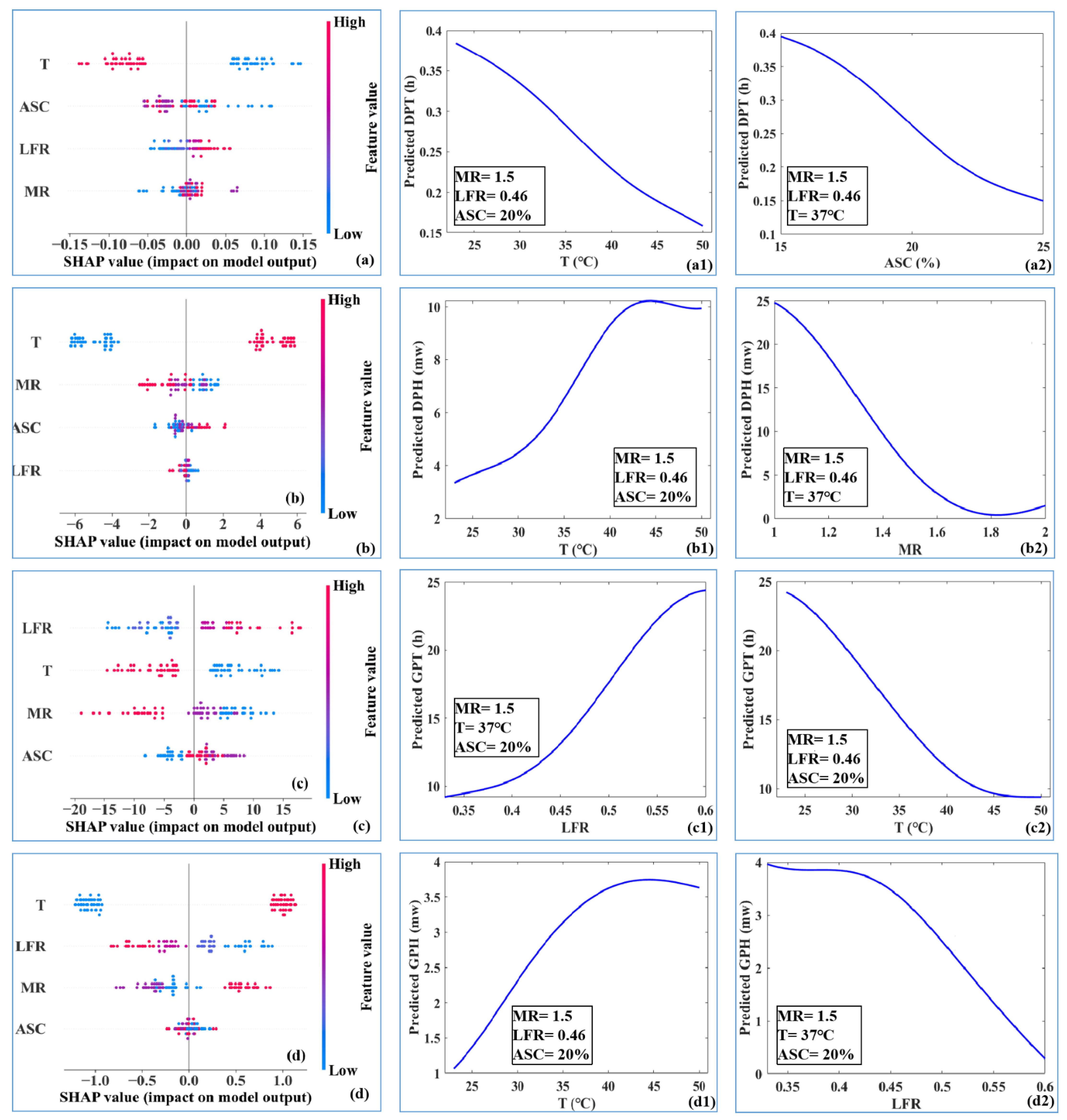
3.3. Importance of the Input Variables

ML models such as RF have a non-linear and highly complex architecture, and therefore they tend to behave as a black-box model. Tree-like models are interpretable due to their hierarchical structure, but the visualization of these models may not be easy to interpret. To address the interpretability problem of RF models, a useful agnostic tool, i.e,: Shapley additive explanations (SHAP) was introduced to explain the highly complex RF algorithms with a large number of parameters [37]. For RF, a SHAP approximation method called TreeExplainer was used in this study.

TreeExplainer is a package for explaining and interpreting predictions of tree-based ML models. The basic idea is to decompose each prediction into feature contribution components. For a dataset with n features, each prediction on the dataset is calculated as

$$y_i=y_{base}+f\left(x_{i1}\right)+f\left(x_{i2}\right)+\dots +f\left(x_{ik}\right)$$

(25)

where $y_i$ is the prediction value of each sample; $y_{base}$ is the baseline representing the mean of all output variables; $f\left(x_{ik}\right)$ is the contribution of the kth feature of Sample i.

Figure 10 shows the mean SHAP values of different input features for the four geopolymerization parameters. Different features were sorted in descending order of importance. It is observed that T is the most important input parameter affecting the DPT, DPH, and GPH with SHAP values of 0.09, 4.83, 1.03, respectively. For GPT, the SHAP value of T is 6.89, slightly lower than that of LFR (6.95); yet it is a still significantly important input variable. This may be because the higher temperature increases the kinetic energy of the system, which promotes the bond breaking and formation of solute molecules [38].

3.4. Sensitivity Analysis

Figure 11 gives the influences of the top features on the output of the model. A single dot represents an instance on each feature row. The SHAP value determines the horizontal position of the points, which are “stacked” along each feature row to show density. The importance of the features was arranged in descending order. The sensitivity of the two most important input variables to the outputs was analyzed by the trained ML model (see the blue lines in Figure 11). In detail, we changed the variable to be analyzed and fixed the other variable to their mean values and then predicted the output using the trained ML model. It can be seen that low temperature corresponded to higher SHAP values for DPT (Figure 11a) and GPT (Figure 11b), and lower SHAP values for DPH (Figure 11c) and GPH (Figure 11d). Furthermore, it can be seen that DPT (Figure 11(a1)) and GPT (Figure 11(c1)) decreased, while DPH (Figure 11(b1)) and GPH (Figure 11(c2)) increased with increasing temperature from 23 °C to 50 °C. This indicates that the dissolution rate and degree of fly ash and geopolymerization increase with the increase of temperature, which may be because the increase in temperature will increase the average kinetic energy of reactant molecules. ASC is the second most important variable for DPT. Lower ASC values caused higher SHAP values for DPT (Figure 11a), and DPT decreased from 0.4 to 0.15 h with increasing ASC from 15–25%. This suggests that lower ASC might delay the dissolution of fly ash in an alkaline solution. The possible reason was that during the dissolution and hydrolysis of aluminosilicate raw mineral materials, the concentration of resultant [Al(OH)₄], [SiO(OH)₃]⁻ and [SiO₂(OH)₂]²⁻ increased with increasing ASC [28]. MR ranks second in the variable importance for DPH (Figure 11b). Higher MR values resulted in lower SHAP values corresponding to lower DPH. It is observed from Figure 11(b2) that DPH reduced from 25 mw to nearly 0 with the increase in MR from 1.0 to 1.8. This may be due to the high concentration of free silicate ions in the high magnetorheological base solution, which forms geopolymerization products on the surface of fly ash and inhibits the early dissolution of fly ash [28]. It can be also noted that LFR was a very important variable for GPT (the most important) and GPH (the second most important), as shown in Figure 11c,d, respectively. Higher LFR corresponded to higher GPT and lower GPH. As LFR increased from 0.34 to 0.6, GPT increased from 10 to 24 h (Figure 11(c1)) and GPH decreased from 4 to 0.5 mw (Figure 11(d2)). A possible explanation for this might be that in high LFR systems, the reactivity of the outer layer of the FA spherical particles is lower than that of the inner particles trapped in larger particles, inhibiting the geopolymerization of FA [28].

In addition to the whole analysis of the proposed approach, the local analysis of varying individual samples (the first and last sample in each dataset) was shown in Figure 12 and Figure 13, respectively. The base value is the average of all objective parameters, and f(x) represents the estimated one of the objective variables in the sample. The difference between the f(x) and the base value represents the feature contribution [39]. From Figure 12, it is observed that for the first sample, the highest positive SHAP values for DPT, DPH, GPT, and GPH were achieved by T (0.097), MR (0.395), MR (5.870), and LFR (0.593), respectively, while the highest negative SHAP values were achieved by MR (−0.051), T (−5.846), LFR (−12.588) and T (−1.041), respectively. However, the contribution of these input variables to the outputs changed with the variation of the values of the input variables. For example, in Figure 13 when the temperature became 50 °C, it had the most significant negative contribution to DPT (SHAP = −0.0735), and the most significant positive contribution to DPH (SHAP = 3.843), as given in Figure 13a,b, respectively. It is worth noting that the results of the SHAP analysis may be more accurate with increasing the dataset, and hence future work should focus on incorporating more data and different input variables.

3.5. Implications for Research

Previous studies have also reported the dissolution and geopolymerization of FA-based polymers. However, it should be noted that the proposed RF model can more effectively evaluate the effects of mixing parameters (molar ratio, alkaline solution concentration, and liquid–cement mass ratio) and temperature on the FA-based polymerization process. Further use of the RF model can reduce the trial and error in the process of mix ratio design, and the sensitivity of mix ratio design parameters can be studied. The information obtained from this model can be used as a guide for the mixing optimization of FA base polymer. Also, the RF model is recommended to predict the hardening and new concrete properties of geopolymer mortars or concrete because it has achieved good results in predicting the geological polymerization process of FA base polymers.

4. Conclusions

In the present research, the ML approaches were employed to predict the geopolymerization process of FA-based geopolymer, and the importance and sensitivity of input variables to the outputs were analyzed. The main findings were summarized as follows:

• The RF model had the best performance for the prediction of GPT, GPH, DPT, and DPH, compared with other ML models due to its use of bagging and feature randomness. Therefore, ensemble learning models are recommended to predict geopolymerization parameters of FA-based geopolymer;
• SHAP analysis shows that temperature had the greatest influence on the geopolymerization of FA-based geopolymer. Control of temperature may not only significantly affect the geopolymerization process but might affect the hardened characterizations of FA-based geopolymer; and
• The elevation of temperature accelerated the geopolymerization rates and promoted the geopolymerization extent. ASC and MR were also important and negatively contributed to DPT and DPH, respectively. LFR was important to both GPT and GPH. Lower LFR can promote the geopolymerization extent and shorten the geopolymerization time.

The above results can effectively guide the optimization design of the FA-based geopolymer. There are some limitations in the prediction of geopolymer polymerization parameters in this study. The prediction model is based on a dataset containing only the polymerization parameters of FA base polymers. For other types of geopolymers, it is necessary to retrain the model and test the generalization of the model. Furthermore, in future work, it is necessary to collect larger datasets and collect more data to further improve the generalization ability of the model.

References

1. Zhang, C.; Nerella, V.N.; Krishna, A.; Wang, S.; Zhang, Y.; Mechtcherine, V.; Banthia, N. Mix design concepts for 3d printable concrete: A review. Cem. Concr. Compos. 2021, 122, 104155. [Google Scholar] [CrossRef]
2. Li, C.; Gong, X.; Cui, S.; Wang, Z.; Zheng, Y.; Chi, B. CO2 emissions due to cement manufacture. In Proceedings of the 11th IUMRS International Conference in Asia (IUMRS-ICA 2010), Qingdao, China, 25–28 September 2010; pp. 181–187. [Google Scholar]
3. Ali, M.B.; Saidur, R.; Hossain, M.S. A review on emission analysis in cement industries. Renew. Sustain. Energy Rev. 2011, 15, 2252–2261. [Google Scholar] [CrossRef]
4. Zhuang, X.Y.; Chen, L.; Komarneni, S.; Zhou, C.H.; Tong, D.S.; Yang, H.M.; Yu, W.H.; Wang, H. Fly ash-based geopolymer: Clean production, properties and applications. J. Clean. Prod. 2016, 125, 253–267. [Google Scholar] [CrossRef]
5. McLellan, B.C.; Williams, R.P.; Lay, J.; van Riessen, A.; Corder, G.D. Costs and carbon emissions for geopolymer pastes in comparison to ordinary portland cement. J. Clean. Prod. 2011, 19, 1080–1090. [Google Scholar] [CrossRef] [Green Version]
6. Duxson, P.; Provis, J.L.; Lukey, G.C.; Van Deventer, J.S.J. The role of inorganic polymer technology in the development of ‘green concrete’. Cem. Concr. Res. 2007, 37, 1590–1597. [Google Scholar] [CrossRef]
7. Marvila, M.T.; Azevedo, A.R.G.; Delaqua, G.C.G.; Mendes, B.C.; Pedroti, L.G.; Vieira, C.M.F. Performance of geopolymer tiles in high temperature and saturation conditions. Constr. Build. Mater. 2021, 286, 122994. [Google Scholar] [CrossRef]
8. Xu, H.; Van Deventer, J.S.J. The geopolymerisation of alumino-silicate minerals. Int. J. Miner. Process. 2000, 59, 247–266. [Google Scholar] [CrossRef] [Green Version]
9. Zhao, R.; Yuan, Y.; Cheng, Z.; Wen, T.; Li, J.; Li, F.; Ma, Z.J. Freeze-thaw resistance of class f fly ash-based geopolymer concrete. Constr. Build. Mater. 2019, 222, 474–483. [Google Scholar] [CrossRef]
10. Amran, M.; Debbarma, S.; Ozbakkaloglu, T. Fly ash-based eco-friendly geopolymer concrete: A critical review of the long-term durability properties. Constr. Build. Mater. 2021, 270, 121857. [Google Scholar] [CrossRef]
11. Nuaklong, P.; Jongvivatsakul, P.; Pothisiri, T.; Sata, V.; Chindaprasirt, P. Influence of rice husk ash on mechanical properties and fire resistance of recycled aggregate high-calcium fly ash geopolymer concrete. J. Clean. Prod. 2020, 252, 119797. [Google Scholar] [CrossRef]
12. Hadi, M.N.; Zhang, H.; Parkinson, S. Optimum mix design of geopolymer pastes and concretes cured in ambient condition based on compressive strength, setting time and workability. J. Build. Eng. 2019, 23, 301–313. [Google Scholar] [CrossRef]
13. Nath, S.K.; Mukherjee, S.; Maitra, S.; Kumar, S. Kinetics study of geopolymerization of fly ash using isothermal conduction calorimetry. J. Therm. Anal. Calorim. 2017, 127, 1953–1961. [Google Scholar] [CrossRef]
14. Udawattha, C.D.; Lakmini, A.V.R.D.; Halwatura, R.U. Fly ash-based geopolymer mud concrete block. In Proceedings of the Moratuwa Engineering Research Conference (MERCon)/4th International Multidisciplinary Engineering Research Conference, Katubedda, Sri Lanka, 30 May–1 June 2018; pp. 583–588. [Google Scholar]
15. Ling, Y.; Wang, K.; Wang, X.; Hua, S. Effects of mix design parameters on heat of geopolymerization, set time, and compressive strength of high calcium fly ash geopolymer. Constr. Build. Mater. 2019, 228, 116763. [Google Scholar] [CrossRef]
16. Yao, X.; Zhang, Z.; Zhu, H.; Chen, Y. Geopolymerization process of alkali-metakaolinite characterized by isothermal calorimetry. Thermochim. Acta 2009, 493, 49–54. [Google Scholar] [CrossRef]
17. Provis, J.L.; van Deventer, J.S.J. Geopolymerisation kinetics. 1. In situ energy-dispersive x-ray diffractometry. Chem. Eng. Sci. 2007, 62, 2309–2317. [Google Scholar] [CrossRef]
18. Zhang, Y.S.; Sun, W.; Li, Z.J. Hydration process of potassium polysialate (k-psds) geopolymer cement. Adv. Cem. Res. 2005, 17, 23–28. [Google Scholar] [CrossRef]
19. Provis, J.L.; Duxson, P.; van Deventer, J.S.J.; Lukey, G.C. The role of mathematical modelling and gel chemistry in advancing geopolymer technology. Chem. Eng. Res. Des. 2005, 83, 853–860. [Google Scholar] [CrossRef]
20. Ben Chaabene, W.; Flah, M.; Nehdi, M.L. Machine learning prediction of mechanical properties of concrete: Critical review. Constr. Build. Mater. 2020, 260, 119889. [Google Scholar] [CrossRef]
21. Zhang, J.; Huang, Y.; Wang, Y.; Ma, G. Multi-objective optimization of concrete mixture proportions using machine learning and metaheuristic algorithms. Constr. Build. Mater. 2020, 253, 119208. [Google Scholar] [CrossRef]
22. Zhang, J.; Huang, Y.; Ma, G.; Nener, B. Mixture optimization for environmental, economical and mechanical objectives in silica fume concrete: A novel frame-work based on machine learning and a new meta-heuristic algorithm. Resour. Conserv. Recycl. 2021, 167, 105395. [Google Scholar] [CrossRef]
23. Qian, J.; Wang, P.; Pu, C.; Peng, X.; Chen, G. Application of modified beetle antennae search algorithm and bp power flow prediction model on multi-objective optimal active power dispatch. Appl. Soft Comput. 2021, 113, 108027. [Google Scholar] [CrossRef]
24. Shao, X.; Fan, Y. An improved beetle antennae search algorithm based on the elite selection mechanism and the neighbor mobility strategy for global optimization problems. IEEE Access 2021, 9, 137524–137542. [Google Scholar] [CrossRef]
25. Zhu, Z.; Zhang, Z.; Man, W.; Tong, X.; Qiu, J.; Li, F. A new beetle antennae search algorithm for multi-objective energy management in microgrid. In Proceedings of the 13th IEEE Conference on Industrial Electronics and Applications (ICIEA), Wuhan, China, 31 May–2 June 2018; IEEE: New York, NY, USA; pp. 1599–1603. [Google Scholar]
26. Nguyen, T.; Nguyen, D.; Le, A.; Shin, J.; Lee, K. Analyzing the compressive strength of green fly ash based geopolymer concrete using experiment and machine learning approaches. Constr. Build Mater. 2020, 247, 118581. [Google Scholar] [CrossRef]
27. Tanyildizi, H. Predicting the geopolymerization process of fly ash-based geopolymer using deep long short-term memory and machine learning. Cem. Concr. Comp. 2021, 123, 104177. [Google Scholar] [CrossRef]
28. Mu, S.; Liu, J.; Liu, J.; Wang, Y.; Shi, L.; Jiang, Q. Property and microstructure of waterborne self-setting geopolymer coating: Optimization effect of sio2/na2o molar ratio. Minerals 2018, 8, 162. [Google Scholar] [CrossRef] [Green Version]
29. Chindaprasirt, P.; Chareerat, T.; Sirivivatnanon, V. Workability and strength of coarse high calcium fly ash geopolymer. Cem. Concr. Comp. 2007, 29, 224–229. [Google Scholar] [CrossRef]
30. Vatcheva, K.P.; Lee, M.; McCormick, J.B.; Rahbar, M.H. Multicollinearity in regression analyses conducted in epidemiologic studies. Epidemiology 2016, 6, 227. [Google Scholar] [CrossRef] [Green Version]
31. Hu, H.-Y.; Lee, Y.-C.; Yen, T.-M.; Tsai, C.-H. Using bpnn and dematel to modify importance-performance analysis model-a study of the computer industry. Expert Syst. Appl. 2009, 36, 9969–9979. [Google Scholar] [CrossRef]
32. Sun, J.; Zhang, J.; Gu, Y.; Huang, Y.; Sun, Y.; Ma, G. Prediction of permeability and unconfined compressive strength of pervious concrete using evolved support vector regression. Constr. Build. Mater. 2019, 207, 440–449. [Google Scholar] [CrossRef]
33. Belgiu, M.; Dragut, L. Random forest in remote sensing: A review of applications and future directions. Isprs J. Photogramm. Remote Sens. 2016, 114, 24–31. [Google Scholar] [CrossRef]
34. Mahapatra, R.P.; Chakraborty, P.S. Comparative analysis of nearest neighbor query processing techniques. In Proceedings of the 3rd International Conference on Recent Trends in Computing (ICRTC), Delhi, India, 12–13 March 2015; pp. 1289–1298. [Google Scholar]
35. Cawley, G.C.; Talbot, N.L.C. On over-fitting in model selection and subsequent selection bias in performance evaluation. J. Mach. Learn. Res. 2010, 11, 2079–2107. [Google Scholar]
36. Ling, Y.; Wang, K.; Wang, X.; Li, W. Prediction of engineering properties of fly ash-based geopolymer using artificial neural networks. Neural Comput. Appl. 2021, 33, 85–105. [Google Scholar] [CrossRef]
37. Qi, C.; Wu, M.; Zheng, J.; Chen, Q.; Chai, L. Rapid identification of reactivity for the efficient recycling of coal fly ash: Hybrid machine learning modeling and interpretation. J. Clean. Prod. 2022, 343, 130958. [Google Scholar] [CrossRef]
38. Kuenzel, C.; Ranjbar, N. Dissolution mechanism of fly ash to quantify the reactive aluminosilicates in geopolymerisation. Resour. Conserv. Recycl. 2019, 150, 104421. [Google Scholar] [CrossRef]
39. El-Sappagh, S.; Alonso, J.M.; Islam, S.M.R.; Sultan, A.M.; Kwak, K.S. A multilayer multimodal detection and prediction model based on explainable artificial intelligence for Alzheimer’s disease. Sci. Rep. 2021, 11, 1–26. [Google Scholar] [CrossRef]
Figure 1. Correlation coefficients between the input parameters.
Buildings 12 01792 g001
Figure 2. Backpropagation in a neural network. Note: X is the input neuron, H is the hidden neuron, and Y is the output neuron.
Buildings 12 01792 g002
Figure 3. Example of nonlinear SVR with an ε -tube. Note that the bule stars in the figure represent the data points in the dataset.
Buildings 12 01792 g003
Figure 4. Flowchart of random forests.
Buildings 12 01792 g004
Figure 5. Tuning the hyperparameter using BAS.
Buildings 12 01792 g005
Figure 6. Process of adjusting the hyperparameters.
Buildings 12 01792 g006
Figure 7. Optimization of hyperparameters of the ML approaches using BAS for the training sets: (a) DPT, (b) DPH, (c) GPT, and (d) GPH.
Buildings 12 01792 g007
Figure 8. RMSE and R values obtained from different ML models for predicting (a) DPT, (b) DPH, (c) GPT and (d) GPH.
Buildings 12 01792 g008
Figure 9. Scatter plot showing the relationship between predicted and actual geopolymerization parameters obtained by RF: (a) DPT, (b) DPH, (c) GPT and (d) GPH.
Buildings 12 01792 g009
Figure 10. SHAP summary plot for the geopolymerization process: (a) DPT, (b) DPH, (c) GPT and (d) GPH.
Buildings 12 01792 g010
Figure 11. SHAP violin plot for the geopolymerization process: (a) DPT, (b) DPH, (c) GPT and (d) GPH using RF. (a1,a2) represent DPT change with T and ASC, respectively; (b1,b2) represent DPH change with T and MR, respectively; (c1,c2) represent GPT change with LFR and T, respectively; (d1,d2) represent GPH change with T and LFR, respectively.
Buildings 12 01792 g011
Figure 12. Local interpretation of the 1st sample for DPT (a), DPH (b), GPT (c), and GPH (d).
Buildings 12 01792 g012
Figure 13. Local interpretation of the 72nd sample for DPT (a), DPH (b), GPT (c), and GPH (d).
Buildings 12 01792 g013