1. Introduction
Large construction projects account for approximately 8% of the global gross domestic product (GDP) [
1]. This proportion is rapidly increasing to meet the demand for social infrastructure and different types of construction plants because of increased population and economic growth [
2,
3,
4]. However, large-scale construction projects are characterized by many stakeholders, huge investments, long lead times [
5,
6], and frequent overruns and delays owing to various factors [
7,
8,
9,
10,
11]. Several previous studies [
12,
13,
14,
15] have conducted surveys on the factors causing overruns and delays in large-scale construction projects. They discovered that among the various factors, contractor financial difficulties were the most important. Therefore, identifying and evaluating a contractor’s financial position at an early stage can contribute to the successful implementation of large construction projects.
When a contractor is selected for a project in the construction industry, the contractor’s financial risk assessment is conducted by a pre-qualification (PQ) examination [
16]. In Korea, public procurement services perform financial risk assessments for contractors. For this purpose, a credit rating report issued is used for bidding in public organizations [
17]. The credit rating evaluation of a construction company aims to evaluate its ability to fulfill its financial obligations at the time of evaluation [
18,
19]. The valid term for the evaluated credit rating is 18 months from the settlement date of the final financial statements [
18,
19,
20]. However, the contractor’s credit rating may change during the project period because the duration of large-scale construction projects is typically longer than 18 months [
21]. Therefore, the future has to be predicted to evaluate the financial risk of contractors participating in large construction projects. For this, there are studies conducted to predict the mid-to-long-term financial risks of companies.
Several studies have predicted the financial health of construction companies, including their financial distress, insolvency, and bankruptcy, e.g., [
16,
22,
23,
24,
25,
26,
27,
28,
29]. Existing studies have attempted to make short-term predictions of the financial distress of construction companies for less than one year using machine learning methods [
23,
24,
25]. One study predicted the financial health of construction companies for two and three years, considering the long duration of projects [
26], which is a common characteristic in the construction industry. According to the International Contractors Association of Korea, the average construction period was 4.8 years for large projects [
30]. When conventional financial risk prediction methods select contractors for large construction projects lasting more than five years, it becomes impossible to predict the overall financial health over the project’s life. Therefore, prediction models need to predict the short-term and medium-to-long-term financial distress of construction companies considering the duration of projects.
This study proposes suitable models for predicting the financial distress of construction companies for three-, five-, and seven-year periods through the use of variables affecting the company’s financial status after the medium-to-long-term period and to compare the performance of various prediction models. The financial ratio used in medium-to-long-term prediction studies in other industries was reviewed, and input variables that affect the company’s financial status after the medium-to-long-term period were used. The performance of ensemble models that have been proven to improve the prediction of medium-to-long-term financial distress in previous studies of other industries. Thus, prediction models that were used in the studies for the existing construction industry were compared. The receiver operating characteristic curve (AUC) was used to confirm the predictability of the medium-to-long-term financial distress of the construction companies, and the Friedman test was used to verify the performance ranking of the prediction model.
2. Literature Review
This section presents research trends and limitations in financial distress prediction for construction companies. Because the financial health of a construction company is considered a major risk factor in construction projects, several studies have used various methods to predict the financial distress of construction companies. Initially, statistical methods such as logistic regression (LR) and multiple discriminant analysis (MDA) were applied to financial distress prediction models [
23,
27]. Machine learning has recently been used to predict financial distress. However, as most studies presented prediction models that considered less than one year or a maximum of three years ahead of the prediction point, they failed to account for the characteristics of the construction industry, which comprises numerous projects spanning more than three years.
Previously, a support vector machine (SVM) model was used to predict the financial distress of construction companies one year ahead of the prediction point [
22]. The authors used financial data of Portuguese construction companies from one year before the prediction year as input variables and constructed datasets by assigning binary class labels based on company delisting in the corresponding year. The study findings demonstrated that machine learning models, such as SVM, exhibited superior prediction performance compared to LR models. Another study used an adaptive boosting model to forecast the bankruptcy of construction companies one year ahead of the prediction point [
25]. The financial data of Korean construction companies from one year before to the prediction year were used as input variables. The datasets were constructed by assigning binary class labels based on bankruptcy filings in the corresponding year. The study findings indicated that an adaptive boosting model exhibits superior prediction performance compared to other models, such as an artificial neural network (ANN), SVM, decision tree (DT), and Z-score.
Furthermore, a k–nearest neighbor (KNN) model was used to predict the financial distress of construction companies one year ahead of the prediction point [
28]. The financial data of construction companies from one year before the prediction year were used as input variables. The datasets were constructed by assigning binary class labels based on company delisting in the corresponding year. The study findings demonstrated that the KNN model exhibits superior prediction performance compared to other models, such as naïve Bayes (NB), MDA, LR, and SVM. Thus, prediction models have improved the financial distress prediction in construction companies. However, as the studies above attempted to predict for one year or less, the findings did not apply to large construction projects performed over long periods.
Recently, several studies have attempted to predict the financial distress of construction companies three years ahead of the prediction point to overcome these limitations. One used an LR model [
29]. Here, the financial data of construction companies from three years before the prediction year were used as input variables. The datasets were constructed by assigning binary class labels based on company delisting in the corresponding year. This study reported an AUC value of 0.76. Another study used a voting ensemble (Vot) model to predict the financial distress of construction companies three years ahead of the prediction point [
26]. The average values of the financial data of construction companies from one, two, and three years before the prediction year were used as input variables. The datasets were constructed by assigning binary class labels based on the special treatment (ST) in the corresponding year. The study findings demonstrated that a voting ensemble model exhibits superior prediction performance compared to other models such as NB, LR, DT, KNN, ANN, and SVM.
Thus, most existing studies have focused on short-term predictions of one year or less that cannot be applied to medium-to-long-term projects. To overcome these limitations, studies predicting financial distress three years ahead of the prediction point have verified the potential for medium-term predictions. However, they did not compare the performance with other prediction models. Moreover, an actual comparison of model performance is impossible because each study used different data and pre-processing procedures. To summarize, existing studies on the prediction of financial distress in the construction industry do not compare the performance of models for predictions of three years or longer. Consequently, several limitations exist in identifying models with adequate performance for medium-to-long-term predictions. Therefore, establishing prediction models that can effectively predict the medium-to-long-term financial distress of construction companies three years or longer ahead of the prediction point is essential for long-term projects in the construction industry.
To overcome the limitations of short- and medium-term predictions, we used financial data to predict the financial distress of construction companies three, five, and seven years ahead of the prediction point. Moreover, the financial ratios used in existing studies on predicting medium-term financial distress in other industries were analyzed, and models that exhibited adequate performance were used for comparison. We analyzed various prediction models based on single-machine learning and ensemble methods to identify their potential for predicting the medium-to-long-term financial distress of construction companies and compared the performance of the prediction models.
3. Methodology
3.1. Data Collection
The present study obtained data on financial information-associated variables from the Korea Information Service Value and NICE Information Service [
17]. This database was used by Choi et al. [
26].
Existing studies on predicting financial distress have defined financial status based on corporate financial statements. Several studies [
31,
32,
33] have used the ST definition to differentiate between financially healthy and distressed companies. The ST definition was developed in China for early notification of potential financial distress among publicly traded companies [
26,
34]. Companies designated for ST subsequently encounter financial difficulties and legal bankruptcy procedures. Accordingly, the status of companies that use ST can be divided into financially healthy and distressed companies [
35]. Companies designated as ST refer to companies with negative corporate net profits for the second consecutive year, and companies suffer from financial difficulties if their net profit is negative. These companies cannot carry out construction projects normally if they fail to resolve financial difficulties and face legal bankruptcy proceedings later because of a series of problems arising from financial difficulties. Therefore, whether a company suffers from the ST definition is an important criterion for determining the future state of the company. Therefore, companies with two consecutive years of negative net income are financially distressed.
Input variables based on financial ratios were collected for the modeling process of the machine learning models. Generally, credit analysis is conducted based on information regarding the current status of companies in industries. In particular, the financial ratio is applied as an indicator of the current status of companies. Numerous existing studies have applied the financial ratio to models for predicting the future status of construction companies (e.g., [
23,
24,
25]). Thus, this study also adopted the financial ratio derived through the processes indicated below as an input variable for the modeling process.
To reflect the impact on the financial status of a company after medium-to-long-term periods, we selected 17 input variables used in previous studies in other industries that predicted the financial status after more than five years [
36,
37,
38,
39,
40,
41,
42,
43]. It was verified that the prediction model applying the selected financial ratio exhibited satisfactory prediction performance based on five years, with an accuracy of at least 77%. Among the 17 input variables, 7 are different from the input variables used in previous studies, which predicted the financial status of companies considering a period of three years or less. Among the seven input variables, cash/current liabilities, cash flow/total assets, retained earnings/total assets, assets/equity total, and fixed/total assets were verified as indicators that can affect the financial status of companies after a long-term period [
44,
45,
46]. The selected financial ratios into four categories represent a construction company’s financial characteristics and performance.
Table 1 presents selected financial ratios and their corresponding categories.
The financial status of the selected companies was defined based on the procedure above, and the financial data of Korean construction companies from 2009 to 2018 were collected to set the input variables. For instance, the dataset for predicting the financial status of the company three years ahead of the prediction point defined the financial status based on the net income of 2017 and 2018, whereas the financial ratio from 2015 was used as an input variable. Moreover, data with missing values during the data collection period and companies that experienced financial distress between 2015 and 2018 were excluded. Finally, three datasets representing the financial status of companies three, five, and seven years ahead of the prediction point were constructed, as presented in
Table 2.
3.2. Synthetic Minority Over-Sampling Technique (SMOTE) for Imbalanced Data
Classification model learning assumes that each class is learned at the same misclassification cost. Therefore, imbalanced data cause overfitting and underfitting of the majority and minority classes, respectively. In the three datasets of the medium-to-long-term periods of financial distress prediction, the ratio of companies in financial to normal distress was less than 6.5%. Various pre-processing techniques maintain the balance of data by pre-processing imbalanced data. SMOTE, a pre-processing technique based on oversampling, does not cause overfitting because it does not replicate the minority class, unlike the other techniques. This technique does not result in data loss because it does not eliminate the majority class [
26,
47]. Therefore, SMOTE was used to handle imbalanced data.
The SMOTE generates minority class samples to balance imbalanced data [
48]. This algorithm uses the features of the minority class based on KNN rather than simply replicating the minority class data. The SMOTE algorithm involves the following steps [
49].
Step 1. Samples nearest to the minority class samples (KNNs) were selected (k = 5), as recommended in a previous study [
48].
Step 2. The vectors are created between KNNs.
Step 3. The created vectors were multiplied by a random value between zero and one.
Step 4. New samples are created by adding the average of the vectors multiplied by a random number to the minority class samples.
Step 5. The steps above were repeated until the majority, and minority class samples were balanced.
Table 3 presents the datasets comprising balanced data obtained after applying the SMOTE algorithm.
3.3. Machine Learning Model Building
In this study, machine learning and ensemble techniques were used to compare the performance of prediction models for predicting the financial distress of construction companies after a medium-to-long-term period. Machine learning models such as SVM, multi-layer perceptron (MLP), KNN, DT, and ensemble model Vot are models that attempted predictions for three years in previous construction industry studies, and predictive performance for medium-to-long term predictions can be expected. Ensemble models such as adaptive (Boost) and gradient boosting (GB), RS, and stacking ensemble (Stack) can predict the performance of medium-to-long-term predictions in the construction sector with models that have attempted to predict over five years in other industries. Therefore, we analyzed a single-machine learning model and a machine learning ensemble model. The single-machine learning models and the machine learning ensemble models were compared. The remainder of this section briefly introduces the prediction models.
3.3.1. Single-Machine Learning Model
Support Vector Machine (SVM) is a widely applied classification model used to solve binary classification problems [
50]. The SVM generates a hyperplane that classifies data in the feature space of N-dimension, where N is the number of data features. The training data are mapped to the feature space using kernel parameters to generate the hyperplane. After that, the classification margin between the two closest datasets with different classes and the hyperplane was calculated. This procedure updates the parameters of the hyperplane, and the procedure is completed when the classification margin reaches the maximum.
Multilayer perceptron (MLP) is a back-propagation natural network model used in many studies to model nonlinear functions [
26]. An MLP that imitates a biological brain derives an output value through a natural network consisting of input, hidden, and output layers. The perceptron of each layer was randomly assigned a weight. Subsequently, a binary cross-entropy value used as a loss function in the binary classification problem was calculated. The loss function is minimized by repeatedly updating the weight through gradient descent. When the loss function converges, learning is completed.
A decision tree (DT) is a machine learning algorithm created to solve binary classification problems. DT is similar to the tree structure of the data structure, which is determined by splitting the data according to the division rules at the tree node and dividing it into its leaves. The entropy of classification at the first node was calculated, and the decision value in the direction of the entropy descents was updated. The learned tree structure is formed through the recursive split, dividing the data into subsets until all the learning data are classified.
K-nearest neighbor (KNN) is a nonparametric machine learning algorithm used in classification and regression problems [
51]. The KNN classifier is used for determining the class to which the data belong based on the similarity of the features in the space. When the predicted data are mapped to the feature space, the Euclidean distance between all data in the feature space and the predicted data is calculated. The KNNs were selected based on the Euclidean distance of each data point. This procedure is completed by determining the class to which many KNNs belong to the predicted data output.
3.3.2. Machine Learning Ensemble Classifier
Adaptive boosting (Boost) is a machine learning ensemble algorithm proposed to improve incorrect classifications. Boost improves predictive performance by combining multiple base learners using bootstraps. Initially, the Boost assigns the same weight to all learning data and learns the data through base learners. A larger weight was assigned for data incorrectly classified in the previous base learner, and the data were learned through another base learner. This process is known as bootstrapping. Learning is completed through repetitive bootstraps, and the final decisions determine the data class using the voting method.
Gradient boosting (GB) is a machine learning ensemble algorithm that numerically solves incorrect classifications. Like Boost, GB improves predictive performance by combining multiple base learners. The difference is that a boost occurs during the improvement procedure. GB calculates the loss function that occurs between incorrect classifications and learning data. The loss function is reduced by updating the parameter in the direction of the reducing loss function using gradient descent. Learning is completed by repeating the above procedure, and the final decisions determine the data class using the voting method.
A random subspace ensemble (RS) is an algorithm that adds feature selection to the bagging ensemble process to improve predictive performance. The RS selects the input data features according to a predetermined ratio. Randomly sampled input data for which features are selected to create multiple subset database learners are independently trained for the generated subset data. The base learner is trained until the error converges, and the final decisions determine the data class using the voting method.
A voting ensemble (Vot) is an algorithm that combines the base learner’s prediction method results to improve the predictive performance. Vot combines the base learner’s prediction results to derive based on probability. Initially, Vot learns all base learners about the learning data. For the learning data, the class with the highest probability is selected by averaging the results predicted by the base learner. Because a pre-trained base learner is used, the above procedure is not repeated.
Stacking ensemble (Stack) is an algorithm of the relearning prediction method results of the base learner to derive results from improving predictive performance. Stack uses the base learner’s prediction results, similar combining the prediction results are different. Initially, Stack learns all base learners about the learning data using the same procedure as Vot. The meta-classifier re-learns the result value predicted by the base learner. The class was determined based on the final result value derived from the meta-classifier. Because a pre-trained base learner is used, the above procedure ends when the meta-classifier’s learning is completed.
3.4. Hyper-Parameter Optimization
As hyperparameters affect the data learning performance of the model [
52], an accurate determination is essential for effective predictions. To select hyperparameters suitable for the data used in this study, we applied a Bayesian optimizer tuning it by efficiently searching the hyperparameter space. This algorithm does not search for all hyper-parameter ranges; therefore, it can optimize parameters faster than the grid search by requiring less computational time [
53,
54]. Moreover, hyper-parameters can be optimized more efficiently than random search because the search in this algorithm is performed in a sequential iterative process using a sequential model-based global optimization (SMBO) method based on prior knowledge. The details of the hyperparameter optimization for the prediction models are presented in
Table 4.
4. Experiments and Results
4.1. Experiments
Data were applied with winsorization, an outlier pre-processing method used in previous studies to prevent outlier-biased learning [
55]. This method can obtain more data than other outlier elimination methods. Normalization was applied such that there was no difference in the level at which the features were learned [
42,
56,
57]. In the experimental stage of this study, single-machine learning and ensemble models selected optimization parameters that derived the highest accuracy in ten learnings through 10-fold cross-validation and a Bayesian optimizer. After obtaining the model’s optimization parameter, its predictive performance was calculated by averaging the performance of the 10-fold cross-validation model set as the optimization parameter. The 10-fold cross-validation used in this study is a verification method that can minimize the bias of results [
58,
59]. The most important task was to compare the predictive performance to accurately compare the model’s predictive performance results, which are statistically tested to verify the superiority of the prediction models.
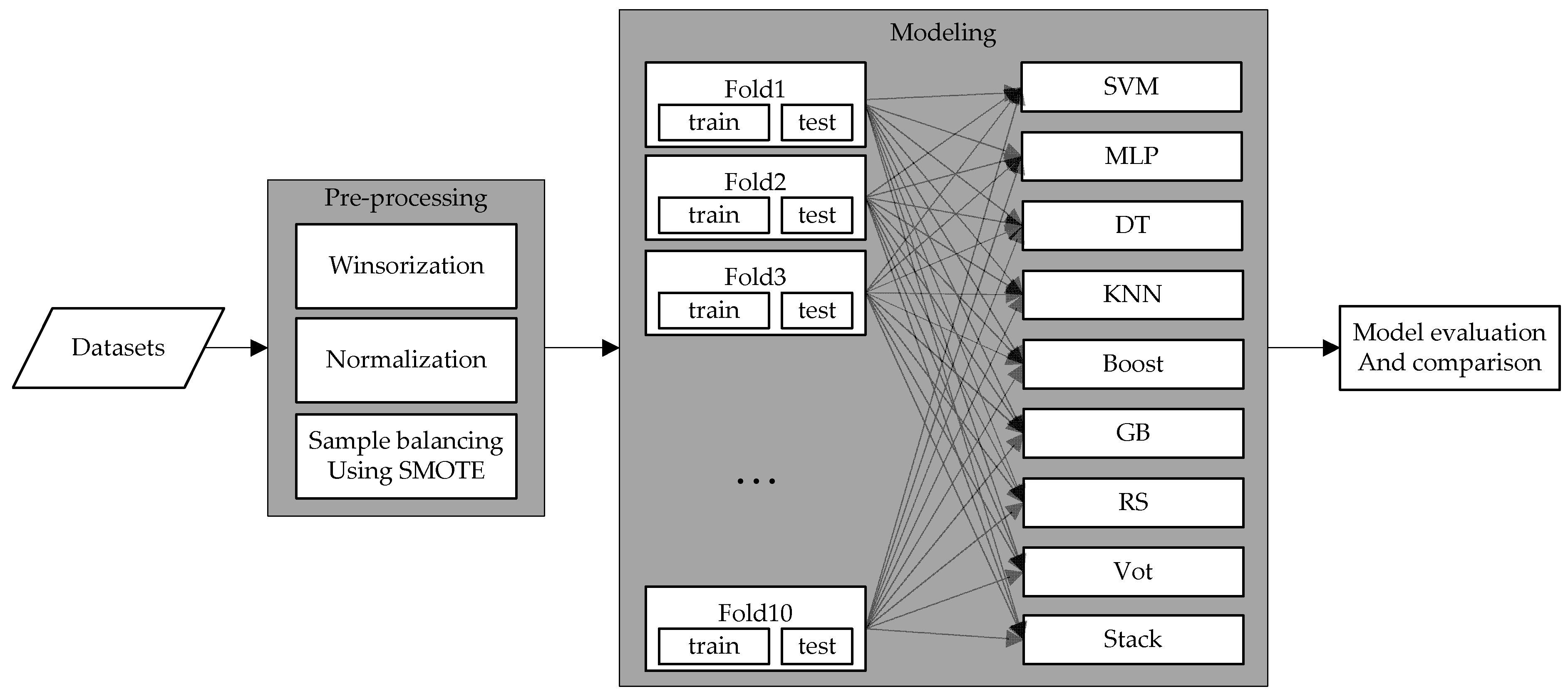
The experiments in this study used four single-machine learning models (SVM, MLP, DT, and KNN) and machine learning ensemble models (Boost, GB, RS, Vot, and Stack) to predict the medium-to-long-term financial distress of construction companies. The experiments in this study were carried out using the Python programming language [
60], and the Python scikit-learn library [
61] was used for data processing and implementing the machine learning models.
Figure 1 illustrates the entire framework of the experimental setup.
4.2. Results
In this section, the predictive performance of the machine learning model is measured, and the results of statistical tests are discussed.
4.2.1. Performance Measure
Previous studies have demonstrated that the receiver operating characteristic (ROC) curve can be an excellent tool for evaluating prediction models of financial status [
36,
62,
63,
64,
65]. In the ROC curve, the
x-axis is the false positive rate (FPR), and the
y-axis is the true positive rate (TPR) and is drawn while changing the classification threshold from a minimum to a maximum value. The AUC had a value between 0 and 1 in the area under the ROC curve, less than 0.5, indicating that the performance of the classifier is less than a random guess. If it is 0.7 or higher, it shows a predictive performance that can be classified [
66,
67]. All classification algorithms use AUC for binary classes (financial normal-0, financial distress-1).
Table 5 summarizes the AUC values of each model for predicting the financial distress of construction companies.
The RS algorithm achieved the best prediction performance, yielding a score of 0.7675 concerning the AUC metric, followed by Vot with a score of 0.7578. In addition to exhibiting the best performance for the overall average, the RS ensemble showed a high prediction performance for individual years, ranking first, second, and first for three, five, and seven years ahead of the prediction point, respectively. The RS ensemble generated significant results exceeding single-machine learning prediction models. Based on these results, we confirmed that the RS algorithm performs better than the other algorithms in predicting the medium-to-long-term financial distress of construction companies.
4.2.2. Statistical Significance Test
In this study, statistical tests were used to determine significant differences in the ranking of prediction model performance. The Friedman test analyzes classification algorithms based on the ranking for each dataset [
68], and previous studies have compared the performance of the model. Comparing model performance using the average is not objective, considering that specific model performance is excessively high for one data fold. The Friedman test indicates that the ranking of multiple algorithms by comprehensively considering the performances derived from multiple folds can be evaluated, and the following hypothesis is proposed. The null hypothesis (H0) of the Friedman rank test indicates no difference in the performance of the predictive models.
Conversely, the alternative hypothesis (H1) indicates that at least one prediction model exhibits a significantly different performance than the other classifiers [
69]. This test examined the differences in the performance of the prediction models through significance testing.
Table 6 summarizes the Friedman rank test results for each model to predict the financial distress of construction companies.
The results from the Friedman rank test in terms of AUC presented a test statistic (value) of , which was smaller than the high significance level (α < 0.01). Based on this statistical test, the Friedman rank test null hypothesis (H0) is rejected, whereas the alternative hypothesis (H1) is accepted. Therefore, considering the results for performance in terms of AUC, we concluded that at least one prediction model exhibits significantly different performance than the others.
The relative prediction ranking of the Friedman test showed a similar order as the ranking of the mean AUC. According to the results of the Friedman test, the RS algorithm is a high-performing algorithm in most data folds and ranks 1.60th out of the nine algorithms. From these results, it can be confirmed that the RS algorithm shows good overall performance in the medium-to-long term and after a specific year prediction.
4.3. Discussion
As mentioned above, this study compared the performance of single-machine learning and ensemble models in predicting the financial distress of construction companies after a medium-to-long-term period. It was determined that the RS ensemble model had the highest AUC in prediction after three and seven years ahead of the prediction point. This model also exhibited the best performance among various machine learning models in comprehensive medium-to-long-term prediction evaluations based on the Friedman test. The second-best prediction performance was exhibited by the Vot ensemble model, which exhibited satisfactory performance for predicting the financial distress of construction companies after three years in existing studies. The RS algorithm exhibited the best performance because the Vot and RS models indicated a difference in the composition of base learners used for the ensemble and feature selection processes, despite the same ensemble methods used in these models. Unlike the Vot model, the RS model established an ensemble model by generating tens to hundreds of base learners, exhibiting the highest data classification performance. Based on these results, the ensemble models exhibited outstanding performance in predicting the financial distress of construction companies after a medium-to-long-term period.
All ensemble models indicated an AUC value of 0.7 or higher in the overall medium-to-long-term prediction experiments. Some single-machine learning models indicated an AUC value of 0.7 or lower. Generally, a model shows predictability for a classification problem when the AUC value is 0.7 or higher [
66,
67]. The evaluation results based on AUC values indicated that ensemble models better predict construction companies’ financial distress after a medium-to-long-term period than single-machine learning models.
The optimization results of the voting and stacking ensemble showed that the base learner did not merely select a single classification model with high accuracy. Because the algorithm’s purpose was to increase the prediction performance by combining single classification models with low prediction performance, we assumed that combining a single classification model with high prediction performance would yield the best result. However, the optimization results confirmed that the DT model was selected as the base learner of the stacking ensemble even though it performed less favorably than the MLP in terms of prediction after five years, which implies that even a single classification model with low accuracy can correct the class “misclassified” by the ones with high accuracy. Therefore, when constructing an ensemble model, the maximum number of single prediction models must be considered and optimized to ensure that they complement each other, even if their accuracies are low.
The results of this study are similar to the results of machine learning model performance in various real-life applications of soft-computing studies. Oza and Tumer [
70] reported that ensemble models generally utilize all available classifier information and can provide more robust solutions than single-machine learning models. Li and Chen [
71] evaluated corporate credit based on an ensemble model and verified that it exhibited better evaluation performance than single-machine learning models. However, the boosting models did not perform better than the other ensemble models. These results reveal the importance of generalized learning ability for outliers, one of the main characteristics of financial data when predicting medium-to-long-term financial difficulties of construction companies, which is consistent with the results of previous studies [
71,
72].
5. Conclusions
In the implementation process of large construction projects, the financial distress of construction companies is a crucial issue that might affect project stakeholders, such as investors and subcontractors, and even has a national-level influence. Numerous studies have been performed to predict the financial status of companies in the construction industry; however, most of these studies focused on prediction a year after the prediction point. A few studies predicted the financial status of companies by considering only three years ahead of the prediction point. The average implementation period for large construction projects is 4.8 years, and a few large construction projects require a longer implementation period. In this regard, it can be concluded that predictions based on three years or less are insufficient to identify the financial status of companies in selecting a construction company that will be responsible for implementing a large-scale project. Thus, this study aims to propose suitable models for predicting the financial distress of construction companies for three-, five-, and seven-year periods through the use of variables affecting the company’s financial status after the medium-to-long-term period and to compare the performance of various prediction models.
The main contributions of this paper are as follows:
- (1)
The proposed prediction method can predict the financial status of construction companies based on three, five, and seven years ahead of the prediction point by considering the entire period of large-scale construction projects, which tend to be conducted for approximately five years on average, ranging from project planning to completion.
- (2)
To select input variables for the medium-to-long-term prediction model, this study utilized 17 financial indicators, which were applied multiple times in previous studies on medium-to-long-term prediction in other industries and were verified to affect the financial status of companies after the period.
- (3)
By comparing the performance of a single-machine learning model and an ensemble model, this study demonstrated that the ensemble model generally performs well in medium-to-long-term predictions.
This study compared the performance of prediction models using data on the financial status of construction companies in Korea collected from 2009 to 2018. The comparison result of the RS model exhibited high performance in predicting financial distress for three, five, and seven years ahead of the prediction point. The results of the Friedman test also revealed that the RS model was ranked highest for relative prediction performance among the nine models and that this model exhibited the best performance for comprehensive medium-to-long-term predictions. These analytical results indicate that the RS model can provide more accurate information on companies than other prediction models in evaluating the financial status of construction companies after a medium-to-long-term period. Consequently, this study proposes an algorithm that generally exhibits excellent performance. The proposed algorithm can be effectively employed to help large-scale project stakeholders evaluate the financial status of construction companies after a medium-to-long-term period during the project planning stage.
Despite the results above, this study had several limitations. This study adopted a financial ratio, which has been applied in previous studies to predict the financial status of companies after a medium-to-long-term period, as an input variable. However, external factors other than the financial ratio can affect companies’ financial status. Thus, in addition to corporate financial data, it is necessary to consider the use of other construction project indicators, stocks, and macroeconomics and to analyze the sensitivity of added variables to identify those having a major impact on the medium-to-long-term financial distress of construction companies. Moreover, this study used financial data obtained at a certain point instead of other data types, such as sequential and spatial data. Accordingly, this study failed to compare the prediction results with those based on the deep learning technique. In the future, studies should compare predictive performance with more diverse deep learning and hybrid models and consider using various data such as time series and matrix types. Finally, in addition to Bayesian optimization, there is an urgency to shorten the learning optimization time of the model and improve the prediction performance using hyperparameter optimization techniques such as genetic algorithms.
Author Contributions
Conceptualization, J.J. and C.K.; Data curation, J.J. and C.K.; Formal analysis, J.J.; Funding acquisition, C.K.; Investigation, J.J. and C.K.; Methodology, J.J. and C.K.; Project administration, C.K.; Resources, J.J. and C.K.; Software, J.J.; Supervision, C.K.; Validation, J.J. and C.K.; Visualization, J.J.; Writing—original draft, J.J. and C.K.; Writing—review and editing, C.K. All authors have read and agreed to the published version of the manuscript.
Funding
This study was supported by the Basic Science Research Program through the National Research Foundation of Korea, funded by the Ministry of Education (NRF-2018R1D1A1B07049846) and the Chung-Ang University Graduate Research Scholarship (GRS) in 2020.
Conflicts of Interest
The authors declare no conflict of interest.
References
- Flyvbjerg, B. What you should know about megaprojects and why: An overview. Proj. Manag. J. 2014, 45, 6–19. [Google Scholar] [CrossRef] [Green Version]
- Conway, H.M.; Lyne, L. Global Super Projects: Mega Ventures Shaping our Future; Conway Data: Peachtree Corners, GA, USA, 2006. [Google Scholar]
- Winch, G.M. Industrial megaprojects: Concepts, strategies, and practices for success. Constr. Manag. Econ. 2012, 30, 705–708. [Google Scholar] [CrossRef]
- Yi, H.; Chan, A.P.; Yun, L.; Jin, R.Z. From Construction Megaproject Management to Complex Project Management: Bibliographic Analysis. J. Manag. Eng. 2015, 31, 04014052. [Google Scholar]
- Zou, P.X.; Zhang, G.; Wang, J. Understanding the key risks in construction projects in China. Int. J. Proj. Manag. 2007, 25, 601–614. [Google Scholar] [CrossRef]
- Xu, X.; Wang, J.; Li, C.Z.; Huang, W.; Xia, N. Schedule risk analysis of infrastructure projects: A hybrid dynamic approach. Autom. Constr. 2018, 95, 20–34. [Google Scholar] [CrossRef]
- Jahren, C.T.; Ashe, A.M. Predictors of cost-overrun rates. J. Constr. Eng. Manag. 1990, 116, 548–552. [Google Scholar] [CrossRef]
- Love, P.E.; Zhou, J.; Edwards, D.J.; Irani, Z.; Sing, C.P. Off the rails: The cost performance of infrastructure rail projects. Transp. Res. Part A Policy Pract. 2017, 99, 14–29. [Google Scholar] [CrossRef]
- Heravi, G.; Mohammadian, M. Investigating cost overruns and delay in urban construction projects in Iran. Int. J. Constr. Manag. 2021, 21, 958–968. [Google Scholar] [CrossRef]
- Long, N.D.; Ogunlana, S.; Quang, T.; Lam, K.C. Large construction projects in developing countries: A case study from Vietnam. Int. J. Proj. Manag. 2004, 22, 553–561. [Google Scholar] [CrossRef]
- Pinheiro Catalão, F.; Cruz, C.O.; Miranda Sarmento, J. Exogenous determinants of cost deviations and overruns in local infrastructure projects. Constr. Manag. Econ. 2019, 37, 697–711. [Google Scholar] [CrossRef]
- Le-Hoai, L.; Lee, Y.D.; Lee, J.Y. Delay and cost overruns in Vietnam large construction projects: A comparison with other selected countries. KSCE J. Civ. Eng. 2008, 12, 367–377. [Google Scholar] [CrossRef]
- Toor, S.U.R.; Ogunlana, S.O. Problems causing delays in major construction projects in Thailand. Constr. Manag. Econ. 2008, 26, 395–408. [Google Scholar] [CrossRef]
- Zidane, Y.J.-T.; Andersen, B. The top 10 universal delay factors in construction projects. Int. J. Manag. Proj. Bus. 2018, 11, 650–672. [Google Scholar] [CrossRef]
- Hussain, S.; Zhu, F.; Ali, Z.; Aslam, H.D.; Hussain, A. Critical delaying factors: Public sector building projects in Gilgit-Baltistan, Pakistan. Buildings 2018, 8, 6. [Google Scholar] [CrossRef] [Green Version]
- Huang, H.-T.; Tserng, H.P. A study of integrating support-vector-machine (SVM) model and market-based model in predicting Taiwan construction contractor default. KSCE J. Civ. Eng. 2018, 22, 4750–4759. [Google Scholar] [CrossRef]
- KISVALUE, NICE Information Service. Available online: https://www.kisvalue.com/web/index.jsp (accessed on 15 January 2022).
- Chen, W.H.; Shih, J.Y. A study of Taiwan’s issuer credit rating systems using support vector machines. Expert Syst. Appl. 2006, 30, 427–435. [Google Scholar] [CrossRef]
- Qing, L. Credit Rating and Real Estate Investment Tust. Ph.D. Thesis, Nankai University, Nankai, China, 2014. [Google Scholar]
- eCREDIT, NICE Information Service. Available online: https://www.ecredit.co.kr/rq/RQ0100M000GE.nice (accessed on 24 September 2022).
- Morningstar Credit Ratings, Definitions and Other Related Opinions and Identifiers. Available online: https://ratingagency.morningstar.com/PublicDocDisplay.aspx?i=%2b7cwsQ2XW8A%3d&m=i0Pyc%2bx7qZZ4%2bsXnymazBA%3d%3d&s=LviRtUKXqs8kml5dHt7FTeE2SZmY0Fvqd4iX49Mk%2f9UapyiFTEO6TA%3d%3d (accessed on 17 September 2022).
- Horta, I.M.; Camanho, A.S. Company failure prediction in the construction industry. Expert Syst. Appl. 2013, 40, 6253–6257. [Google Scholar] [CrossRef]
- Ng, S.T.; Wong, J.M.; Zhang, J. Applying Z-score model to distinguish insolvent construction companies in China. Habitat Int. 2011, 35, 599–607. [Google Scholar]
- Adeleye, T.; Huang, M.; Huang, Z.; Sun, L. Predicting loss for large construction companies. J. Constr. Eng. Manag. 2013, 139, 1224–1236. [Google Scholar] [CrossRef]
- Heo, J.; Yang, J.Y. AdaBoost based bankruptcy forecasting of Korean construction companies. Appl. Soft Comput. 2014, 24, 494–499. [Google Scholar] [CrossRef]
- Choi, H.; Son, H.; Kim, C. Predicting financial distress of contractors in the construction industry using ensemble learning. Expert Syst. Appl. 2018, 110, 1–10. [Google Scholar] [CrossRef]
- Kangari, R.; Farid, F.; Elgharib, H.M. Financial performance analysis for construction industry. J. Constr. Eng. Manag. 1992, 118, 349–361. [Google Scholar] [CrossRef]
- Cheng, M.-Y.; Hoang, N.-D. Evaluating contractor financial status using a hybrid fuzzy instance based classifier: Case study in the construction industry. IEEE Trans. Eng. Manag. 2015, 62, 184–192. [Google Scholar] [CrossRef]
- Tserng, H.P.; Chen, P.-C.; Huang, W.-H.; Lei, M.C.; Tran, Q.H. Prediction of default probability for construction firms using the logit model. J. Civ. Eng. Manag. 2014, 20, 247–255. [Google Scholar] [CrossRef] [Green Version]
- International Contractors Association of Korea, Average Construction Period. Available online: http://kor.icak.or.kr/ (accessed on 11 February 2022).
- Li, H.; Sun, J. Predicting business failure using multiple case-based reasoning combined with support vector machine. Expert Syst. Appl. 2009, 36, 10085–10096. [Google Scholar] [CrossRef]
- Wang, L.; Wu, C. A combination of models for financial crisis prediction: Integrating probabilistic neural network with back-propagation based on adaptive boosting. Int. J. Comput. Intell. Syst. 2017, 10, 507–520. [Google Scholar] [CrossRef] [Green Version]
- Zhang, Y.; Wang, S.; Ji, G. A rule-based model for bankruptcy prediction based on an improved genetic ant colony algorithm. Math. Probl. Eng. 2013, 2013, 753251. [Google Scholar] [CrossRef]
- Geng, R.; Bose, I.; Chen, X. Prediction of financial distress: An empirical study of listed Chinese companies using data mining. Eur. J. Oper. Res. 2015, 241, 236–247. [Google Scholar] [CrossRef]
- Ding, Y.; Song, X.; Zen, Y. Forecasting financial condition of Chinese listed companies based on support vector machine. Expert Syst. Appl. 2008, 34, 3081–3089. [Google Scholar] [CrossRef]
- Du Jardin, P. Dynamics of firm financial evolution and bankruptcy prediction. Expert Syst. Appl. 2017, 75, 25–43. [Google Scholar] [CrossRef]
- Scacun, N.; Voronova, I. Evaluation of enterprise survival: Case of Latvian enterprises. Bus. Manag. Econ. Eng. 2018, 16, 13–26. [Google Scholar] [CrossRef]
- Wang, G.; Chen, G.; Chu, Y. A new random subspace method incorporating sentiment and textual information for financial distress prediction. Electron. Commer. Res. Appl. 2018, 29, 30–49. [Google Scholar] [CrossRef]
- Jones, S.; Wang, T. Predicting private company failure: A multi-class analysis. J. Int. Financ. Mark. Inst. Money 2019, 61, 161–188. [Google Scholar] [CrossRef]
- Mai, F.; Tian, S.; Lee, C.; Ma, L. Deep learning models for bankruptcy prediction using textual disclosures. Eur. J. Oper. Res. 2019, 274, 743–758. [Google Scholar] [CrossRef]
- Song, Y.; Peng, Y. A MCDM-based evaluation approach for imbalanced classification methods in financial risk prediction. IEEE Access 2019, 7, 84897–84906. [Google Scholar] [CrossRef]
- Altman, E.I.; Iwanicz-Drozdowska, M.; Laitinen, E.K.; Suvas, A. A race for long horizon bankruptcy prediction. Appl. Econ. 2020, 52, 4092–4111. [Google Scholar] [CrossRef]
- Korol, T. Long-term risk class migrations of non-bankrupt and bankrupt enterprises. J. Bus. Econ. Manag. 2020, 21, 783–804. [Google Scholar] [CrossRef]
- Rose, P.S.; Giroux, G.A. Predicting corporate bankruptcy: An analytical and empirical evaluation. Rev. Financ. Econ. 1984, 19, 1. [Google Scholar]
- Zarb, B.J. Earning power and financial health in the airline industry-a preliminary investigation of US and non-US airlines. Int. J. Bus. Acc. Financ. 2010, 4, 119–133. [Google Scholar]
- Karas, M.; Reznakova, M. Identification of financial signs of bankruptcy: A case of industrial enterprises in the Czech Republic. In Proceedings of the 6th International Scientific Conference: Finance and the Performance of Firms in Science, Education, and Practise, Zlin, Czech Republic, 25–26 April 2013; pp. 324–335. [Google Scholar]
- Thammasiri, D.; Delen, D.; Meesad, P.; Kasap, N. A critical assessment of imbalanced class distribution problem: The case of predicting freshmen student attrition. Expert Syst. Appl. 2014, 41, 321–330. [Google Scholar] [CrossRef] [Green Version]
- Chawla, N.V.; Bowyer, K.W.; Hall, L.O.; Kegelmeyer, W.P. SMOTE: Synthetic minority over-sampling technique. J. Artif. Intell. Res. 2002, 16, 321–357. [Google Scholar] [CrossRef]
- Xie, W.; Liang, G.; Dong, Z.; Tan, B.; Zhang, B. An improved oversampling algorithm based on the samples’ selection strategy for classifying imbalanced data. Math. Probl. Eng. 2019, 2019, 3526539. [Google Scholar] [CrossRef]
- Hsu, C.-W.; Lin, C.-J. A comparison of methods for multiclass support vector machines. IEEE Trans. Neural Netw. 2002, 13, 415–425. [Google Scholar]
- Sinha, P.; Sinha, P. Comparative study of chronic kidney disease prediction using KNN and SVM. J. Eng. Res. Technol. 2015, 4, 608–612. [Google Scholar]
- Bedi, J.; Toshniwal, D. Deep learning framework to forecast electricity demand. Appl. Energy 2019, 238, 1312–1326. [Google Scholar] [CrossRef]
- Bergstra, J.; Yamins, D.; Cox, D. Making a science of model search: Hyperparameter optimization in hundreds of dimensions for vision architectures. In Proceedings of the International conference on machine learning, Atlanta, GA, USA, 16–21 June 2013; pp. 115–123. [Google Scholar]
- Zhang, W.; Wu, C.; Zhong, H.; Li, Y.; Wang, L. Prediction of undrained shear strength using extreme gradient boosting and random forest based on Bayesian optimization. Geosci. Front. 2021, 12, 469–477. [Google Scholar] [CrossRef]
- Nyitrai, T.; Virág, M. The effects of handling outliers on the performance of bankruptcy prediction models. Socio-Econ. Plan. Sci. 2019, 67, 34–42. [Google Scholar] [CrossRef]
- Tian, S.; Yu, Y. Financial ratios and bankruptcy predictions: An international evidence. Int. Rev. Econ. Financ. 2017, 51, 510–526. [Google Scholar] [CrossRef]
- Xu, W.; Fu, H.; Pan, Y. A novel soft ensemble model for financial distress prediction with different sample sizes. Math. Probl. Eng. 2019, 2019, 3085247. [Google Scholar] [CrossRef] [Green Version]
- Kohavi, R. A study of cross-validation and bootstrap for accuracy estimation and model selection. Ijcai 1995, 14, 1137–1145. [Google Scholar]
- Son, H.; Kim, C.; Hwang, N.; Kim, C.; Kang, Y.J.A.E.I. Classification of major construction materials in construction environments using ensemble classifiers. Adv. Eng. Inform. 2014, 28, 1–10. [Google Scholar] [CrossRef]
- RRossum, G. Python Reference Manual. Available online: http://www.python.org/ (accessed on 19 May 2022).
- Pedregosa, F.; Varoquaux, G.; Gramfort, A.; Michel, V.; Thirion, B.; Grisel, O.; Blondel, M.; Prettenhofer, P.; Weiss, R.; Dubourg, V.; et al. Scikit-learn: Machine learning in Python. J. Mach. Learn. Res. 2011, 12, 2825–2830. [Google Scholar]
- Sobehart, J.R.; Keenan, S.C.; Stein, R.M. Benchmarking Quantitative Default Risk Models: A Validation Methodology; Moody’s InvestorsService: New York, NY, USA, 2000; Available online: http://www.rogermstein.com/wp-content/uploads/53621.pdf (accessed on 10 June 2022).
- Stein, R.M. Benchmarking default prediction models: Pitfalls and remedies in model validation. J. Risk Model Valid. 2002, 1, 77–113. [Google Scholar] [CrossRef] [Green Version]
- Agarwal, V.; Taffler, R. Comparing the performance of market-based and accounting-based bankruptcy prediction models. J. Bank. Financ. 2008, 32, 1541–1551. [Google Scholar] [CrossRef] [Green Version]
- Tserng, H.P.; Liao, H.-H.; Tsai, L.K.; Chen, P.-C. Predicting construction contractor default with option-based credit models—Models’ performance and comparison with financial ratio models. J. Constr. Eng. Manag. 2011, 137, 412–420. [Google Scholar] [CrossRef]
- Mandrekar, J.N. Receiver operating characteristic curve in diagnostic test assessment. J. Thorac. Oncol. 2010, 5, 1315–1316. [Google Scholar] [CrossRef] [Green Version]
- Hosmer, D.W., Jr.; Lemeshow, S.; Sturdivant, R.X. Applied Logistic Regression; John Wiley & Sons: Hoboken, NJ, USA, 2013; Volume 398. [Google Scholar]
- Grinberg, N.F.; Orhobor, O.I.; King, R.D. An evaluation of machine-learning for predicting phenotype: Studies in yeast, rice, and wheat. Mach. Learn. 2020, 109, 251–277. [Google Scholar] [CrossRef] [Green Version]
- Verma, A.; Ranga, V. Machine learning based intrusion detection systems for IoT applications. Wirel. Pers. Commun. 2020, 111, 2287–2310. [Google Scholar] [CrossRef]
- Oza, N.C.; Tumer, K. Classifier ensembles: Select real-world applications. Inf. Fusion 2008, 9, 4–20. [Google Scholar] [CrossRef]
- Li, Y.; Chen, W. A comparative performance assessment of ensemble learning for credit scoring. Mathematics 2020, 8, 1756. [Google Scholar] [CrossRef]
- Freund, Y.; Schapire, R.E. Experiments with a new boosting algorithm. In Proceedings of the Thirteenth International Conference on International Conference on Machine Learning, Bari, Italy, 3–6 July 1996; Morgan Kaufmann Publishers: Burlington, MA, USA, 1996; pp. 148–156. [Google Scholar]
| Publisher’s Note: MDPI stays neutral with regard to jurisdictional claims in published maps and institutional affiliations. |
© 2022 by the authors. Licensee MDPI, Basel, Switzerland. This article is an open access article distributed under the terms and conditions of the Creative Commons Attribution (CC BY) license (https://creativecommons.org/licenses/by/4.0/).


