Nonlinear Modeling of RC Substandard Beam–Column Joints for Building Response Analysis in Support of Seismic Risk Assessment and Loss Estimation

Abstract

The paper discusses how joint damage and deterioration affect the seismic response of existing reinforced concrete frames with sub-standard beam–column joints. The available simplified modeling techniques are critically reviewed to propose a robust, yet computationally efficient, technique for simulating the nonlinear behavior of substandard beam–column joints. Improvements over the existing models include the simulation of the cyclic deterioration of joint stiffness and strength, as well as pinching in the hysteretic response, implemented considering a deteriorating hysteretic rule. A fiber-section forced-based inelastic beam–column element is developed, considering improved material models and fixed-end rotation due to bond failure, rebars-slip, and inelastic extension, to simulate the deteriorating cyclic behavior of existing pre-cracked beam–column members. For the assessment of frames with substandard exterior beam–column joints, a nonlinear model for the exterior joint is developed and validated through a full-scale quasi-static cyclic test performed on a substandard T-joint connection. The proposed model allows considering structural performance in risk assessment while accounting for true inelastic mechanisms at the joints. An assessment of a five-story RC frame revealed that the activation of the joint shear mechanism increases the chord rotation demand on the connecting beam members by up to 85%, with increases of up to 62% (mean drift) and 89% (mean + 1.std.) on the lower floors when determining the inter-story drift demand, and the collapse probability of structures subjected to design base ground motions increased from 4.20% to 29.20%.

1. Introduction

A beam–column joint in a reinforced concrete moment-resisting frame is a most critical component; it experiences high axial and vertical/horizontal shear stresses during earthquakes, and its behavior has a significant influence on the building seismic response. If not adequate, joint shear failure can result. However, if a joint is assumed to be stiff throughout the analysis during the assessment process, this may be overlooked. The shear failure of the beam–column joint often has a brittle character, which does not provide an adequate level of structural performance, particularly under extreme seismic actions [1,2]. There have been several reports of catastrophic building collapses during strong earthquakes (Figure 1), which have been linked to beam–column joint failure, including those that occurred in the 1999 earthquakes in Chi-Chi, Taiwan, and Izmit, Turkey, and in the 1994 Northridge earthquake in California, USA [3]. Therefore, it is crucial to comprehend joint behavior in nonlinear building response analysis in order to make an informed judgment regarding the evaluation of building damages.

Over the past several decades, a number of studies have focused on understanding how beam–column joints respond to seismic actions [4,5,6,7,8,9,10,11]. Moreover, several international seismic codes of practice have undergone repeated improvements to put the findings into practice. The most recent ACI joint design recommendations [12] account for inelastic deformation in the joint panel. The present joint design procedures and detailing provisions offer resistance to the gravity loads, seismic actions, and the interaction of multidirectional forces applied to the joint from surrounding frame elements. To ensure an improved cycle behavior and a minimum plastic deformation capacity, sufficient development length and confinement in the joint panel are provided.

Recent research on the quantification of the seismic risk of existing reinforced concrete structures has focused on frames with the substandard beam–column joints that are prevailing in most seismically active countries. This paper focuses on comprehending the primary mechanism influencing the seismic nonlinear response of beam–column connections and presents a simplified nonlinear numerical modeling technique, which is crucial for assessing the seismic building’s response. With particular reference to bond failure and rebar slip (resulting in member fixed-end rotation) and joint shear strength deterioration, this research studied the effects of exterior joint nonlinear behavior and underlines the crucial factors that influence structural performance, which is fundamental for risk assessment and repair cost estimation.

The experimental reference specimen of the exterior beam–column joint under consideration was designed in accordance with the previous building code of Pakistan but lacked seismic details and incorporated deficiencies prevalent in the typical beam–column joint in existing RC structures [13]. The test specimen was initially subjected to force-controlled cyclic loading in order to induce cracks in the specimen and simulate the pre-cracked condition of the current RC frame. The main finding is presented in terms of damage observations and the connection’s force–displacement hysteretic response to guide numerical modeling. The study is unique in that it takes into account pre-cracking in the substandard exterior beam–column joints that exhibit deterioration in the stiffness and strength of the connection.

2. Critical Review of Simplified Nonlinear Modeling Techniques for RC Beam–Column Joints

Modeling frames with weaker joints for nonlinear seismic analysis has been attempted using different simplified techniques (Figure 2). These are briefly reviewed here to serve as a basis for the development of a more robust, yet simplified and computationally efficient, analytical model of reinforced concrete frames that incorporates both shear and bond mechanisms behavior of beam–column joints and fixed-end rotation of connecting members due to pre-cracked beam–column members common to existing buildings and that can be used for both local and global damage evaluation to help guide retrofitting efforts.

The flexural strengths of the beams and columns framing the joint were decreased by Kunnath et al. [25] to take into consideration the insufficient joint shear strength capacity. However, such implicit models are incapable of accounting for the additional deformation resulting from the joint bond mechanism and the pinching effects on the frame hysteretic response due to joint shear stiffness and strength deterioration. Neverthless, the model is promising for the assessment of global performance. El-Metwally et al. [14] used a zero-length spring with nonlinear behavior to model the shear deformation of the joint panel. Through the use of rotational springs, Biddah and Ghobarah [16] modeled joint shear and bond-slip deformations. Later, Ghobarah and Biddah [26] utilized the model to demonstrate that joint deformations led to greater flexibility and drifts under seismic actions. The models were promising for frames with joints with stable behavior; however, these models were unable to accurately simulate the joint shear stiffness and strength deterioration essential for substandard joints. Alath and Kunnath [15] used a rotational spring model to explicitly simulate the joint shear deformation, with deteriorating hysteresis being established empirically, but this has the drawback that it must repeatedly be calibrated for various beam–column joints. Pampanin et al. [23] proposed a similar simplified model with a moment–rotational spring and deteriorating hysteretic response. The spring’s properties were directly deduced from the corresponding principal tensile stress vs. shear deformation curve, which, in turn, was based on a large experimental database [27], using the equilibrium consideration. This, however, falls short of accurately simulating the deterioration of joint shear strength. Sharma et al. [24] improved upon this approach by including additional shear springs in the joint panel to account for the panel’s shear deformation and to take strength degradation into consideration. The model still does not adequately account for stiffness and strength deterioration, i.e., cyclic deterioration (number-of-cycles effect), which is essential for substandard beam–column joints. The same is true for the method proposed by Khan et al. [28].

Adding an extra infinitely stiff bar attached to the plastic beam sub-element with plastic hinges at the ends, Filippou et al. [29] and Filippou and Issa [30] developed an explicit model to simulate the fixed-end rotations and the sliding due to shear at the beam–column interface. Although promising in simulating the rotational and bending-moment resistance of a beam–column joint, it is unable to simulate the joint shear deterioration and the pinching that results in the hysteretic response of the frame.

Youssef and Ghobarrah [18] developed a 14-spring element assembly for a beam–column joint that included two diagonal springs to simulate joint shear deformation and twelve translational springs placed at the panel zone interface to represent the inelastic mechanisms of connecting beam/column members. It models the shear strength deterioration but implicitly considers rebar slip and rebar inelasticity. A model developed by Ning et al. [21] included one spring for the panel zone and eight springs for the rebar-slip and employed the Bouc–Wen–Baber–Noori model [31] to simulate the hysteretic behavior of the panel zone. The model, however, is unable to truly replicate the cyclic strength and stiffness deterioration that often occurs at substandard beam–column joints.

Another model suggested by Elmorsi et al. [22] involved idealizing beams and columns as elastic elements connected to the joint by the intervention of non-linear transitional elements, modeled using other elements made up of 12 parts. The model takes into account the effects of bond-slip and joint shear deformations and can simulate the deterioration of bonds and eventual pullout of reinforcing bars during extreme cyclic loads. However, the model is clumsy and computationally expensive when a large number of analyses are required for building performance assessment.

A 4-node 12-degree-of-freedom joint panel was proposed by Lowes and Altoontash [17] that constitutes a panel zone component with a zero-length rotational spring simulating the shear deformation of the joint with four additional zero-length shear springs for simulating the interface–shear deformations. A total of eight zero-length translational springs were included to simulate the bar slip. The panel zone’s shear stress–strain relationships were determined using the modified compression field theory (MCFT) [32]. Later, Lowes et al. [33] attempted to simulate the interface-shear based on experimental data; this work anticipated an interface-shear response that was stiff and elastic. Moreover, specimens with at least a minimal degree of transverse reinforcement in the panel zone were included in the experimental data for validation, which is compatible with the model’s intended usage. However, they did not include joints that lack transverse reinforcement; therefore, it could not be used to analyze the weaker joints of frames that lack transverse reinforcement. The model proposed by Lowes and Altoontash [17] was further simplified by Altoontash [20] by adding four rotational springs to member ends to simulate the bar-slip phenomenon and a rotational spring that was defined in the panel zone to simulate the shear distortion of the joint. However, it is still insufficient for the analysis of joints lacking transverse reinforcement and members exhibiting large fixed-end rotation due to pre-cracked beam–column members.

Shin and LaFave [19] proposed an analytical model for a beam–column joint wherein the joint panel was made up of stiff elements along the panel zone’s edges and three parallel rotational springs provided in one of the four hinges connecting the parallelogram’s sides. The MCFT was used to anticipate the joint shear stress–strain response envelope while the cyclic response was calibrated using experimental data. Two rotating springs (in series) were positioned at the interfaces between the beam and the joint to separately simulate the member-end rotations produced by the bond-slip behavior of the longitudinal beam reinforcement and plastic hinge rotations induced by the inelastic behavior of the beam. The model is robust in simulating joint shear deterioration, bond mechanisms, and fixed-end rotation. However, the joint rotational springs needs simplification.

The assessment of beam–column joints without transverse reinforcement presents some difficulties for most of the modeling techniques discussed above. Some of these, for example, are computationally inefficient and need simplification in order to be implemented in the available finite element-based programs for large analysis, while others are only appropriate for joints that have been seismically designed and detailed and less accurate when applied to substandard beam–column joints with pre-existing cracks in the structural members. The goal of the present study is to propose a more robust modeling technique that would still be computationally efficient and capable of modeling the deterioration of stiffness and strength common to existing pre-cracked beam–column frames with substandard beam–column joints subjected to cyclic loading.

3. Proposed Nonlinear Modeling Technique for RC Substandard Beam–Column Joints

3.1. Mechanics of Exterior Beam–Column Joints

Figure 3 illustrates the internal forces and reactions acting on a reinforced concrete exterior beam–column joint under seismic actions. If it is assumed that the points of the zero bending moment are located at the half-height of the column and the half-span of the beam, respectively, then it can be assumed that column shear V_a = V_c and column moment M_a = M_c. The reversal of the moment across the joint necessitates that the reinforcement of the beam is in compression on one side and at a tensile yield on the other. The internal horizontal tension T_b, compression C_b, and vertical beam shear V_b forces introduced by the beam to the column are shown. Making the approximations that C_b = T_b, the required horizontal column shear force V_jh across the joint region based on the equilibrium of free body is:

$$V_{jh}=T_b-V_c$$

(1)

$$T_b=\frac{M_b}{j_b}$$

(2)

$$T_b=\frac{V_b{l}_b}{j_b}$$

(3)

where M_b is the beam moment, l_b is the length of beam, h_c is the depth of column, and j_b is the internal level arm between the tensile force and the centroid of the compressive forces. This can be determined by moment-curvature analysis of the beam or approximated as follows:

$$j_b=d_b-d_b^{\prime }$$

(4)

where d_b is the effective depth of beam and d′_b is the effective cover to compression reinforcement. The column top load V_c can be calculated corresponding to the beam moment extended linearly to the centerline of the joint:

$$V_c=\frac{V_b\left(l_b+0.5h_c\right)}{l_c}$$

(5)

where l_c is the length of column. Substituting Equations (5) and (3) in Equation (1), the following expression is obtained for horizontal joint shear force V_jh:

$$V_{jh}=V_b\left(\frac{l_b}{j_b}-\frac{l_b+0.5h_c}{l_c}\right)$$

(6)

The resulting horizontal and vertical shear stress, v_jh and v_jv, at the mid-depth of the joint core is:

$$v_{jh}=v_{jv}=\frac{V_{jh}}{h_c^{\prime }{b}_c^{\prime }}$$

(7)

where h′_c and b′_c are the length and width of joint core. The joint region is subjected to horizontal and vertical shear stresses that are typically many times greater than those in the adjacent beams and columns. However, the stresses are also dependent on the joint aspect ratio α:

$$\alpha =\frac{V_{jv}}{V_{jh}}=\frac{h_b}{h_c}$$

(8)

Moreover, the axial compressive stress f_a at the mid-depth of the joint core due to vertical force N_c acting on the column is:

$$f_a=\frac{N_c}{h_c^{\prime }{b}_c^{\prime }}$$

(9)

The joint shear and axial stresses lead to the diagonal compression and tension principal stresses in the joint core. The principal compression stress f_c and tension stress f_t at mid-depth of the joint core can be found using Mohr’s circle:

$$f_{t,c}=\frac{f_a}{2}\pm \sqrt{{\left(\frac{f_a}{2}\right)}^2+v_{jh}^2}$$

(10)

Once the joint core develops diagonal tension cracks, the joint core’s diagonal compression strut and truss mechanism, consisting of a concrete diagonal compression field and horizontal and vertical reinforcement, transfers the beam and column forces across the joint core (Figure 4). A beam-column joint may experience various damage or failure mechanisms as a result of the adopted structural detailing. It has been demonstrated that the use of poor-quality concrete, a lack of transverse reinforcement in the joint region, and inadequate anchoring details all constitute potential causes of a highly brittle failure mechanism. Because the shear and bond mechanisms that control the joint response have poor hysteretic properties, as a result, the joint’s rotational resistance degrades rapidly [34,35].

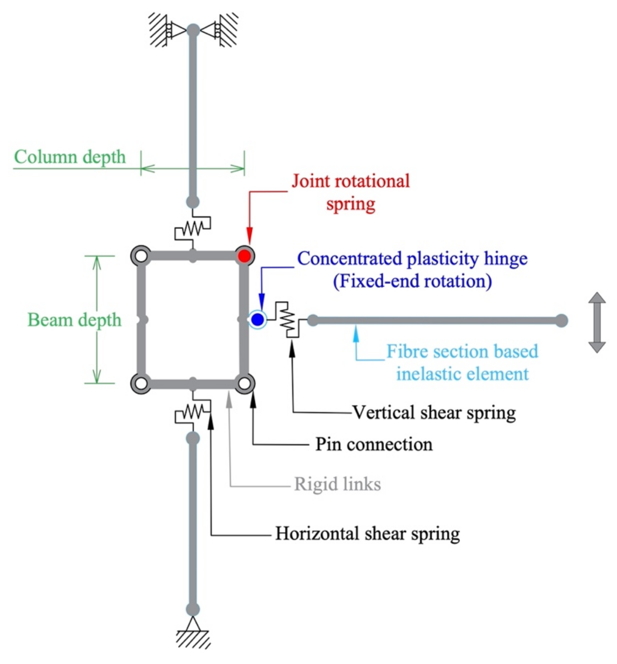
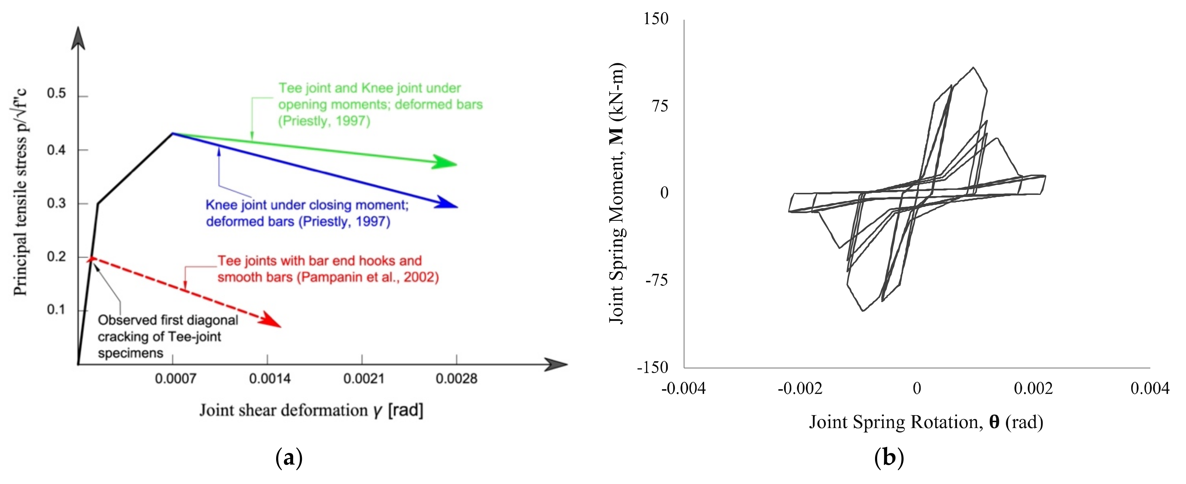
3.2. Modeling of Joint Shear Panel

Figure 5 illustrates the proposed analytical model for a substandard RC external beam–column joint subjected to seismic actions. A simplified flowchart is given in Appendix A (Figure A1) to help guide the preparation of a numerical model of structural systems. The beam elements and the column elements are located at the beam mid-depth and the column mid-depth, respectively. The assembly is envisaged, as the same is tested experimentally. The joint panel distortion is modeled by four rigid link elements arranged along the edges of the joint panel and one nonlinear rotational spring is incorporated in one of the four hinges connecting the adjacent rigid elements. The failure of an exterior joint is primarily related to the principal tensile stress developed in the joint core.

The critical parameter is the principal tension stress within the joint core, and joint cracking begins at a stress of 0.29 (f_c′)^0.5 MPa. In the case of exterior joints lacking transverse reinforcement, the experimental data support the highest principal tension stress of 0.42 (f_c′)^0.5. Joint shear strength deterioration is governed by the gradual reduction of the effective joint principal tension stress [27,36]. The principal tensile stress vs. shear deformation envelope curve illustrated in Figure 6a is used to directly deduce the moment–rotation properties of the joint spring based on the equilibrium considerations. The nonlinear rotational spring at the joint is assigned a multilinear deteriorating hysteretic rule [37] to simulate the joint stiffness and strength deterioration and pinching in the hysteretic response (Figure 6b), which is crucial for the shear failure of substandard beam–column joints.

The joint shear strength in the present model is only dependent on the concrete compressive strength, with no regard for the influence of additional factors such as the joint aspect ratio or longitudinal reinforcement of connecting elements. Although more contemporary shear strength models [10,38,39] can be used, the considered model is simple, requires less input information, and provides conservative estimates, which is useful for assessing existing RC frames.

3.3. Modeling of Beam–Column Connecting Members

The flexibility-based element formulation, such as that developed by Spacone et al. [40], which is an extension of the Ciampi and Carlesimo [41]-proposed consistent flexibility-based method for formulating frame members, is established using the framework of the mixed method formulation [42]. The element formulation strictly satisfies the equilibrium of bending moments and axial force along the element using force interpolation functions rather than displacement interpolation functions. The element state determination relies on a nonlinear iterative method based on residual deformations [42] that continuously maintain equilibrium within the element and finally converge to a state that satisfies the element constitutive relation within a set tolerance.

The element stiffness matrix is obtained by inverting the element flexibility matrix. The use of improved material models to simulate the element’s deteriorating hysteretic response owing to pre-existing cracks in the member, the rigid body fixed-end rotation due to rebars slip and inelastic extension, and geometric nonlinearity are improvements in the present model over the original formulation of Spacone et al. [40]. This solution technique is especially well suited for the study of the highly nonlinear deteriorating hysteretic behavior of the substandard reinforced concrete elements.

The fiber-based approach, in which each fiber is assigned a uniaxial stress–strain relationship, is used by the frame beam–column element to simulate the cross-section behavior. The nonlinear uniaxial stress–strain response of the individual fibers into which the section has been divided is then integrated to provide the sectional stress–strain state. Because the material constitutive models already specify hysteretic response, a fiber section-based element has the advantage of not requiring prior moment-curvature analysis and calibration. Moreover, it directly simulates the stiffness and strength interactions between an axial load and a bending moment, as well as the interactions between flexural strength in orthogonal directions. The discrete number of the controlling sections along the element that are used for the numerical integration is the only approximation in this formulation, and it does not actually impose any restrictions on the displacement field of the element, this formulation is always “exact”: regardless of the degree of inelasticity, the force field is always exact. To prevent under-integration, a minimum of 3 Gauss–Lobatto integration sections are necessary and in general 5–7 integration points (IPs) are utilized [43,44] to adequately model the spread of inelasticity.

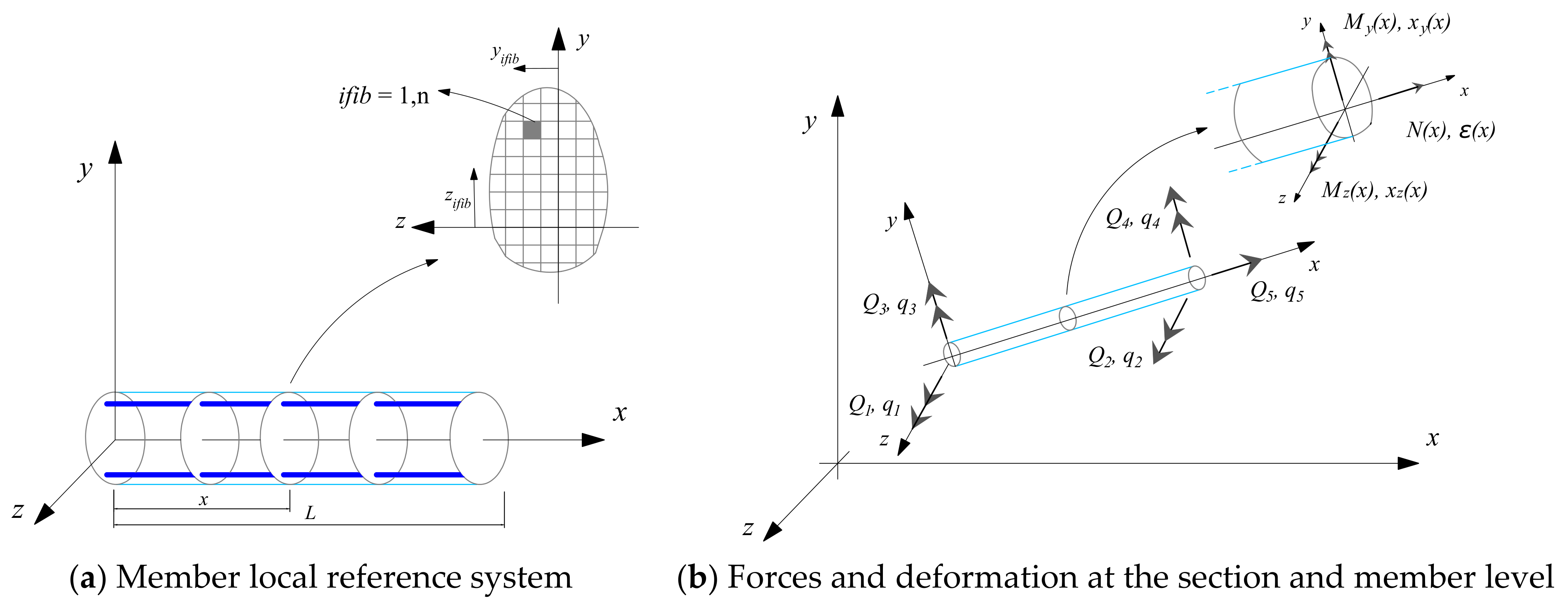
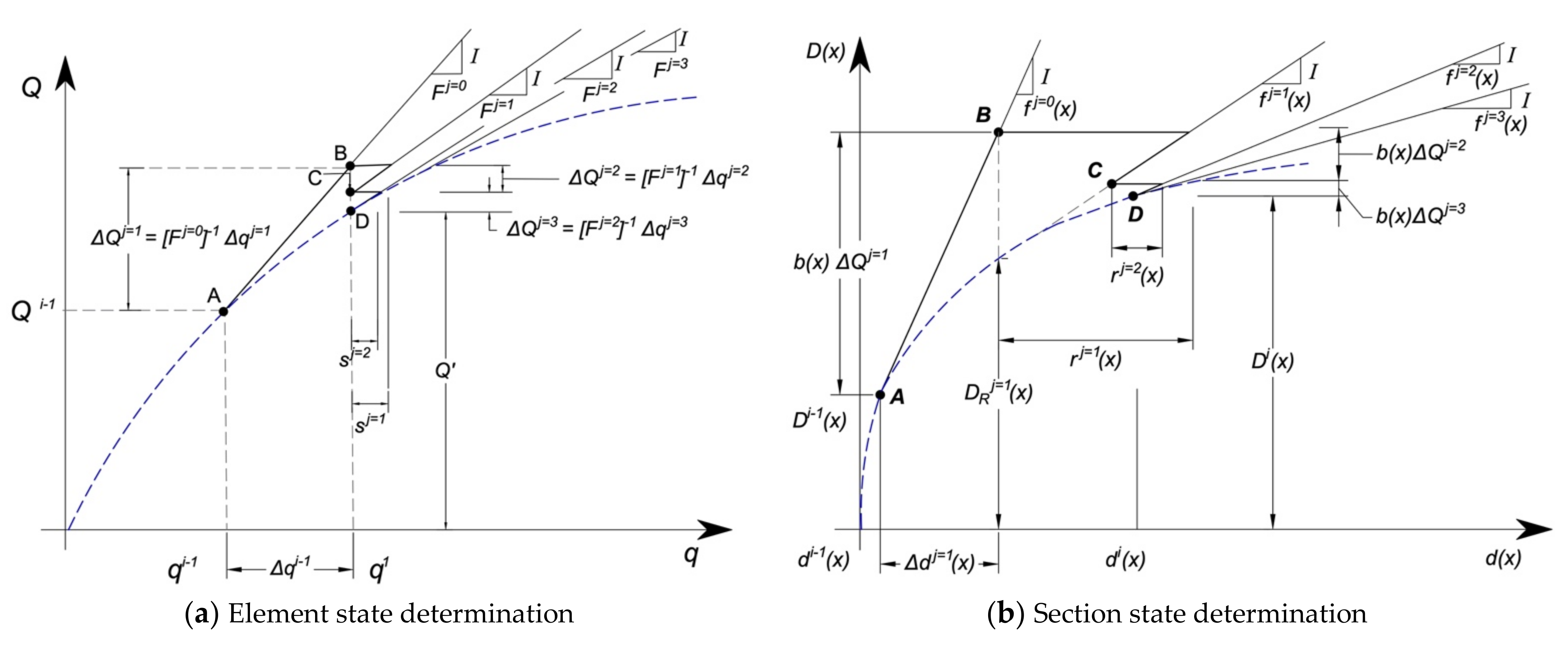
3.3.1. Beam–Column Element Formulation

Model assumptions:

• Beam–column element in local reference system x, y, z (Figure 7a)
• A discrete number of cross sections placed at control points of the numerical integration
• Beam–column member geometry is linear.
• Plane sections remain plane and are normal to the longitudinal axis throughout the deformation history.
• Strains and stresses act parallel to the longitudinal axis.
• Member behavior in torsion is linearly elastic and uncoupled from flexure and axial response.

Vectors of element forces and deformations and the corresponding section forces and deformations are given below:

$$Q={\left\{Q_1,Q_2,Q_3,Q_4\right\}}^T$$

(11)

$$q={\left\{q_1,q_2,q_3,q_4\right\}}^T$$

(12)

$$D\left(x\right)={\left\{M_z\left(x\right),M_y\left(x\right),N\left(x\right)\right\}}^T$$

(13)

$$d\left(x\right)={\left\{X_z\left(x\right),X_y\left(x\right),\overline{\epsilon }\left(x\right)\right\}}^T$$

(14)

where Q is the element force vector, q is the element deformation vector, D(x) is the section force vector, d(x) is the section deformation vector, X(x) is the section curvature about the reference axis, and $\overline{\epsilon }\left(x\right)$ is the axial strain at the reference axis. With the use of a simple geometric transformation matrix, the fiber strains are related to section deformations. The section forces and deformations are related to element forces and deformations using the force and deformation interpolation functions:

$$∆d\left(x\right)=a\left(x\right)∆q$$

(15)

$$∆D\left(x\right)=b\left(x\right)∆Q$$

(16)

where matrix a(x) is the deformation interpolation function, matrix b(x) is the force interpolation function, and Δ is the increments of the corresponding quantities. The linearization of the incremental section constitutive relation is according to the Equation (17):

$$∆d^j\left(x\right)=f^{j-1}\left(x\right)∆D^j\left(x\right)+r^{j-1}\left(x\right)$$

(17)

where $f^{j-1}\left(x\right)$ is the section flexibility and $r^{j-1}\left(x\right)$ is the residual deformations from the previous iteration. The residual deformation $r^{j-1}\left(x\right)$ is the linear approximation to the deformation error that results from linearizing the section force-deformation relation. Equation (17) may be presented in the integral form as given:

$${{\displaystyle \int }}_0^L\delta D^T\left(x\right)\left[∆d^j\left(x\right)-f^{j-1}\left(x\right)∆D^j\left(x\right)-r^{j-1}\left(x\right)\right]d_x=0$$

(18)

Substituting Equations (15) and (16) in Equation (18) gives:

$$T∆q^j-F^{j-1}∆Q^j-s^{j-1}=0.$$

(19)

where T is the matrix dependent on the interpolation functions, F is the element flexibility matrix, and s is the element residual deformation vector given as follows:

$$T={{\displaystyle \int }}_0^L{b}^T\left(x\right)a\left(x\right)d_x$$

(20)

$$F={{\displaystyle \int }}_0^L{b}^T\left(x\right)f\left(x\right)b\left(x\right)d_x$$

(21)

$$s={{\displaystyle \int }}_0^L{b}^T\left(x\right)r\left(x\right)d_x$$

(22)

Furthermore, the virtual displacement principle is used to obtain the integral form of the equilibrium equation:

$${{\displaystyle \int }}_0^L\delta d^T\left(x\right)\left[D^{j-1}\left(x\right)+∆D^j\left(x\right)\right]d_x=\delta q^T{Q}^j$$

(23)

where D^j−1(x) + D^j is the new internal force distribution and Q^j is the corresponding vector of nodal forces in equilibrium. Substituting Equations (15) and (16) in Equation (23), results in the following matrix expression, which is equivalent of the integral form of the element equilibrium equations:

$$T^T{Q}^{j-1}+T^T∆Q^j=Q^j$$

(24)

The combination of Equations (19) and (24) results in the following expression:

$$\left[\begin{array}{c}-F^{j-1} T\\ T^T 0\end{array}\right]=\left\{\begin{array}{c}∆Q^j\\ ∆q^j\end{array}\right\}=\left\{\begin{array}{c}{s}^{j-1}\\ Q^j-T^T{Q}^{j-1}\end{array}\right\}$$

(25)

Solving the first equation for ΔQ^j and substituting it in the second equation results in the following expression:

$$T^T{\left[F^{j-1}\right]}^{-1}\left(T∆q^j-s^{j-1}\right)=Q^j-T^T{Q}^{j-1}$$

(26)

Assuming T = I, as peculiar to the proposed Bernoulli beam, where I is a 3 × 3 identity matrix, the above equation is simplified as:

$${\left[F^{j-1}\right]}^{-1}\left(∆q^j-s^{j-1}\right)=∆Q^j$$

(27)

where ΔQ^j is the element force increment, (Δq^j − s^j−1) is the corresponding deformation increment including the residual deformation s^j−1 that results from the linearization of the section’s non-linear constitutive relations, and [F^j−1]⁻¹ is the element stiffness matrix obtained by inverting the flexibility matrix.

The element forces provide the most difficulty since they cannot be easily calculated from the section forces, even if the element stiffness matrix is obtained by inverting the element flexibility matrix. The procedure outlined in Spacone et al. [42] constitutes an iteration scheme at the element level that is similar to the Newton–Raphson method utilized for the structural level solution of the equilibrium equations. Force increments are applied to the structural degrees of freedom, and Newton–Raphson iterations are used to reduce the imbalanced forces down to acceptable levels at each load step. The structural level solution of these equations results in displacement increments at the end nodes of each element. The algorithm’s iterations during the element state determination phase intend to reduce the deformation residuals to levels that are acceptable. In step i of the Newton–Raphson algorithm at the structural degrees of freedom, Figure 8 illustrates the relationship between element and section state determination. The following describes the iteration scheme used to determine the incremental element forces:

At point A, i = 1 and j = 0:

$$\mathrm{element}\mathrm{deformation} q^i=q^{i-1}+∆q^i$$

(28)

iteration starts, j = 1

$$\mathrm{element}\mathrm{force}\mathrm{increment} ∆Q^{j=1}={\left[F^{j=0}\right]}^{-1}∆q^{j=1}$$

(29)

$$\mathrm{initial}\mathrm{element}\mathrm{tangent}\mathrm{stiffness}\mathrm{matrix} {\left[F^{j=0}\right]}^{-1}={\left[F^{i-1}\right]}^{-1}$$

$$\mathrm{element}\mathrm{deformation}\mathrm{increment} ∆q^{j=1}=∆q^i$$

$$\mathrm{section}\mathrm{deformation}\mathrm{increment} ∆d^{j=1}\left(x\right)=f^{j=0}\left(x\right)∆D^{j=1}\left(x\right)$$

(30)

$$f^{j=0}\left(x\right)=f^{i-1}\left(x\right)$$

$$∆D^{j=1}\left(x\right)=b\left(x\right)∆Q^{j=1}$$

$$\mathrm{section}\mathrm{deformation} d^{j=1}\left(x\right)=d^{j-1}\left(x\right)+∆d^{j=1}\left(x\right)$$

(31)

Equation (31) provides the updated section deformation that corresponds to point B in Figure 8; this updated section deformation is used as the basis to determine the section stiffness and resisting forces. Assuming that plane sections remain plane and normal to the longitudinal axis, it is straightforward to determine the strain distribution in a section. The stress and tangent modulus of the section is obtained using the constitutive equations of the steel and concrete fibers, which are integrated over the cross-sectional area to determine the section’s resisting forces and tangent stiffness matrix.

$$\mathrm{section}\mathrm{stiffness}\mathrm{matrix} k^{j=1}\left(x\right)={{\displaystyle \int }}_{A\left(x\right)}^{}{I}^T\left(y,z\right)E\left(x,y,z\right)I\left(y,z\right)dA$$

(32)

$$\mathrm{section}\mathrm{resisting}\mathrm{forces} D_R^{j=1}\left(x\right)={{\displaystyle \int }}_{A\left(x\right)}^{}{I}^T\left(y,z\right)\sigma \left(x,y,z\right)dA$$

(33)

$$\mathrm{geometric}\mathrm{vector} I\left(y,z\right)=\left\{-y z 1\right\}$$

The Gauss-Lobatto numerical integration scheme is used to solve Equations (32) and (33). The section stiffness is inverted to produce the flexibility matrix f ^{j = 1}(x). The difference between the applied and resisting forces gives the unbalanced forces at the section.

$$\mathrm{unbalanced}\mathrm{forces}\mathrm{at}\mathrm{the}\mathrm{section} D_U^{j=1}\left(x\right)=D^{j=1}\left(x\right)-D_R^{j=1}\left(x\right)$$

(34)

$$\mathrm{residual}\mathrm{section}\mathrm{deformations} r^{j=1}\left(x\right)=f^{j=1}\left(x\right)D_U^{j=1}\left(x\right)$$

(35)

$$\mathrm{residual}\mathrm{element}\mathrm{deformations} s^{j=1}={{\displaystyle \int }}_0^L{b}^T\left(x\right)r^{j=1}\left(x\right)dx$$

(36)

second iteration, j = 2

$$\mathrm{updated}\mathrm{element}\mathrm{forces} Q^{j=2}=Q^{j=1}+∆Q^{j=2}$$

(37)

$$\mathrm{compatibility}\mathrm{corrective}\mathrm{element}\mathrm{forces} ∆Q^{j=2}=-{\left[F^{j=1}\right]}^{-1}{s}^{j=1}$$

$$\mathrm{updated}\mathrm{section}\mathrm{forces} D^{j=2}\left(x\right)=D^{j=1}\left(x\right)+∆D^{j=2}\left(x\right)$$

(38)

$$\mathrm{updated}\mathrm{section}\mathrm{deformation} d^{j=2}\left(x\right)=d^{j=1}\left(x\right)+∆d^{j=2}\left(x\right)$$

(39)

$$\mathrm{force}\mathrm{increment}\mathrm{applied}\mathrm{at}\mathrm{all}\mathrm{IPs} ∆D^{j=2}\left(x\right)=b\left(x\right)∆Q^{j=2}$$

$$\mathrm{deformation}\mathrm{increment}\mathrm{induced}\mathrm{at}\mathrm{all}\mathrm{IPs} ∆d^{j=2}\left(x\right)=r^{j=1}\left(x\right)+f^{j=1}\left(x\right)∆D^{j=2}\left(x\right)$$

$$r^{j=2}\left(x\right)=f^{j=2}\left(x\right)D_U^{j=2}\left(x\right)$$

(40)

At the completion of the second iteration, the state of the element and the sections corresponds to point C in Figure 8. The section flexibility matrices and section residual deformation vectors are determined at each control IPs. The new element flexibility matrix is obtained by integrating the section flexibility matrices in accordance with Equation (21). The residual section deformations are then integrated to yield the residual element deformations. The third and subsequent iterations adhere to this iteration scheme. When the specified element convergence criterion is satisfied, convergence is achieved. The measures of energy are used for the purpose [45].

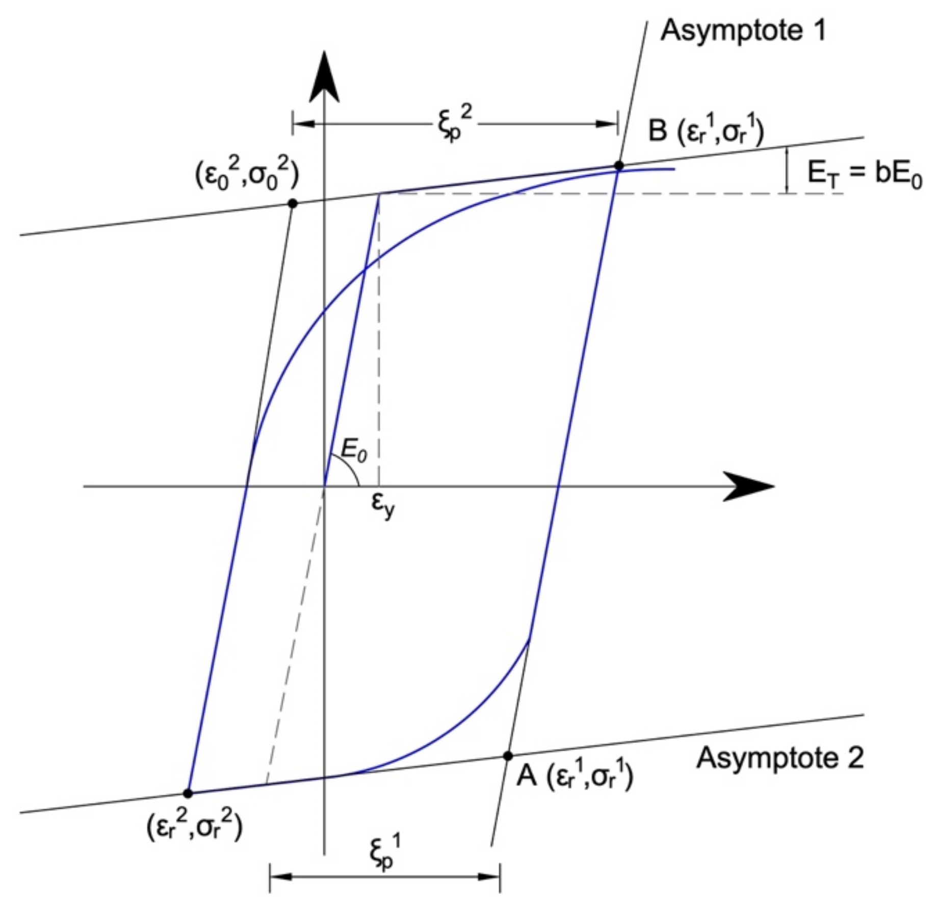
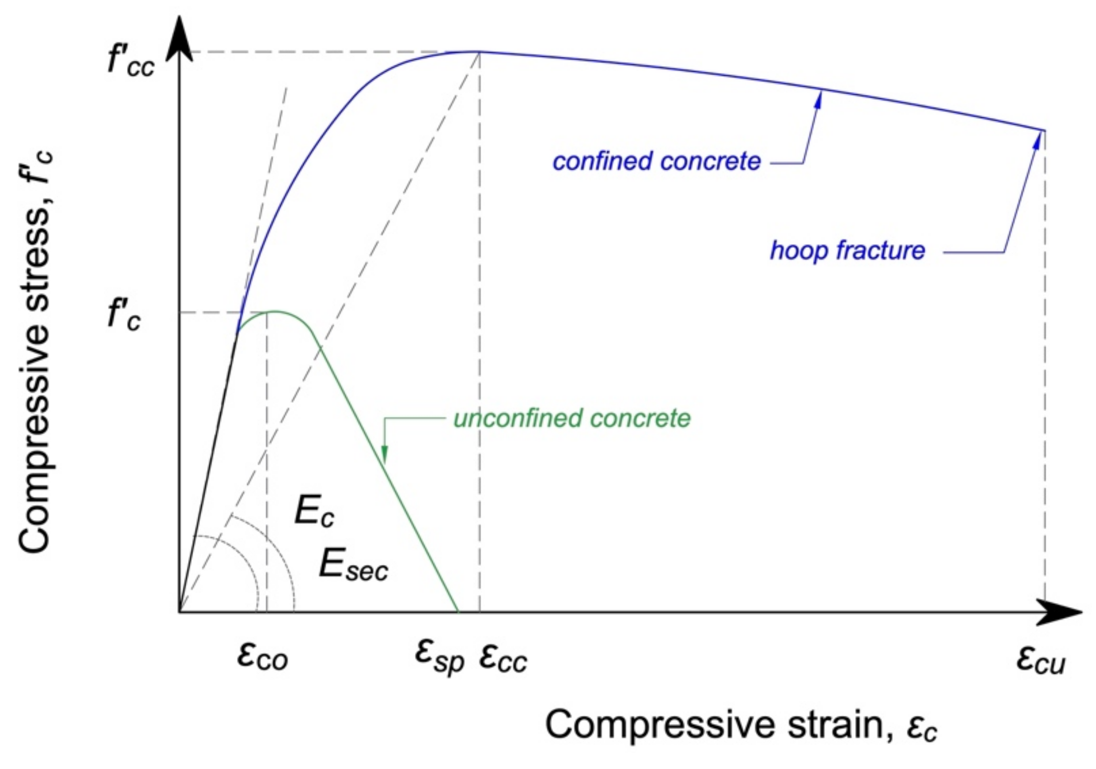
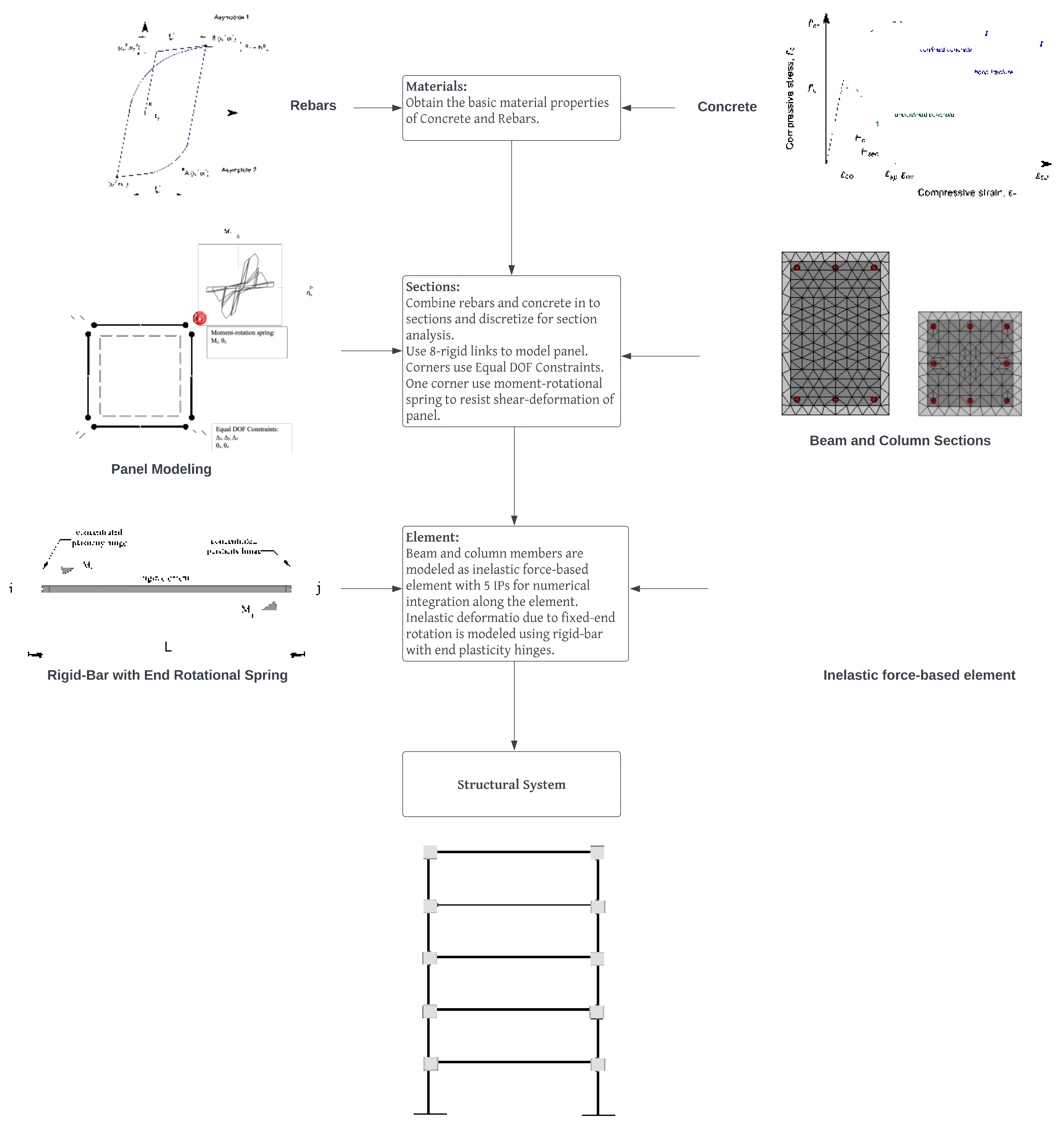
3.3.2. Material Models

The solution of Equations (32) and (33) necessitates the definition of suitable material models since a numerical solution algorithm should include stress–strain relations for concrete and reinforcing rebars for computing the section resisting forces and stiffness matrix.

The [46] nonlinear model, as updated by Filippou et al. [29] to include isotropic strain hardening, has been used in the present study to characterize the stress-strain relation of the reinforcing steel. This is the most appealing since it has the best agreement with experimental data and is computationally efficient. The stress-strain model takes on the following form to describe a curved transition from a straight-line asymptote with slope E₀ to another asymptote with slope bE₀, and allowing a good representation of the Bauschinger effect:

$${\sigma }^{*}=b{\epsilon }^{*}+\frac{\left(1-b\right){\epsilon }^{*}}{{\left[1+{\left({\epsilon }^{*}\right)}^R\right]}^{\frac{1}{R}}}$$

(41)

$${\sigma }^{*}=\frac{\left(\sigma -{\sigma }_r\right)}{\left({\sigma }_0-{\sigma }_r\right)}$$

$${\epsilon }^{*}=\frac{\left(\epsilon -{\epsilon }_r\right)}{\left({\epsilon }_0-{\epsilon }_r\right)}$$

$$R^n=R_0-\frac{a_1{\xi }_p^n}{\left(a_2+{\xi }_p^n\right)}$$

$${\xi }_p^n={\epsilon }_r^n-{\epsilon }_y^n$$

where σ^* and ε^* are the normalized stress and strain, σ_o and ε_o are the stress and strain at first yielding, b is the strain hardening, σ_r and ε_r indicate the stress and the strain at the point of the last strain reversal where the stress of equal sign took place, R is the curvature parameter, R₀ is the value of R during the first loading, a₁ and a₂ are experimentally determined parameters, and ${\xi }_p^n$ is the plastic excursion at the current semicycle (Figure 9). Fragiadakis et al. [47] provide more in-depth information on the model’s numerical implementation that also takes into consideration the buckling of steel bars.

In order to compute the concrete compressive forces, the cross-section can be divided into layers, and the distribution of concrete strain is determined assuming a linear distribution of concrete strain increments and strain increment compatibility between steel and concrete. For this purpose, a nonlinear constant confinement concrete model (Figure 10), which is a uniaxial nonlinear model that is based on the constitutive relationship proposed by Mander et al. [48] with modifications made by Martinez-Rueda and Elnashai [49] for the purpose of maintaining numerical stability under large deformations, has been used to determine the stress in each layer. The ratio of the compressive stress of confined concrete to unconfined concrete defines the constant confinement factor. Given the effective confined concrete core area A_e (mid-way through two consecutive stirrups) and area of concrete core A_cc, the effective confinement factor K_e is determined:

$$K_e=\frac{A_e}{A_{cc}}=\frac{A_e}{A_c\left(1-{\rho }_{cc}\right)}$$

(42)

$$A_e=\left(b_c{d}_c-{\displaystyle \sum }_{i=1}^n\frac{{\left(w_i^{\prime }\right)}^2}{6}\right)\left(1-\frac{s^{\prime }}{2b_c}\right)\left(1-\frac{s^{\prime }}{2d_c}\right)$$

where ρ_cc is the ratio of area of longitudinal reinforcement to the area of the core section, A_c is the area of the core of the section enclosed by the center lines of the perimeter tie, b_c and d_c are the core dimensions to the centerlines of the perimeter lateral tie, $w_i^{\prime }$ is the ith clear distance between adjacent longitudinal bars, s’ is the clear vertical spacing between lateral ties. Figure 11 illustrates a concrete model for both confined and unconfined concrete based on the stress–strain relation proposed by Mander et al. [48], which gives the longitudinal compressive concrete stress:

$$f_c=\frac{f_{cc}^{\prime }xr}{r-1+x^r}$$

(43)

$$x=\frac{{\epsilon }_c}{{\epsilon }_{cc}}$$

$${\epsilon }_{cc}={\epsilon }_{co}\left[1+5\left(\frac{f_{cc}^{\prime }}{f_{co}^{\prime }}-1\right)\right]$$

$$r=\frac{E_c}{E_c-E_{sec}}$$

$$E_{sec}=\frac{f_{cc}^{\prime }}{{\epsilon }_{cc}}$$

$$E_c=5000\sqrt{f_{co}^{\prime }} \mathrm{MPa}$$

The cover concrete has been designated as unconfined concrete, and the stress–strain behavior of the segment of the falling branch in the area where ε_c > 2ε_co is considered to be a straight line that reaches zero stress at the spalling strain ε_sp.

The confined compressive strength $f_{cc}^{\prime }$ is determined, assuming the confined concrete core is placed under triaxial compression with equal effective lateral confining forces $f_l^{\prime }$ from lateral ties:

$$f_{cc}^{\prime }=f_{co}^{\prime }\left(-1.254+2.254\sqrt{1+\frac{7.94f_l^{\prime }}{f_{co}^{\prime }}}-2\frac{f_l^{\prime }}{f_{co}^{\prime }}\right)$$

(44)

$$f_{lx}^{\prime }=K_e{\rho }_x{f}_{yh}$$

$$f_{ly}^{\prime }=K_e{\rho }_y{f}_{yh}$$

$${\rho }_x=\frac{A_{sx}}{s{d}_c}$$

$${\rho }_y=\frac{A_{sy}}{s{b}_c}$$

where f_yh is the yield strength of the transverse reinforcement, A_sx and A_sy are the total area of transverse bars running in the x and y directions respectively, $f_{lx}^{\prime }$ and $f_{ly}^{\prime }$ the effective lateral confining stresses in the x and y directions respectively. In tension, a linear stress-strain relationship is assumed up to the tensile strength, provided the tensile strength has not been exceeded. However, it can be ignored for pre-cracked member with zero tensile strength. The cyclic loading stress-strain response is assumed to be enclosed by the monotonic loading stress-strain curve (Figure 10).

When the transverse reinforcement confining the core fractures, it is regarded as the ultimate limit to confined concrete compression strain. This may be determined by comparing the increase in the strain energy absorbed by the concrete over the value suitable for unconfined concrete to the strain-energy capacity of the confining steel. The following equation for the ultimate compression strain for confined concrete may be derived by assuming that the ultimate strain of the unconfined concrete is 0.004:

$${\epsilon }_{c,dc}=0.004+1.4\frac{{\rho }_v{f}_{yh}{\epsilon }_{su}}{f_{cc}^{\prime }}$$

(45)

where ε_su is a strain value at fracture of lateral confining ties, and ρ_v is the volumetric confinement ratio, which is the sum of ρ_x and ρ_y.

3.3.3. Geometric Nonlinearity

Large displacements, large rotations, and large independent deformations relative to the chord of the frame element cause nonlinearities in kinematic quantities, and these sources of nonlinearity are referred to as geometric nonlinearities, also known as p-delta effects. These nonlinearities are negligible under normal load conditions, but they become significant in the presence of extreme loads and in large/slender structures. The internal forces demand is amplified under large lateral deflections, which results in a reduction in the effective lateral stiffness. The potential capacity of the structure to resist lateral loads decreases as internal forces rise, resulting in a drop in the structure’s effective lateral strength. Since they may eventually result in the loss of lateral resistance, ratcheting, and dynamic instability, this warrants consideration in numerical models [51].

A total co-rotational formulation developed by Correia and Virtuoso [52] is used to take into account the large displacements/rotations and large independent deformations relative to the chord of the frame elements in the model. The total co-rotational formulation makes use of an exact description of the kinematic transformations associated with large displacements and three-dimensional rotations of the element. As a result, the independent deformations and forces of the element are correctly defined, and the effects of geometric non-linearities on the stiffness matrix are naturally defined. The use of this formulation takes into account small deformations in relation to the element’s chord without losing its generality, despite the existence of large nodal rotations and displacements.

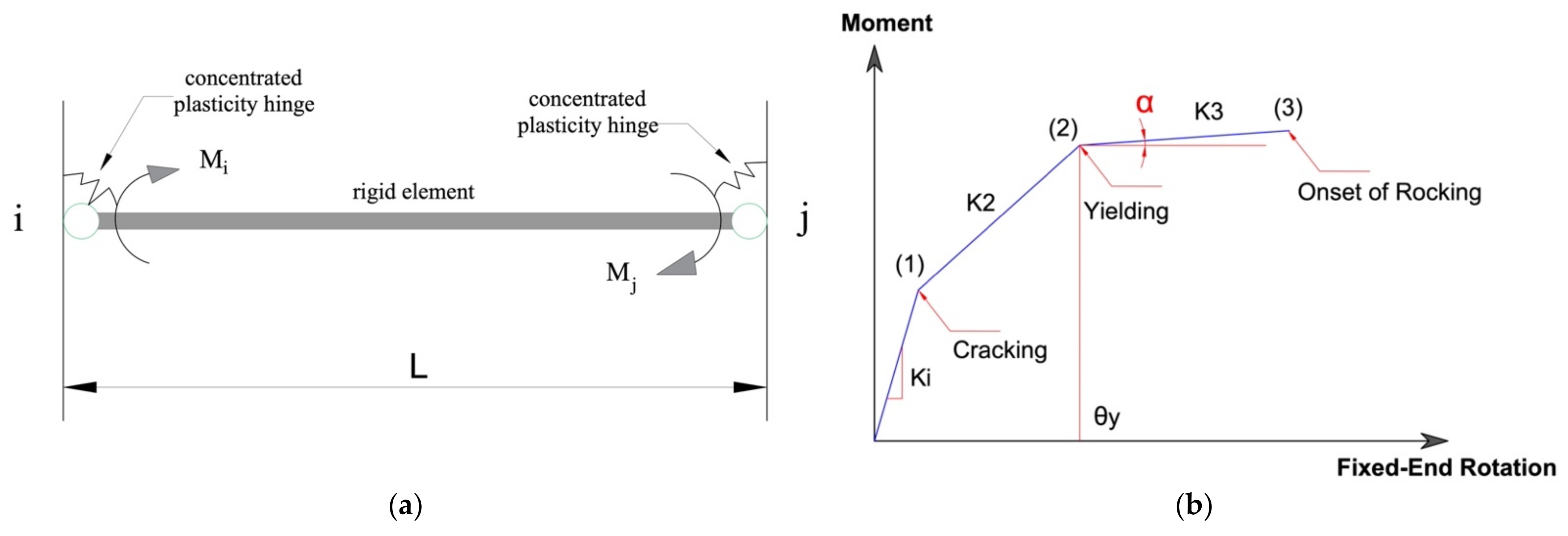
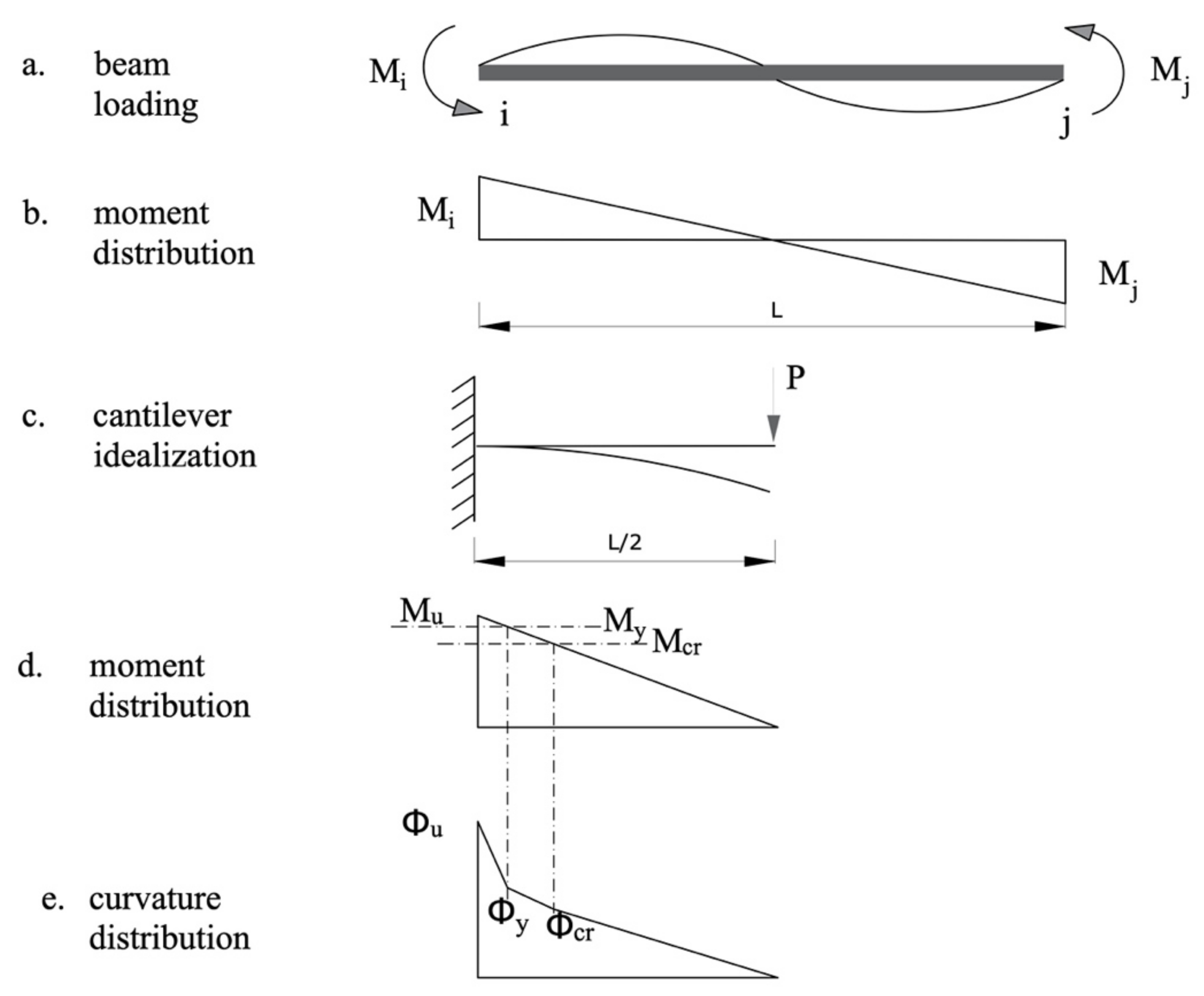
3.4. Modeling of Fixed-End Rotation

The fixed-end rotation at the interface of the beam and column caused by bond failure, longitudinal rebar-slip, and inelastic extension is simulated for each element using a single nonlinear rotational spring located at the beam–column member ends (Figure 11a), and a concentrated plasticity hinge with a nonlinear moment–rotational behavior (Figure 11b,

Table 1. Proposed moment–rotation values for fixed-end rotational spring to model beam–column member rigid-body rotational deformation [50].

Parameter	θcr (rad)	Mcr/Mmax *	θy (rad)	My/Mmax *	α = K3/K1
Value	0.00091	0.27	0.01177	0.76	0.055

* M_max is the beam maximum moment capacity.

) is used to model the rigid-body rotational deformation of the member. The formulation developed herein for fixed-end rotation is similar to the rigid-bar rotation model proposed by Filippou and Issa [30], with the improvement including a more realistic representation of the moment–rotation relationship developed recently by Ahmad et al. [50] based on quasi-static cyclic tests performed on full-scale beams exhibiting fixed-end rotation. A trilinear force–deformation envelope is proposed to model inelastic mechanisms (cracking, yielding, and rocking) with a deteriorating hysteretic rule for model stiffness and strength deterioration and pinching behavior. Due to its high initial stiffness, the hinge may only contribute marginally before the beam yields but contributes significantly after the rocking mode is initiated.

The flexibility matrix’s off-diagonal components may simply be demonstrated to be zero in this situation and as a result, the flexibility matrix of the element is given:

$$F_{FER}=\left[\begin{array}{c}{f}_i 0\\ 0 f_j\end{array}\right]$$

(46)

where f_i is the flexibility coefficient of the rotational spring at the end i and f_j is the flexibility coefficient of the rotational spring at end j. Assuming that the point of inflection remains fixed and lies in the middle of the beam throughout the loading history, in this case, each half of the member can be viewed as a cantilever beam and the flexibility coefficients can be easily formulated. The problem can be further simplified, ignoring gravity load, this corresponds to a cantilever beam subjected to load P (Figure 12).

To determine the flexibility coefficients of the concentrated hinge, the rotation at the cantilever’s root (beam ends) caused by the curvature distribution is first determined for various values of the load P, and if the moment-curvature relation is known, this can be simplified. The moment-rotation relationship proposed (Figure 11b) is trilinear, due to which the approach produces a nonlinear flexibility coefficient of the corresponding concentrated spring. The stiffness of the hinge can be determined as:

$$K_i=\frac{M_{cr}}{{\theta }_{cr}} 0\le M\le M_{cr}$$

(47)

$$K_2=\frac{M_y-M_{cr}}{{\theta }_y-{\theta }_{cr}} M_{cr}\le M\le M_y$$

(48)

$$K_3=\frac{M-M_y}{\theta -{\theta }_y} M_y\le M$$

(49)

where K_i is the initial stiffness, K₂ is the post-cracking stiffness, and K₃ is the post-yield stiffness of the hinge. The limit state values of moment (M) and rotation (θ) are given in Table 1.

It is typical to represent the flexibility matrix of a rotational spring stiffness K in terms of the prismatic beam element’s elastic stiffness for convenience:

$$K_i=\frac{4.EI}{\gamma .L}$$

(50)

$$K_2={\beta }_1\frac{4.EI}{\gamma .L}$$

(51)

$$K_3={\beta }_2\frac{4.EI}{\gamma .L}$$

(52)

where γ, β₁, and β₂ are coefficient vary as a function of the moment-rotation demand. The experimental data suggests β₁ = 0.165 and β₂ = 0.055, and γ = 0.406 if EI is based on the nominal moment and yield curvature of the beam section [50]. The flexibility matrix can be formulated as given:

$$F_{FER,1}=\frac{L}{6EI}\left[\begin{array}{c}1.5{\gamma }_i 0\\ 0 1.5{\gamma }_j\end{array}\right] 0\le M\le M_{cr}$$

(53)

$$F_{FER,2}=\frac{L}{6EI.{\beta }_1}\left[\begin{array}{c}1.5{\gamma }_i 0\\ 0 1.5{\gamma }_j \end{array}\right] M_{cr}\le M\le M_y$$

(54)

$$F_{FER,3}=\frac{L}{6EI.{\beta }_2}\left[\begin{array}{c}1.5{\gamma }_i 0\\ 0 1.5{\gamma }_j\end{array}\right] M_y\le M$$

(55)

This concentrated plasticity model has the advantage of being computationally simple can be readily implemented in a finite element computer program and can accurately represent the hysteretic response of RC members whose behavior is controlled by fixed-end rotation. The flexibility matrix of the element is calculated by simply adding the flexibility matrices of the constituent elements (i.e., beam-column inelastic member and concentrated plasticity hinge), since the plasticity hinge element and the inelastic beam-column member act in series.

3.5. RC Beam–Column Frame Member Shear Strength

3.5.1. Basics of RC Member Shear Strength

A key element of nonlinear modeling is including the most probable inelastic deformation mechanisms; therefore, the model should specify aspects for evaluating the performance of RC frames, especially when the shear failures of columns can anticipate the failure of the buildings. A comparison of the beam/column members’ flexural and shear strengths is required to ascertain if flexural or shear failure is predicted. If individual member shear deformation is negligible, less detailed modeling is appropriate, provided that members do not develop shear forces that overwhelm the capacity of the member, as this will result in a brittle mechanism and the rapid deterioration of the member’s stiffness and strength. Although shear damage was not noticed in the beam and column members for the present test specimen, since the members had sufficient shear strength and the mechanism of joint shear occurred owing to joint-region weakness, the member shear modeling is included for completeness.

It is advised that member shear strength be determined using more suitable equations that illustrate the dependence of shear strength on flexural ductility. The seismic shear strength model of columns proposed by Priestley [27] is discussed, which presents shear strength as the product of the concrete strength contribution (V_C), a truss mechanism of the transverse steel (V_S) assuming a 30° angle between the diagonal compression struts and the longitudinal axis of the column, and an arch mechanism for the axial load (V_P):

$$V_n=V_C+V_S+V_P$$

(56)

$$V_C=0.8A_{g}k\sqrt{f_c^{\prime }}$$

(57)

$$V_S=\frac{A_v{f}_{yh}\left(D-c\right)}{s}\cot {30}^{°}$$

(58)

$$V_P=P\tan \alpha$$

(59)

$$\tan \alpha =\frac{D-c}{2a}$$

where A_g is the gross area of section, k is the degradation factor dependent on the curvature ductility, f_c′ is the compressive strength of concrete, D is the depth of the section, c is the neutral axis depth, A_v is the total area of transverse reinforcement, s is the spacing of the lateral ties, f_yh is the yield strength of the transverse reinforcement, and a is shear span or distance from the maximum moment to the point of inflection. The value of k varies approximately from 3.50 [psi units] to 1.20 [psi units] as the member displacement ductility varies from one to three for bi-axial loading and two to four for uni-axial loading, respectively. As a result, the concrete contribution drops to as little as one-third of its initial value as the displacement ductility increases. The magnitude of the member flexural and shear strengths influence whether shear or flexural failure occurs and consequently, the ultimate section curvature ductility. The initial and residual shear strengths are represented by the two limiting values, V_ni and V_nd, respectively. Brittle shear failure happens when the shear force V_f, related to the initial flexural strength, is greater than V_ni. If V_f < V_nd, which ensures a ductile flexural response, the detailing of the flexural confinement determines the maximum section ductility. A shear failure is anticipated at a certain curvature ductility when V_nd < V_f < V_ni. Although the shear strength given by Equation (56) has been rather extensively used for column sections, with no axial load, it would appear that there should not be much conceptual difference between a beam and a column, and therefore Equation (56) should also immediately apply to beams. For simplicity, using Equation (57), with k = 2.40 [psi units] for curvature ductility < 3 and k = 0.60 [psi units] for curvature ductility > 7, determine the shear strength of a negative moment plastic hinge in beams.

3.5.2. Shear Strength Model Implementation

For implementation in nonlinear modeling, the shear capacity of an RC column is determined according to ASCE 41-17 [53], whereas the shear capacity of the beam section is determined according to ACI 318-19. For columns, the shear strength V_Col [psi units] shall be permitted to be calculated as:

$$V_{Col}=k_{nl}{V}_{Col0}$$

(60)

$$V_{Col0}={\alpha }_{Col}\left(\frac{A_v{f}_{ytL/E}d}{s}\right)+\lambda \left(\frac{6\sqrt{f_{cL/E}^{\prime }}}{M_{UD}/V_{UD}d}\sqrt{1+\frac{N_{UG}}{6A_g\sqrt{f_{cL/E}^{\prime }}}}\right)0.8A_g$$

(61)

where k_nl = 1.0 for displacement ductility demand is less than or equal to 2, 0.7 for displacement ductility greater than or equal to 6 and varies linearly for displacement ductility between 2 and 6, λ = 1.0 for normal-weight aggregate concrete, N_UG is the axial compression force, M_UD/V_UDd is the largest ratio of moment to shear times effective depth for the column under design loadings but shall not be taken as greater than 4 or less than 2, α_Col = 1.0 for s/d ≤ 0.75, 0.0 for s/d ≥ 1.0, and varies linearly for s/d between 0.75 and 1.0.

Equation (22.5.1.1) of ACI 318-19 is used to calculate the shear capacity of beam sections: Equation (22.5.8.5.3) of ACI 318-19 computes the shear strength provided by transverse reinforcement, and Section 22.5.5.1 of ACI 318-19 provides equations for the shear strength provided by concrete:

$$V_C=\left[2\lambda \sqrt{f_c^{\prime }}+\frac{N_u}{6A_g}\right]b_{w}d A_v\le A_{v,min}$$

(62)

$$V_C=\left[8\lambda {\left({\rho }_w\right)}^{\frac{1}{3}}\sqrt{f_c^{\prime }}+\frac{N_u}{6A_g}\right]b_{w}d A_v\le A_{v,min}$$

(63)

$$V_C=\left[8{\lambda }_S\lambda {\left({\rho }_w\right)}^{\frac{1}{3}}\sqrt{f_c^{\prime }}+\frac{N_u}{6A_g}\right]b_{w}d A_v<A_{v,min}$$

(64)

The shear strength equations (Equations (60)–(64)) were implemented in the SeismoStruct program and used to determine if the member has reached its shear capacity at each time step of the analysis. When the limit was reached, the member was assigned a residual strength (10% to 20% of maximum resistance) or remained inactive with no residual strength.

4. Validation of the Proposed Modeling Technique

4.1. Quasi-Static Cyclic Testing of Tee Beam–Column Joint

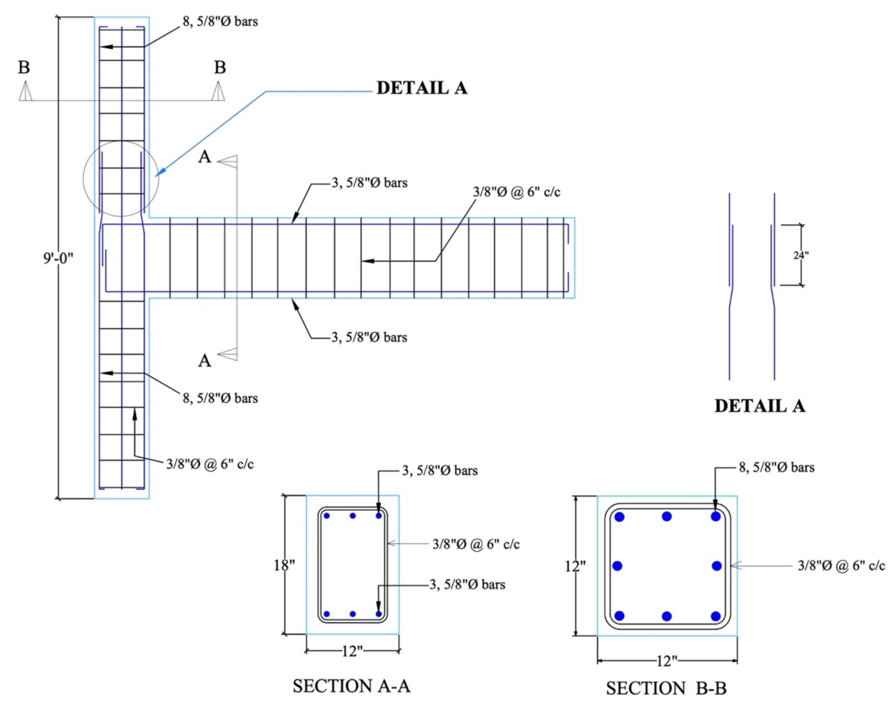
4.1.1. Description of Test Specimen

A low-rise building was considered as a prototype for choosing the geometric and reinforcement detailing of a typical substandard beam–column joint [13] in order to study the behavior of deteriorating joints and serve as a benchmark for testing and validating the proposed numerical modeling technique. Several deficiencies were discovered during the field survey of reinforced concrete building stock in Pakistan [13]. Because it was not possible to include all of the defects in the experimental models due to time and financial constraints, it was decided to analyze just those deficiencies that would have a significant influence on the seismic performance of the reinforced concrete buildings in Pakistan.

The selected beam–column joint subassembly (Figure 13) included columns that were 12 inches wide and 12 inches deep and a beam that was 12 inches wide and 18 inches deep. This model took into account all deficiencies found between design standards and actual reinforced concrete building constructions in Pakistan. These deficiencies included: spacing of ties—double of specified spacing, lack of seismic hooks, location of splice-near beam–column joint, lap length-reduced by 45%, 20% reduction in the diameter of rebars, lack of ties in the beam–column joint core (except a single tie), concrete having compressive strength of 2000 psi, and rebars having yield strength of 40,000 psi. The model’s beam was reinforced with 3#5 bars at the top and bottom to represent the use of undersized reinforcing bars in constructions. A #3 stirrup was used as the lateral tie in the beam, positioned uniformly at 6 inch on centers. There were no seismic hooks, and the ties were closed at a 90-degree angle.

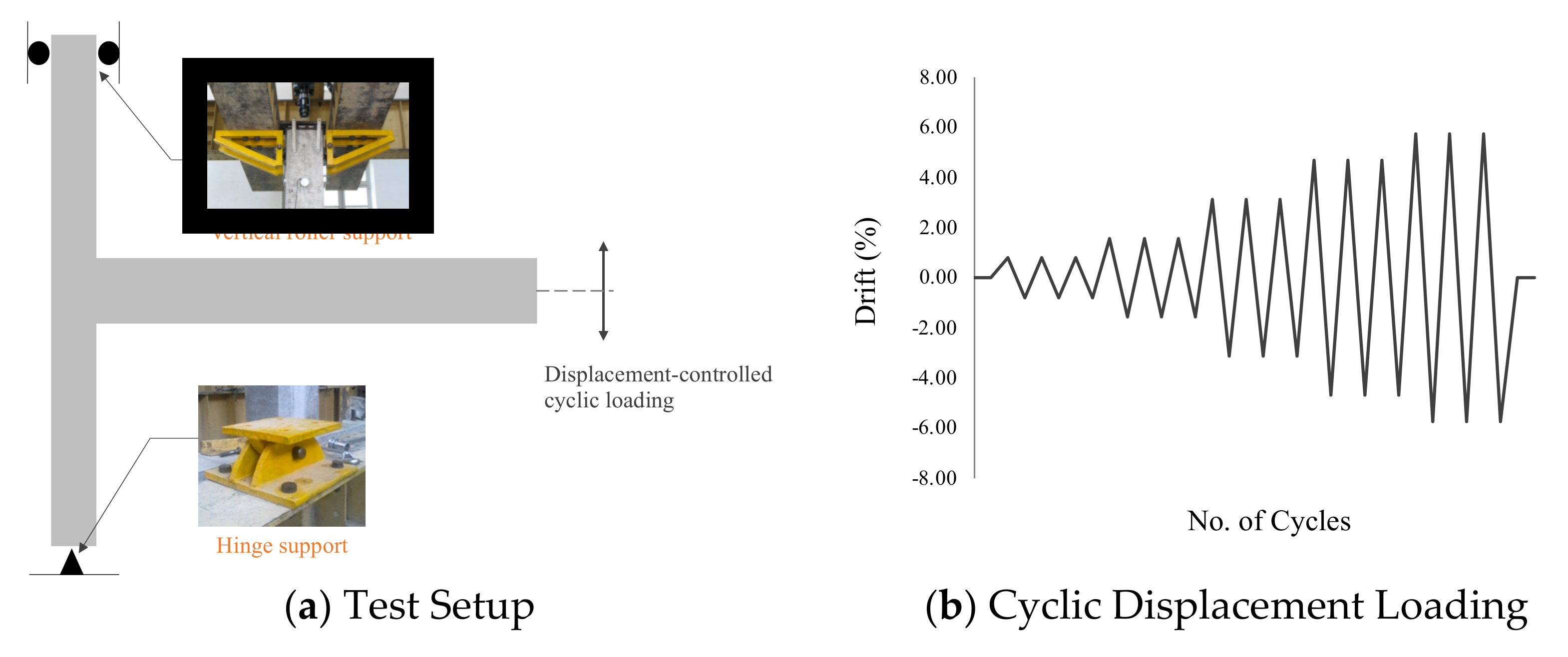
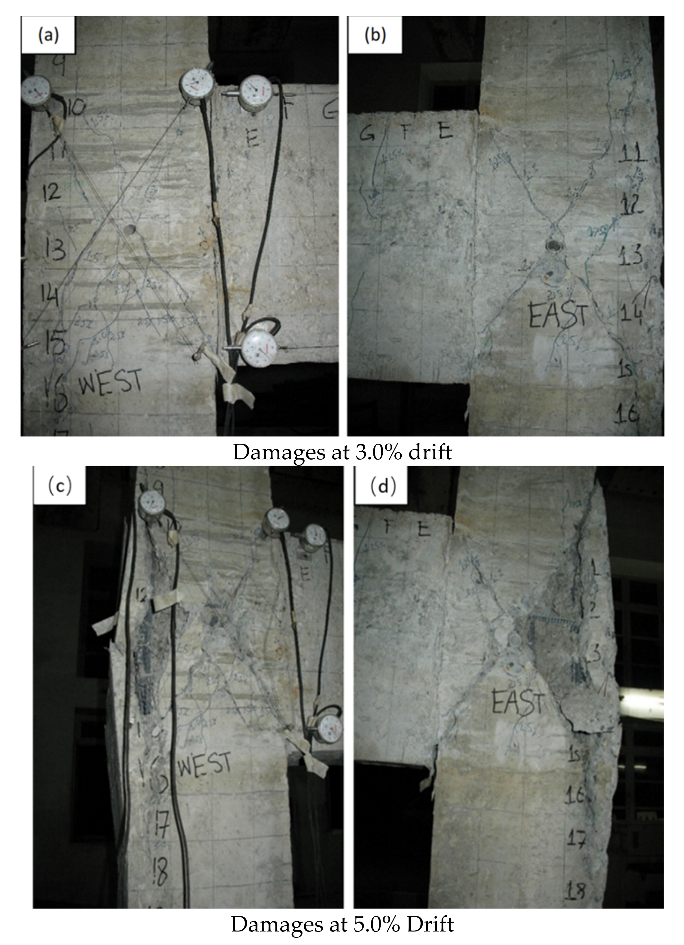
4.1.2. Experimental Program and Specimen Behavior

Figure 14 illustrates the selected test setup and loading of the beam–column joint. The load was applied directly at the point of the contra flexure of the beam (i.e., free end of T-joint). Boundary conditions were selected to accurately reflect the end restraints of a two-dimensional frame. A hinge support was used to pin-connect the bottom of the column: pins were firmly fastened to a steel girder, and that steel girder was in turn fastened to the strong floor. The top of the column was provisioned with a roller support to enable unrestricted movement in a vertical direction, while lateral movement was restricted.

A permanent gravity load of 26 tons (20% of the gross-section capacity) was applied at the top of the column. A reverse cyclic load was applied at the beam end of the beam–column assembly. To simulate the pre-cracked conditions, initially the assembly was tested under force-controlled loading. First, three tons of load was determined to be the theoretical yield capacity (F_y) of the system. This was used to guide load control testing; the force was applied in four equal increments: 0.25 F_y, 0.5 F_y, 0.75 F_y and F_y, and each increment was repeated three times. This was followed by displacement-controlled testing till the specimen attained extensive damages (Figure 15). Initially, the assembly was tested under force-controlled loading to simulate the pre-cracked conditions of existing buildings. The system’s theoretical yield capacity, F_y, was first determined to be 2.76 tons. The force was applied in four equal increments—0.25 F_y, 0.5 F_y, 0.75 F_y, and F_y—and each increment was repeated three times during the load control tests. Displacement controlled testing was conducted afterwards until the specimen had sustained extensive damages (Figure 15).

Diagonal cracks initiated in the beam–column joint and vertical cracks appeared at the beam–column interface at a drift demand of 1.0%. The existing cracks in joints became aggravated, and additional multiple cracks appeared with increasing drift demand from 1.5% to 3.0% drift. Consequently, a concrete wedge mechanism was initiated. Upon further increasing drift demand, the width of existing cracks widened, while a concrete wedge was detached from the joint at a drift demand of 5.0%. This failure mechanism is especially brittle, and the bearing load capacity was lost as a result of the pushing out of a concrete wedge; therefore, the test was terminated.

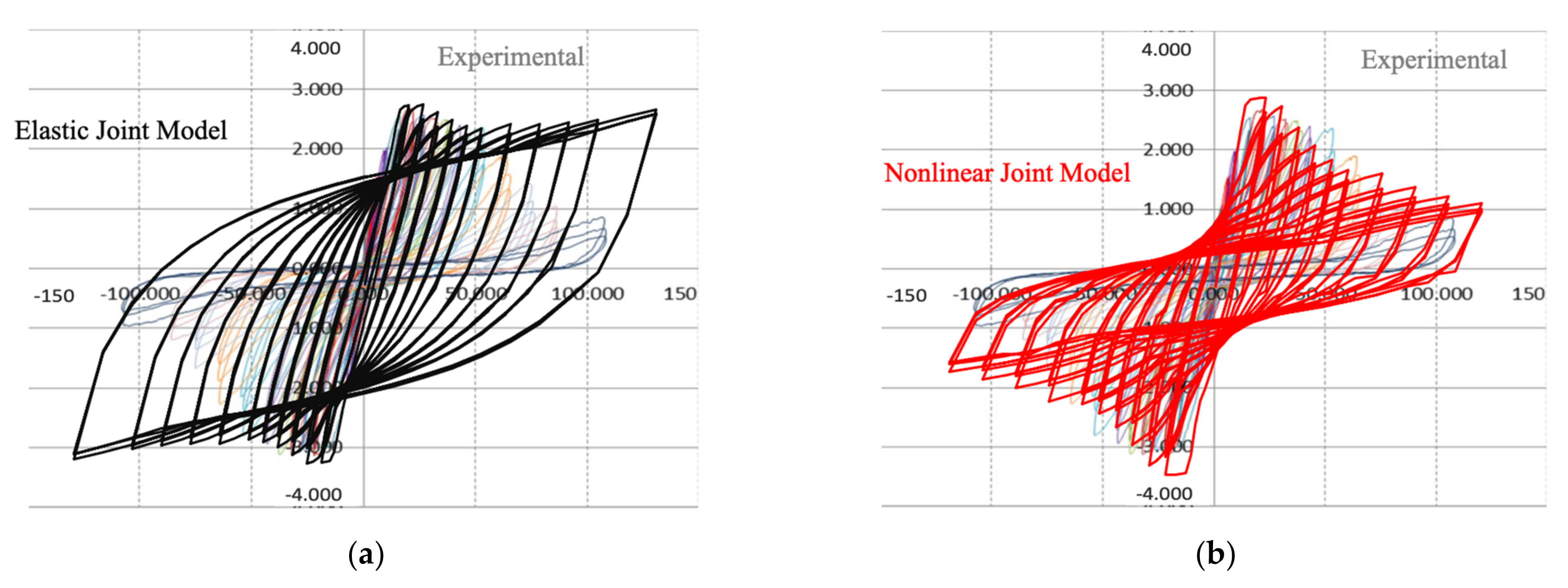
4.2. Comparison of the Numerical and Experimental Prediction

The analytical model illustrated in Figure 5 was generated using the nonlinear finite element SeismoStruct program. The analytical model is composed of the inelastic beam and column members modeled as inelastic fiber-section-based elements that use the force-based formulation with the improved materials models discussed earlier. The material model for rebars is a uniaxial steel model that was first developed by Monti et al. [54] and can comprehend the post-elastic buckling behavior of reinforcing bars in compression. It makes use of the stress–strain relationship presented by Menegotto and Pinto [46], as well as the isotropic hardening rules of Filippou et al. [29] and the buckling rules of Monti and Nuti [55]. For increased numerical stability/accuracy under transient seismic stress, it considers a further memory rule suggested by Fragiadakis et al. [47]. The material model for concrete is a uniaxial nonlinear constant confinement model described earlier that was first developed by Madas [56] and that adheres to the stress–strain relationship established by Mander et al. [48] and the cyclic rules proposed by Martinez-Rueda and Elnashai [49]. The Mander et al. [48] rule, which assumes continuous confining pressure over the whole stress–strain range, integrates the confinement effects offered by the lateral transverse reinforcement.

To simulate fixed-end rotation, a concentrated plasticity hinge was introduced at the beam end using a zero-length link element. The link element connected two contemporaneous structural nodes and necessitated the development of a separate force–displacement (or moment–rotation) response curve for each of its local six degrees of freedom. An infinitely stiff elastic force–displacement rule was assigned to all degrees of freedom, except the in-plane rotational dof that was assigned with the multilinear moment–rotation rule (Figure 11b) featuring pinching in the hysteretic force–displacement behavior to simulate the opening/closing of a vertical crack at the beam end. The selected hysteresis loop is described in Sivaselvan and Reinhorn [57], which is capable of simulating the deterioration of strength, stiffness, and bond slip. The vertical dof of the beam element and the horizontal dof of the column element were assigned with linear force–displacement behavior to idealize the member shear deformation. However, the shear strength limit criteria described earlier were used to identify member shear failure.

Four stiff link elements were positioned along the edges of the panel to idealize the joint panel, and one nonlinear moment–rotation spring was introduced at one corner hinge. The backbone moment–rotation curve represents the behavior for monotonic loading, establishes strength and deformation bounds (Figure 6a), and uses a pinched hysteretic model from Ibarra et al. [37] to model the deteriorating hysteresis of the backbone curve (Figure 6b).

Figure 16 compares the analytical and experimental hysteretic responses of the Tee beam–column joint. This demonstrates that the initial stiffness, maximum strength, and hysteretic response of the analytical model agree well with the experimental response. The proposed joint modeling technique accurately simulates the inelastic response of the Tee beam–column joint viz. the plastic hinge flexural damage mechanism, with the slip of the reinforcing bars in the inelastic beam member and joint damage shear hinge mechanism within the panel zone, as well as the deterioration of stiffness and strength important for the considered substandard beam–column joint. Therefore, the proposed joint panel idealization using a nonlinear zero-length rotational spring with a deteriorating hysteretic rule may accurately model the nonlinear behavior of the exterior beam–column joints in existing structures.

5. Frame Structure Nonlinear Response Analysis

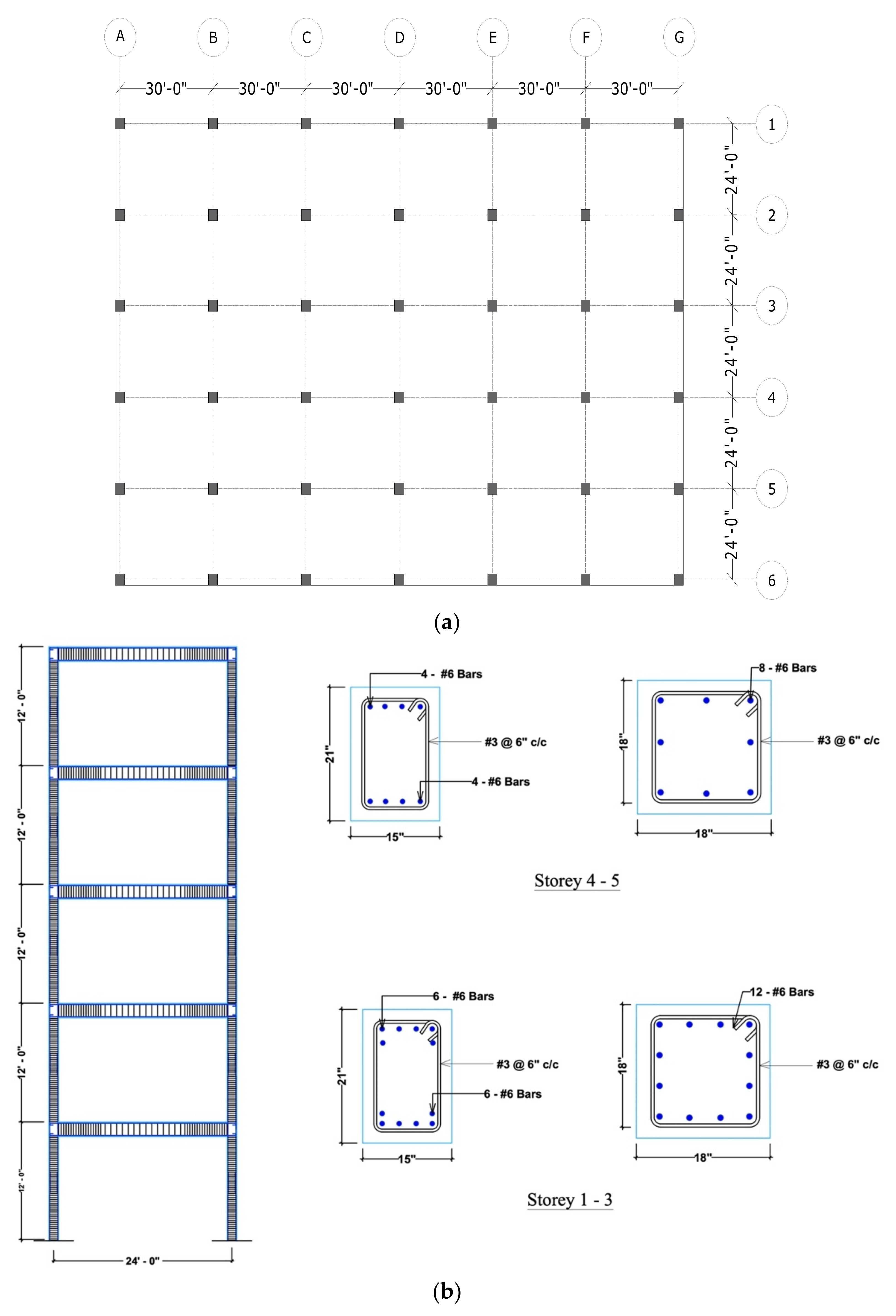
5.1. Description of Frame Structure

A five-story reinforced concrete moment-resisting frame structure in the present study serves as a representative example of a Pakistani substandard frame building construction that falls short of code requirements (Figure 17). The assumed footprint of the structure is 45.72 m (150 ft) by 36.576 m. (120 ft). The structure has five bays in each direction, with the following dimensions: 9.144 m (30 ft) longitudinal bay width, 7.3152 m (24 ft) transverse bay width, and 3.6576 m story height (12 ft).

In compliance with the building regulations, a live load of 2.40 kN/m² was used. A 203 mm (8 in)-thick two-way floor slab and a superimposed dead load of 1.0 kN/m² (20 lbs/ft²) were included in the dead load, in addition to the members’ self-weight. The beams and columns were designed using regular reinforced concrete with a 28-day unconfined compressive strength of 13.80 MPa (2000 psi). The weight of the concrete was taken 23.60 kN/m³ (150 lbs/ft³). Reinforcement steel of grade 40 with a design yield tensile strength of 276 MPa (40 ksi) was used. Building analysis and design were performed for the short direction in accordance with BCP-SP (2007), assuming a fixed base to signify an adequate foundation.

A single-bay, two-dimensional, multi-story frame was extracted for nonlinear modeling and building response analysis. Based on the tributary area, weights were applied to the single-bay frame. Due to the same structural and dynamic properties that follow (i.e., building vibration period, frame damage mechanisms, and nonlinearities), it was intended that the behavior of the buildings resemble that of a planar frame. While other 3-dimensional effects and the slab/joists contribution can affect a structure’s seismic response [58,59,60], the planar frame simplification allows for a significant reduction in the number of elements and degrees of freedom in the numerical model, which reduces the computation time needed for the building nonlinear response analysis and is a conservative approach to assessment.

5.2. Numerical Modeling

The nonlinear finite element SeismoStruct program was used to numerically model the considered prototype multi-story frame in a manner similar to the Tee beam–column joint discussed earlier. The floor loads and masses were lumped evenly at floor structural nodes. In order to account for the large displacements, the total corotational geometric transformation was used [52]. According to earlier research, the mass and stiffness proportional Rayleigh damping in the first two modes was set at 2% of critical for the considered frame Ahmad et al. [61]. The building frame elements were discretized using the fiber-section-based element with mixed formulation developed by Spacone et al. [40,42] that uses the improved material model formulations [47,49]. To account for the fixed-end rotation caused by bond failure, rebars yielding, and inelastic extension, the frame elements were provided with concentrated plasticity hinges that maintain the formulation of Filippou et al. [29] and uses the pinched degrading hysteretic rule as proposed by Sivaselvan and Reinhorn [57]. The frame was idealized using elastic joints (center-line model) and nonlinear joint panel models with the deterioration of stiffness and strength to evaluate the significance of the improved formulation. The joint panels were idealized as a parallelogram of stiff elements and provisioned with a corner nonlinear moment–rotation spring that uses the pinched deteriorating hysteresis of Ibarra et al. [37].

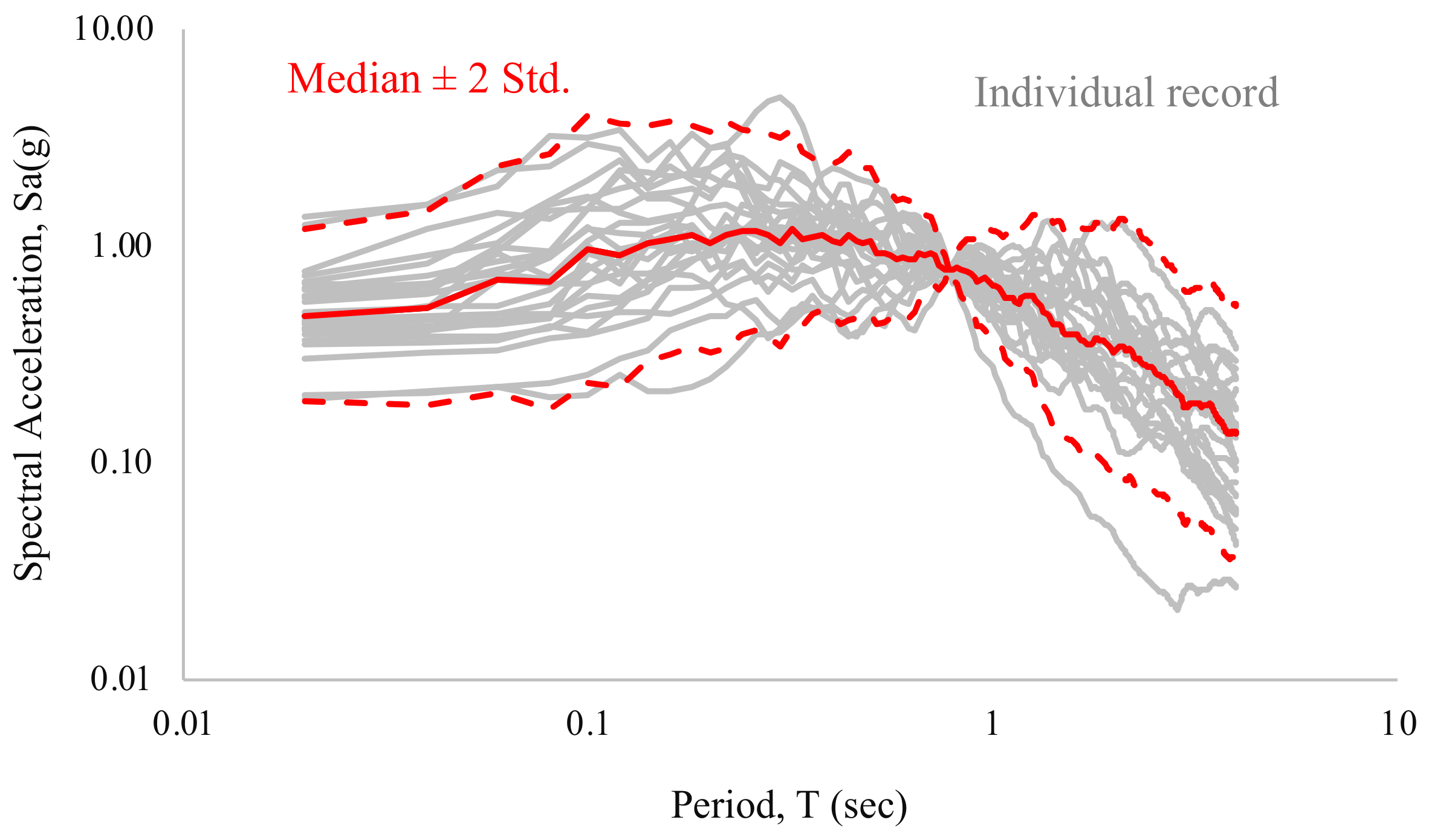
5.3. Selected Ground Motions

Twenty-four far-fault earthquake ground motions were obtained from the PEER NGA online ground motion database. Given that an existing structure may experience a variety of moderate-to-strong ground motions throughout its design life, it was preferable to subject the numerical model to a range of ground motions that represented variation in the key seismological parameters, such as magnitude (Mw: 6 to 7.62), fault mechanism (reverse, reverse-oblique, and strike-slip), source-to-site distance (Rjb: 17 km to 29 km), and significant duration (D5-95%: 11 s to 70. A single ground motion from each earthquake event was chosen in order to account for record-to-record variability. Earthquake events from numerous active tectonic zones (US, Japan, New Zealand, Iran, Taiwan, Armenia, Mexico) were taken into consideration. The median spectrum for the elastic 5% damped single degrees of freedom systems with periods ranging from 0.02 s to 4.0 s and subjected to unscaled ground movements is shown in Figure 18 and reported

Table A1. Details of the ground motions used for nonlinear response history analysis. Rev. represents reverse faults; Rev. Ob. represents reverse and oblique faults, and SS represents strike-slip faults.

S. No.	Earthquake Event	Year	Recording Station	Mw	Fault	Rjb (km)	Duration (s), 5–95%
1	San Fernando	1971	LA–Hollywood Stor FF	6.61	Rev.	22.77	13.4
2	Tabas_ Iran	1978	Boshrooyeh	7.35	Rev.	24.07	19.5
3	Coalinga-01	1983	Parkfield–Fault Zone 15	6.36	Rev.	28.00	19.7
4	Spitak_ Armenia	1988	Gukasian	6.77	Rev. Ob.	23.99	10.5
5	Loma Prieta	1989	Hollister–South & Pine	6.93	Rev. Ob	27.67	28.8
6	Northridge-01	1994	LA–W 15th St	6.69	Rev.	25.59	20.2
7	Chi-Chi_ Taiwan	1999	CHY025	7.62	Rev. Ob.	19.07	35.3
8	St Elias_ Alaska	1979	Icy Bay	7.54	Rev.	26.46	34.6
9	Niigata_ Japan	2004	NIG018	6.63	Rev.	21.55	70.3
10	Chuetsu-oki_ Japan	2007	Joetsu Kita	6.80	Rev.	28.97	30.8
11	Iwate_ Japan	2008	IWT012	6.90	Rev.	20.47	30.8
12	Christchurch_ New Zealand	2011	LINC	6.20	Rev. Ob.	18.47	13.3
13	Northern Calif-03	1954	Ferndale City Hall	6.50	SS	26.72	19.4
14	Imperial Valley-06	1979	Delta	6.53	SS	22.03	51.4
15	Victoria_ Mexico	1980	Chihuahua	6.33	SS	18.53	19
16	Morgan Hill	1984	Agnews State Hospital	6.19	SS	24.48	40.9
17	Superstition Hills-02	1987	Brawley Airport	6.54	SS	17.03	14.3
18	Landers	1992	North Palm Springs	7.28	SS	26.84	37.9
19	Kobe_ Japan	1995	Fukushima	6.90	SS	17.85	35.7
20	Tottori_ Japan	2000	OKY005	6.61	SS	28.81	24
21	Parkfield-02_ CA	2004	Coalinga–Fire Station 39	6.00	SS	22.45	27.7
22	El Mayor-Cucapah_ Mexico	2010	Chihuahua	7.20	SS	18.21	51.2
23	Joshua Tree_ CA	1992	Thousand Palms Post Office	6.10	SS	17.15	11.1
24	Darfield_ New Zealand	2010	WSFC	7.00	SS	24.36	26.2

in Appendix B. The selected unscaled ground motions have a peak acceleration of 0.35 g at a period of 0.26 s and a median peak ground acceleration of 0.16 g.

5.4. Frame Nonlinear Response

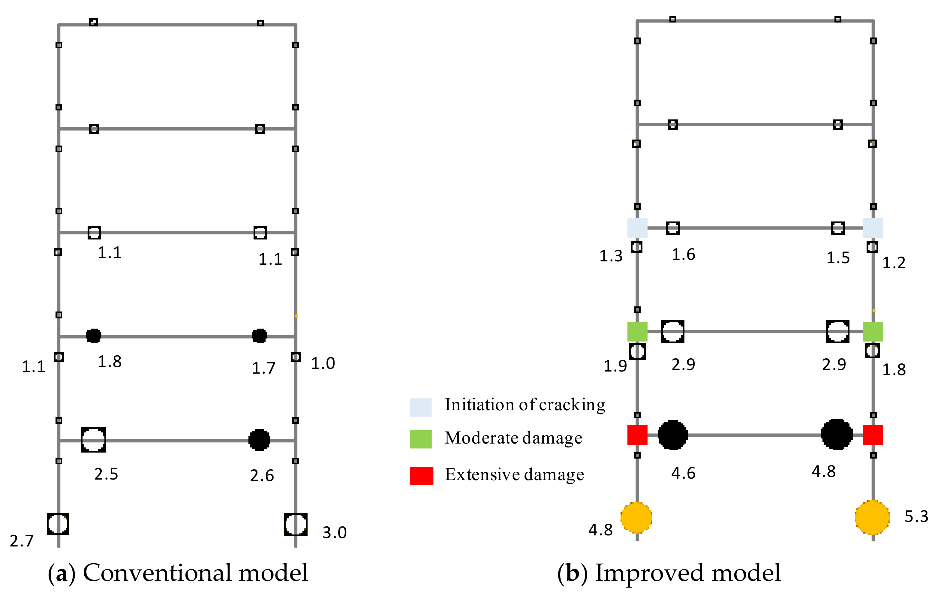
5.4.1. Damage Distribution

The seismic response of the selected frame was evaluated using a nonlinear response history analysis procedure, with both a conventional frame model with elastic joints and an improved frame model with nonlinear joint model and improved element formulation taken into account.

The ground motion of the Kocaeli Turkey earthquake of 17 August 1999 (recording station: YARIMC, KOERI330; Source: PEER Strong Motion Database) was considered and scaled linearly by a factor of 1.75 to induce large nonlinearity in the frame for contrasting the behavior of frames. Member chord rotation indicates the extent of plasticity the member experiences during ground motion, which is an important indicator of seismic damage distribution. Damage distribution diagrams were developed (Figure 19), depicting elements’ maximum chord rotation values (in percentage) to graphically compare the effects of joint modeling on the damage distribution. Shear hinge formation in the joints was also reported. The joint damage corresponded to the initiation of diagonal cracking when the principal tensile stress in the joint exceeded 0.29 (f_c′)^0.5 MPa, moderate damage when the principal tensile stress in the joint was between 0.29 (f_c′)^0.5 MPa and 0.42 (f_c′)^0.5 MPa, and extensive damages in the panel zone when the principal tensile stress in the joint exceeded 0.42 (f_c′)^0.5 MPa. Due to the flexibility that joint deformation provides, the activation of the joint shear mechanism increased the chord rotation demand on the connecting beam members. The performance of the conventional frame with elastic joints was satisfactory under the considered ground motions. The improved model, on the other hand, shows critical shear mechanism and increased member chord rotation demand sufficient to cause soft-story mechanism and consequent frame collapse.

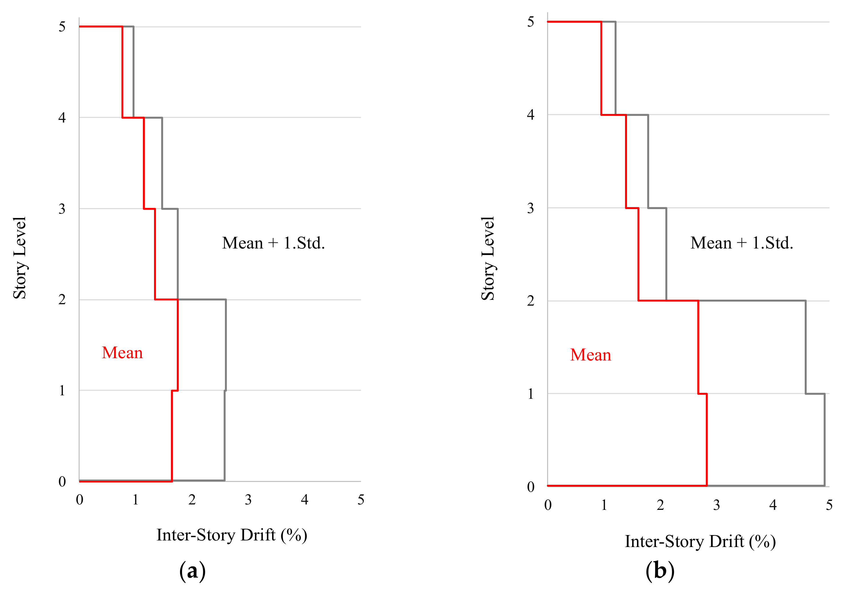
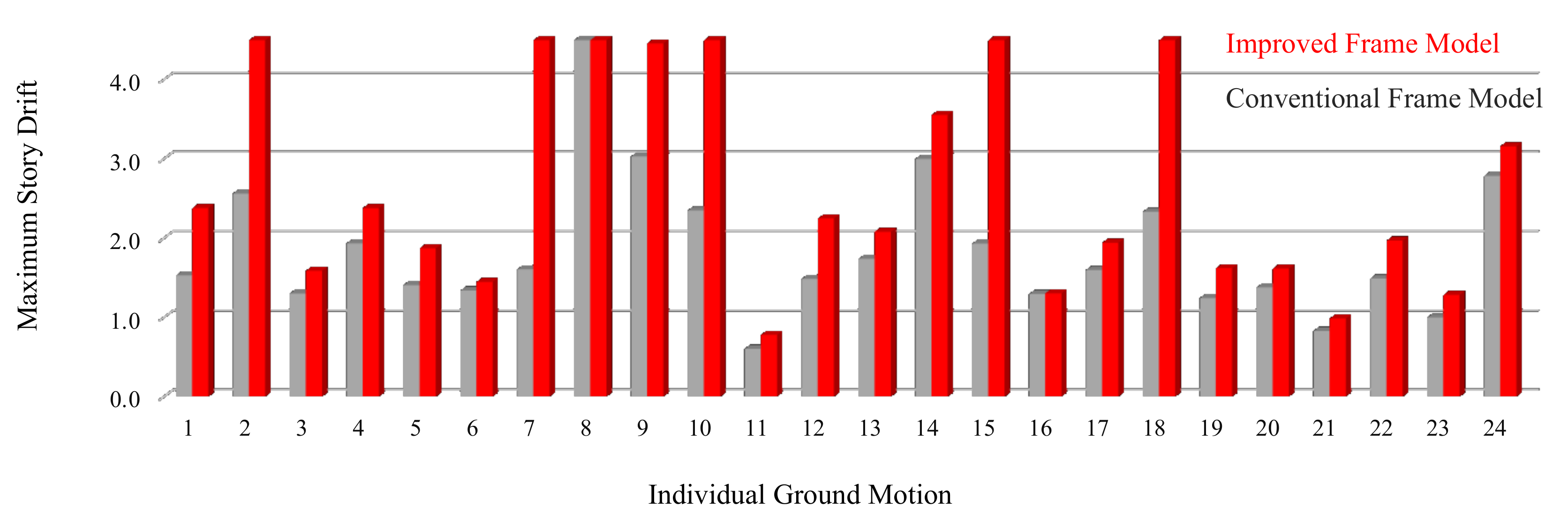
5.4.2. Inter-Story Drift Demand

The maximum inter-story drift ratio per record was obtained in order to evaluate the modeling technique with regard to the distribution of lateral deformation demand. Figure 20 shows the distribution of the maximum inter-story drift values while taking the average of the suite of ground motions. The inter-story drift distribution emphasizes the significance of the joint nonlinear model and the improved element formulation because, when compared to the drift demand for a conventional frame model, the drift demand for the frame model increases when joint nonlinearity is included and the improved element formulation is used. For the improved frame model with nonlinear joints, an increase of up to 62% (mean drift) and 89% (mean + 1.std.) is shown in the lower floors when assessing the inter-story drift distribution. As a result, the frame drift responses are drastically underestimated by the conventional frame model.

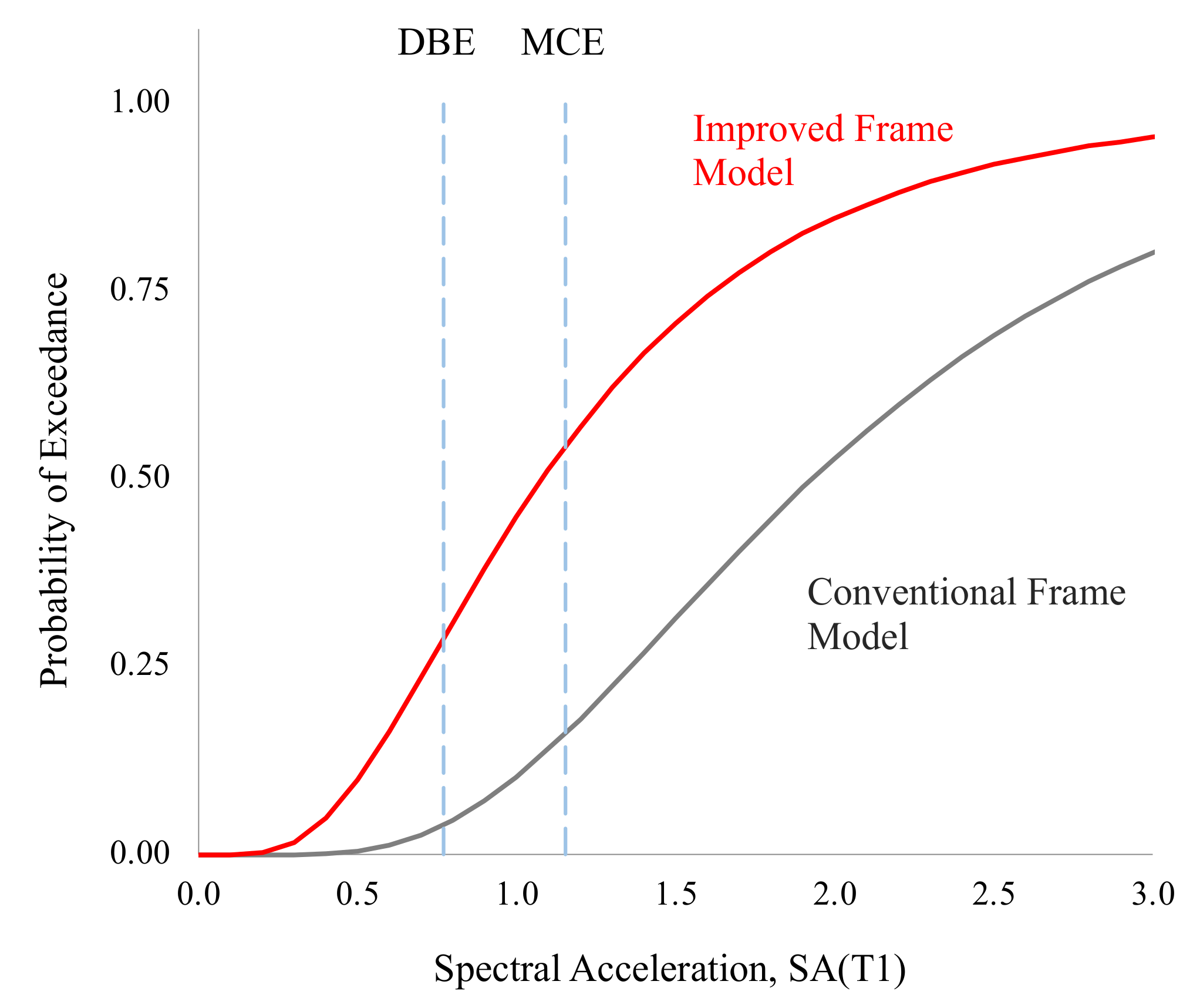
5.4.3. Collapse Risk

According to the experimental results discussed earlier, 4.50% of story drift is a realistic approximation for the beam–column connection’s collapse limit since, after this drift limit was exceeded, the joint lost its ability to support the gravity loads. Figure 21 reports the maximum story drift demand for each individual ground motion. Comparing the maximum story drift demand for different ground motions can give the instances the demand exceeds the capacity. We observed seven instances of the demand exceeding the capacity in the case of an improved frame model, resulting in a collapse risk of 7/24 = 0.292 (probability of failure = 29.20%). However, in the case of the conventional frame model, there was only one event wherein the demand exceeded the capacity, which resulted in a collapse risk of 1/24 = 0.042 (probability of failure = 4.20%). The relevant fitting procedure for fitting fragility functions that use the maximum likelihood method, as outlined by Baker [62], was used to derive fragility functions for the considered frames. Figure 22 shows the fragility functions of both conventional and improved frame models, indicating that the conventional model grossly underestimates the collapse risk of frames.

6. Conclusions

The majority of existing nonlinear modeling techniques are deficient in one or more crucial characteristics (lack of fixed-end rotation deformation or stiffness and strength deterioration due to joint shear hinge), making them less appropriate for simulating the nonlinear behavior of existing substandard beam–column joints with pre-cracks that exhibit the deterioration of stiffness and strength under cyclic loading. In order to effectively model and simulate the deteriorating response of substandard beam–column joints, as demonstrated in the experimental test and supported by numerical simulation, fixed-end rotation must be taken into consideration, in addition to joint nonlinearity. The issue with pre-cracked RC members is that they exhibit fixed-end rotation under seismic actions that considerably contribute to deformation.

To accurately determine the member stiffness matrix, resisting forces, and deformation, it is therefore necessary to improve the conventional nonlinear finite element fiber-section-based element to account for the appropriate section/element force–deformation behavior. Since only the end rotational deformation needs to be additionally included, the formulation takes into account supplementing the conventional beam–column element with an additional rigid-bar with concentrated plasticity hinges at the end.

The nonlinear response history analysis of a five-story RC frame showed that activating the joint shear hinge and fixed-end rotation mechanisms increased the chord rotation demand on the connecting beam members by up to 85%. When determining the inter-story drift demand, the collapse probability of structures subjected to design base ground motions increased from 4.20% to 29.20%.

The importance of accurate nonlinear modeling becomes evident when assessing the performance of structures for strong ground motions, as the collapse risk is grossly underestimated when using conventional modeling techniques, in contrast to a more accurate nonlinear model. It is of particular importance when determining the collapse risk of structures for strong ground shaking with a large duration, and it becomes crucial in the case of reverse/oblique faults because most collapses (five out of seven) are observed in earthquakes caused by these faults.

The formulation and modeling proposed in this research are best suited for pre-cracked beam–column members that exhibit fixed-end rotation due to rebar slip/inelastic extension and the deterioration of joint stiffness/strength. Because conventional models are applicable in most situations, they must be improved when used to assess existing structures with the issues highlighted in the present research (i.e., fixed-end rotation, joint shear hinging, and deterioration). To generalize the application of the suggested formulation to structures with joints of adequate strength and without fixed-end rotation, considering the elastic response of the joint panel and discarding the fixed-end rotational springs in modeling RC beam–column members are suggested. Although the proposed detailed modeling increases analysis time in comparison to the conventional model, it is recommended for the risk assessment of individual buildings in order to obtain detailed information that can effectively guide retrofitting efforts. As the joint deformability decreases significantly under bi-axial loading, the proposed modeling may be extended for the analysis of 3D structures.

References

1. Moehle, J.P.; Mahin, S.A. Observations on the behavior of reinforced concrete buildings during earthquakes. ACI Spec. Publ. 1991, 127, 67–90. [Google Scholar]
2. Varum, H. Seismic assessment, strengthening and repair of existing buildings. Ph.D. Thesis, Department of Civil Engineering, University of Aveiro, Aveiro, Portugal, 2003. [Google Scholar]
3. EERI. Northridge Earthquake January 17; Preliminary Reconnaissance Report, Earthquake Engineering Research Institute (EERI): Oakland, CA, USA, 1994. [Google Scholar]
4. Aycardi, L.E.; Mander, J.B.; Reinhorn, A.M. Seismic resistance of reinforced concrete frame structures designed only for gravity loads–experimental performance of subassemblages. ACI Struct. J. 1994, 91, 552–563. [Google Scholar]
5. Beres, A.; Pessiki, S.P.; White, R.N.; Gergely, P. Implications of experiments on the seismic behaviour of gravity load designed RC beam-to-column connections. Earthq. Spectra 1996, 12, 185–198. [Google Scholar] [CrossRef]
6. Gautam, D.; Adhikari, R.; Rupakhety, R. Seismic fragility of structural and non-structural elements of Nepali RC buildings. Eng. Struct. 2021, 232, 111879. [Google Scholar] [CrossRef]
7. Ahmad, N.; Shahzad, A.; Rizwan, M.; Khan, A.N.; Ali, S.M.; Ashraf, M.; Naseer, A.; Ali, Q.; Alam, B. Seismic performance assessment of non-compliant SMRF reinforced concrete frame: Shake-table test study. J. Earthq. Eng. 2019, 23, 444–462. [Google Scholar] [CrossRef]
8. Rizwan, M.; Ahmad, N.; Khan, A.N. Seismic performance of compliant and noncompliant special moment-resisting reinforced concrete frames. ACI Struct. J. 2018, 115, 1063–1073. [Google Scholar] [CrossRef]
9. Ricci, P.; De Risi, M.T.; Verderame, G.M.; Manfredi, G. Experimental tests of unreinforced exterior beam-column joints with plain bars. Eng. Struct. 2016, 118, 178–194. [Google Scholar] [CrossRef]
10. De Risi, M.T.; Verderame, G.M. Experimental assessment and numerical modelling of exterior non-conforming beam-column joints with plain bars. Eng. Struct. 2017, 150, 115–134. [Google Scholar] [CrossRef]
11. Melo, J.; Varum, H.; Rossetto, T. Experimental assessment of the monotonic and cyclic behavior of exterior RC beam-column joints built with plain bars and non-seismically designed. Eng. Struct. 2022, 270, 114887. [Google Scholar] [CrossRef]
12. ACI-352-R02. In Recommendations for the Design of Beam-Column Joints in Monolithic Reinforced Concrete Structures; American Concrete Institute (ACI): Farmington Hills, MI, USA, 2002.
13. Badrashi, Y.I. Response modification factors for reinforced concrete buildings in Pakistan. Ph.D. Thesis, Department of Civil Engineering, UET Peshawar, Peshawar, Pakistan, 2016. [Google Scholar]
14. El-Metwally, S.E.; Chen, W.F. Moment-rotation modeling of reinforced concrete beam-column connections. Struct. J. 1988, 85, 384–394. [Google Scholar]
15. Alath, S.; Kunnath, S.K. Modeling inelastic shear deformations in RC beam-column joints. In Proceedings of 10th Engineering Mechanics Conference ASCE, Boulder, Colorado, USA, 30 April 1995; pp. 822–825. [Google Scholar]
16. Biddah, A.; Ghobarah, A. Modelling of shear deformation and bond slip in reinforced concrete joints. Struct. Eng. Mech. 1999, 7, 413–432. [Google Scholar] [CrossRef]
17. Lowes, L.N.; Altoontash, A. Modeling reinforced-concrete beam-column joints subjected to cyclic loading. J. Struct. Eng. ASCE 2003, 129, 1686–1697. [Google Scholar] [CrossRef]
18. Youssef, M.; Ghobarah, A. Modelling of RC beam-column joints and structural walls. J. Earthq. Eng. 2001, 5, 93–111. [Google Scholar] [CrossRef]
19. Shin, M.; LaFave, J.M. Testing and modelling for cyclic joint shear deformations in RC beam-column connections. In Proceedings of the 10th World Conference on Earthquake Engineering, Vancouver, BC, Canada, 1 August 2004; p. 301. [Google Scholar]
20. Altoontash, A. Simulation and damage models for performance assessment of reinforced concrete beam-column joints. Ph.D. Thesis, Department of Civil and Environmental Engineering, Stanford University, Stanford, CA, USA, 2004. [Google Scholar]
21. Ning, C.L.; Yu, B.; Li, B. Beam-column joint model for nonlinear analysis of non-seismically detailed reinforced concrete frame. J. Earthq. Eng. 2016, 20, 476–502. [Google Scholar] [CrossRef]
22. Elmorsi, M.; Kianoush, M.R.; Tso, W.K. Modeling bond-slip deformations in reinforced concrete beam-column joints. Can. J. Civ. Eng. 2000, 27, 490–505. [Google Scholar] [CrossRef]
23. Pampanin, S.; Magenes, G.; Carr, A. Modeling of shear hinge mechanism in poorly detailed RC beam-column joints. In Concrete Structures in Seismic Regions: Fib, Symposium; University of Canterbury, Civil Engineering: Athens, Greece, 2003; p. 171. [Google Scholar]
24. Sharma, A.; Eligehausen, R.; Reddy, G.R. A new model to simulate joint shear behavior of poorly detailed beam-column connections in RC structures under seismic loads. Part I: Exterior joints. Eng. Struct. 2011, 33, 1034–1051. [Google Scholar] [CrossRef]
25. Kunnath, S.K.; Hoffmann, G.; Reinhorn, A.M.; Mander, J.B. Gravity-load-designed reinforced concrete buildings–Part I: Seismic evaluation of existing construction and Part II: Evaluation of detailing enhancements. ACI Struct. J. 1995, 92, 343–478. [Google Scholar]
26. Ghobarah, A.; Biddah, A. Dynamic analysis of reinforced concrete frames including joint shear deformation. Eng. Struct. 1999, 21, 971–987. [Google Scholar] [CrossRef]
27. Priestley, M.J.N. Displacement-based seismic assessment of reinforced concrete buildings. J. Earthq. Eng. 1997, 1, 157–192. [Google Scholar] [CrossRef]
28. Khan, M.S.; Basit, A.; Ahmad, N. A simplified model for inelastic seismic analysis of RC frame have shear hinge in beam-column joints. Structures 2021, 29, 771–784. [Google Scholar] [CrossRef]
29. Fillippou, F.C.; Popov, E.P.; Bertero, V.V. Effects of Bond Deterioration on Hysteretic Behaviour of Reinforced Concrete Joints; Technical Report, Report No. UCB/EERC-83/19; EERC, University of California: Berkeley, CA, USA, 1983. [Google Scholar]
30. Filippou, F.C.; Issa, A. Nonlinear Analysis of Reinforced Concrete Frames under Cyclic Load Reversals; Technical Report, Report No. UCB/EERC-88/12; EERC, University of California: Berkeley, CA, USA, 1988. [Google Scholar]
31. Baber, T.T.; Noori, M.N. Random vibration of degrading pinching systems. J. Eng. Mech. ASCE 1985, 111, 1010–1026. [Google Scholar] [CrossRef]
32. Vecchio, F.J.; Collins, M.P. The modified-compression field theory for reinforced concrete elements subjected to shear. ACI J. 1986, 83, 219–231. [Google Scholar]
33. Lowes, L.N.; Mitra, N.; Altoontash, A.A. A Beam-Column Joint Model for Simulating the Earthquake Response of Reinforced Concrete Frames; Technical Report, Report no. PEER 2003/10; Pacific Earthquake Engineering Research Center, University of California: Berkeley, CA, USA, 2004. [Google Scholar]
34. Park, R. A summary of results of simulated seismic load tests on reinforced concrete beam-column joints, beams and columns with substandard reinforcing details. J. Earthq. Eng. 2002, 6, 147–174. [Google Scholar] [CrossRef]
35. Paulay, T.; Priestley, M.J.N. Seismic Design of Reinforced Concrete and Masonry Buildings; John Wiley & Sons Inc.: New York, NY, USA, 1992. [Google Scholar]
36. Calvi, G.M.; Magenes, G.; Pampanin, S. Relevance of beam-column joint damage and collapse in RC frame assessment. J. Earthq. Eng. 2002, 6, 75–100. [Google Scholar] [CrossRef]
37. Ibarra, L.F.; Medina, R.A.; Krawinkler, H. Hysteretic models that incorporate strength and stiffness deterioration. Earthq. Eng. Struct. Dyn. 2005, 34, 1489–1511. [Google Scholar] [CrossRef]
38. Metelli, G.; Messali, F.; Beschi, C.; Riva, P. A model for beam–column corner joints of existing RC frame subjected to cyclic loading. Eng. Struct. 2015, 89, 79–92. [Google Scholar] [CrossRef]
39. Hwang, S.J.; Lee, H.J. Analytical model for predicting shear strengths of exterior reinforced concrete beam-column joints for seismic resistance. ACI Struct. J. 1999, 96, 846–858. [Google Scholar]
40. Spacone, E.; Filippou, F.C.; Taucer, F. Fibre beam-column model for non-linear analysis of R/C frames. Earthq. Eng. Struct. Dyn. 1996, 25, 711–725. [Google Scholar] [CrossRef]
41. Ciampi, V.; Carlesimo, L. A nonlinear beam element for seismic analysis of structures. In Proceedings of the 8th European Conference on Earthquake Engineering, Lisbon, Portugal; 1986. [Google Scholar]
42. Spacone, E.; Ciampi, V.; Filippou, F.C. Mixed formulation of nonlinear beam finite element. Comput. Struct. 1996, 58, 71–83. [Google Scholar] [CrossRef]
43. Papadrakakis, M.; Charmpis, D.C.; Lagaros, N.D.; Tsompanakis, Y. Computational Structural Dynamics and Earthquake Engineering: Structures and Infrastructures; CRC Press/Balkema: Leiden, The Netherlands, 2008; Volume 2. [Google Scholar]
44. Calabrese, A.; Almeida, J.P.; Pinho, R. Numerical issues in distributed inelasticity modelling of RC frame elements for seismic analysis. J. Earthq. Eng. 2010, 14 (Suppl. S1), 38–68. [Google Scholar] [CrossRef]
45. Taucer, F.F.; Spacone, E.; Filippou, F.C. A Fiber Beam-Column Element for Seismic Response Analysis of Reinforced Concrete Structures; EERC Report 91/17; Earthquake Engineering Research Center, University of California: Berkeley, CA, USA, 1991. [Google Scholar]
46. Menegotto, M.; Pinto, P.E. IABSE Symposium on Resistance and Ultimate Deformability of Structures; Symposium, International Association for Bridge and Structural Engineering: Zurich, Switzerland, 1973; pp. 15–22. [Google Scholar]
47. Fragiadakis, M.; Pinho, R.; Antoniou, S. Modeling inelastic buckling of reinforcing bars under earthquake loading. In Proceedings of the ECCOMAS Thematic Conference on Computational Methods, Crete, Greece, 13–16 June 2007. [Google Scholar]
48. Mander, J.B.; Priestley, M.J.N.; Park, R. Theoretical stress-strain model for confined concrete. J. Struct. Eng. ASCE 1988, 114, 1804–1826. [Google Scholar] [CrossRef] [Green Version]
49. Martinez-Rueda, J.E.; Elnashai, A.S. Confined concrete model under cyclic load. Mater. Struct. 1997, 30, 139–147. [Google Scholar] [CrossRef]
50. Ahmad, N.; Masoudi, M.; Salawdeh, S. Cyclic response and modelling of special moment resisting beams exhibiting fixed-end rotation. Bulletin of Earthquake Engineering. 2021, 19, 203–240. [Google Scholar] [CrossRef]
51. Deierlein, G.G.; Reinhorn, A.M.; Willford, M.R. Nonlinear Structural Analysis for Seismic Design, NIST GCR 10-917-5; National Institute of Standards and Technology: Gaithersburg, MD, USA, 2010. [Google Scholar]
52. Correia, A.A.; Virtuoso, F.B.E. Nonlinear analysis of space frames. III European Conference on Computational Mechanics; Springer: Dordrecht, Netherlands, 2006. [Google Scholar]
53. ASCE 41-17. In Seismic Evaluation and Retrofit of Existing Buildings; Technical Report 2017; American Society of Civil Engineers (ASCE): Reston, VA, USA, 2017.
54. Monti, G.; Nuti, C.; Santini, S. CYRUS-Cyclic Response of Upgraded Sections; Report No. 96-2; University of Chieti: Chieti, Italy, 1996. [Google Scholar]
55. Monti, G.; Nuti, C. Nonlinear cyclic behavior of reinforcing bars including buckling. J. Struct. Eng. 1992, 118, 3268–3284. [Google Scholar] [CrossRef]
56. Madas, P. Advanced Modelling of Composite Frames Subjected to Earthquake Loading. Ph.D. Thesis, Imperial College London, London, UK, 1993. [Google Scholar]
57. Sivaselvan, M.; Reinhorn, A.M. Hysteretic Models for Cyclic Behavior of Deteriorating Inelastic Structures; Report MCEER-99-0018; MCEER, SUNY at Buffalo: New York, NY, USA, 1999. [Google Scholar]
58. Masoudi, M.; Khajevand, S. Revisiting flexural overstrength in RC beam-and-slab floor systems for seismic design and evaluation. Bull. Earthq. Eng. 2020, 18, 5309–5534. [Google Scholar] [CrossRef]
59. Santarsiero, G.; Masi, A. Analysis of slab action on the seismic behavior of external RC beam-column joints. J. Build. Eng. 2020, 32, 101608. [Google Scholar] [CrossRef]
60. Montuori, R.; Nastri, E.; Piluso, V. Modelling of floor joists contribution to the lateral stiffness of RC buildings designed for gravity loads. Eng. Struct. 2016, 121, 85–96. [Google Scholar] [CrossRef]
61. Ahmad, N.; Rizwan, M.; Ashraf, M.; Khan, A.N.; Ali, Q. Seismic collapse safety of reinforced concrete moment resisting frames with/without beam-column joint detailing. Bull. New Zealand Soc. Earthq. Eng. 2020, 54, 1–20. [Google Scholar] [CrossRef]
62. Baker, J.W. Efficient analytical fragility function fitting using dynamic structural analysis. Earthq. Spectra 2015, 31, 579–599. [Google Scholar] [CrossRef]
Figure 1. Partial collapse of buildings documented during large damaging earthquakes: from left to right: 1999 Izmit earthquake in Turkey, 1999 Chi-Chi earthquake in Taiwan, and 1994 Northridge earthquake in the USA.
Buildings 12 01758 g001
Figure 2. Existing simplified analytical models for the nonlinear modeling of reinforced concrete beam–column joint. (a) EI-Metawally and Chen (1988) [14]. (b) Alath and Kunnath (1995) [15]. (c) Biddah and Ghobarah (1999) [16]. (d) Lowes and Altoontash (2003) [17]. (e) Youssef and Ghobarah (2001) [18]. (f) Shin and LaFave (2004) [19]. (g) Altoontash (2004) [20]. (h) Ning et al. (2016) [21]. (i) Elmorsi et al. (2000) [22]. (j) Pampanin et al. (2003) [23]. (k) Sharma et al. (2011) [24].
Buildings 12 01758 g002
Figure 3. Internal forces and reactions in beam–column joints under lateral loads.
Buildings 12 01758 g003
Figure 4. Principal stresses developed in the joint core, and the resulting cracking of the joint, bond, and bearing forces developed after the initiation of diagonal cracks.
Buildings 12 01758 g004
Figure 5. Nonlinear FE-based numerical model for an exterior beam–column joint.
Buildings 12 01758 g005
Figure 6. (a) Joint shear strength degradation model for exterior and corner joints [27,36]. (b) Hysteretic rule used to model joint stiffness and strength deterioration.
Buildings 12 01758 g006
Figure 7. Beam element in the local reference system: subdivision of cross-section into fibers.
Buildings 12 01758 g007
Figure 8. Determination of element resisting forces Qi corresponding to element deformations qi using the element and state determination for a flexibility-based element.
Buildings 12 01758 g008
Figure 9. Stress–strain relationship of the reinforcing steel material models used in inelastic beam–column members.
Buildings 12 01758 g009
Figure 10. Stress–strain relationship of confined and unconfined concrete material models used in inelastic beam–column members.
Buildings 12 01758 g010
Figure 11. Analytical model for a beam–column element with fixed-end rotation: (a) concentrated plasticity hinges at beam ends and (b) a proposed moment–rotation relationship based on experimental studies performed on full-scale beams [50].
Buildings 12 01758 g011
Figure 12. Mechanical parameters of fixed-end rotation beam–column member, considering only the rigid-body rotation mode of the beam.
Buildings 12 01758 g012
Figure 13. Geometric and reinforcement details of substandard beam–column joint.
Buildings 12 01758 g013
Figure 14. Schematic representation of test specimen setup and loading.
Buildings 12 01758 g014
Figure 15. Damages observed in a beam–column joint with increasing drift demand. (a) represents the west-side face of damages at 3.0% drift (b) represents the east-side face of damages at 3.0% drift. (c) represents the west-side face of damages at 5.0% drift (d) represents the east-side face of damages at 5.0% drift.
Buildings 12 01758 g015
Figure 16. Comparison of the analytical and experimental force–displacement hysteretic responses. A model with elastic joints and conventional beam–column element formulation is shown in (a) and a proposed model with nonlinear joints and improved beam–column element formulation is shown in (b). Displacement is given in mm, and force is given in tons.
Buildings 12 01758 g016
Figure 17. Geometric and reinforcement details of the selected frame. (a) The footprint of the considered building and (b) one-bay multi-story frame extracted for nonlinear response analysis.
Buildings 12 01758 g017
Figure 18. Acceleration response spectrum of the selected twenty-four ground motions linearly scaled and conditioned on the building period T1 = 0.78 s.
Buildings 12 01758 g018
Figure 19. Response comparison for a five-story frame using a conventional model with elastic joint (a) and a model with a nonlinear joint model and improved frame element formulation (b) The member chord rotation value is given in percentage.
Buildings 12 01758 g019
Figure 20. Inter-story drift comparison for a five-story frame using a conventional model with elastic joint (a) and a model with a nonlinear joint model and improved frame element formulation (b).
Buildings 12 01758 g020
Figure 21. The maximum story drifts demand in individual ground motion for both conventional and improved frame models.
Buildings 12 01758 g021
Figure 22. Collapse fragility functions for conventional and improved frame models.
Buildings 12 01758 g022