

Automation of Construction Progress Monitoring by Integrating 3D Point Cloud Data with an IFC-Based BIM Model

Abstract
:1. Introduction
2. Related Work
3. Methodology
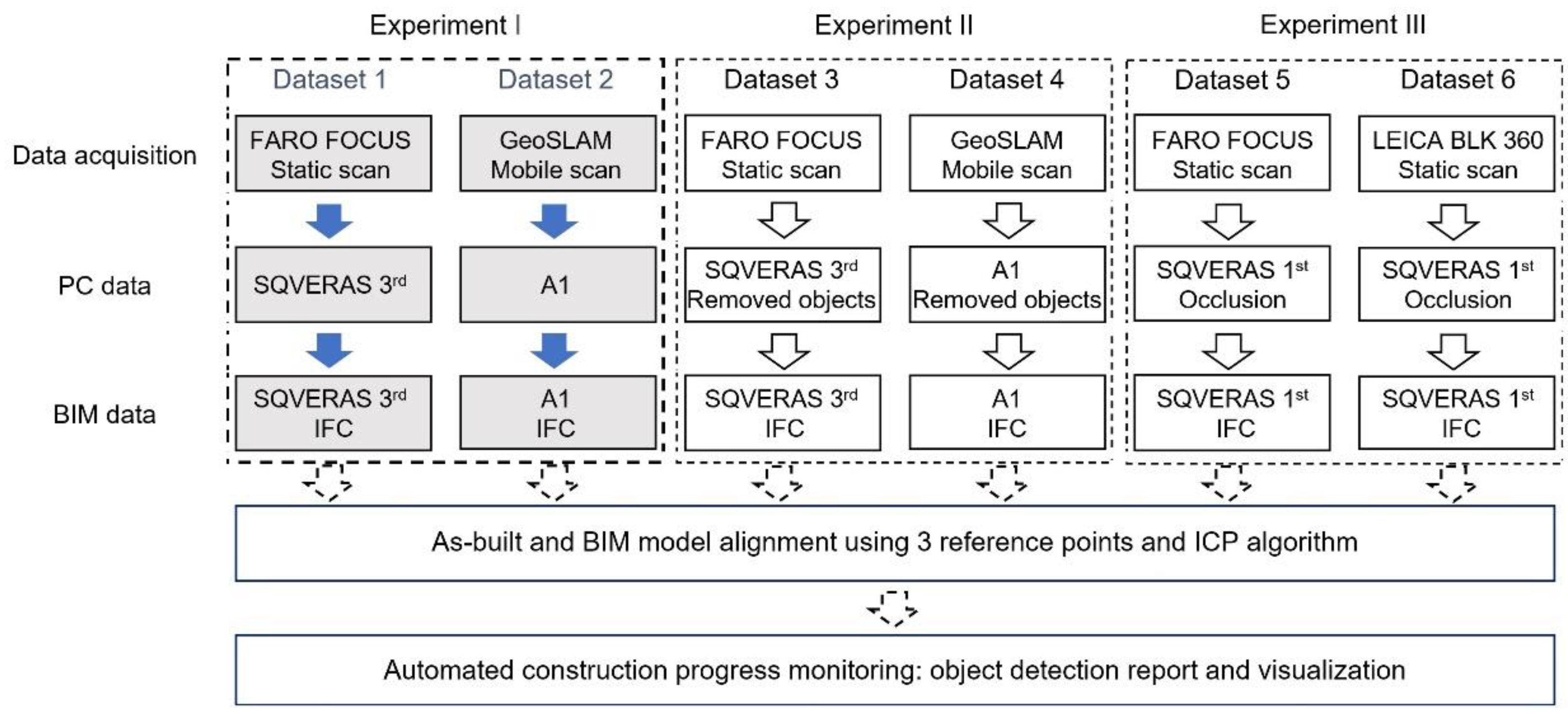
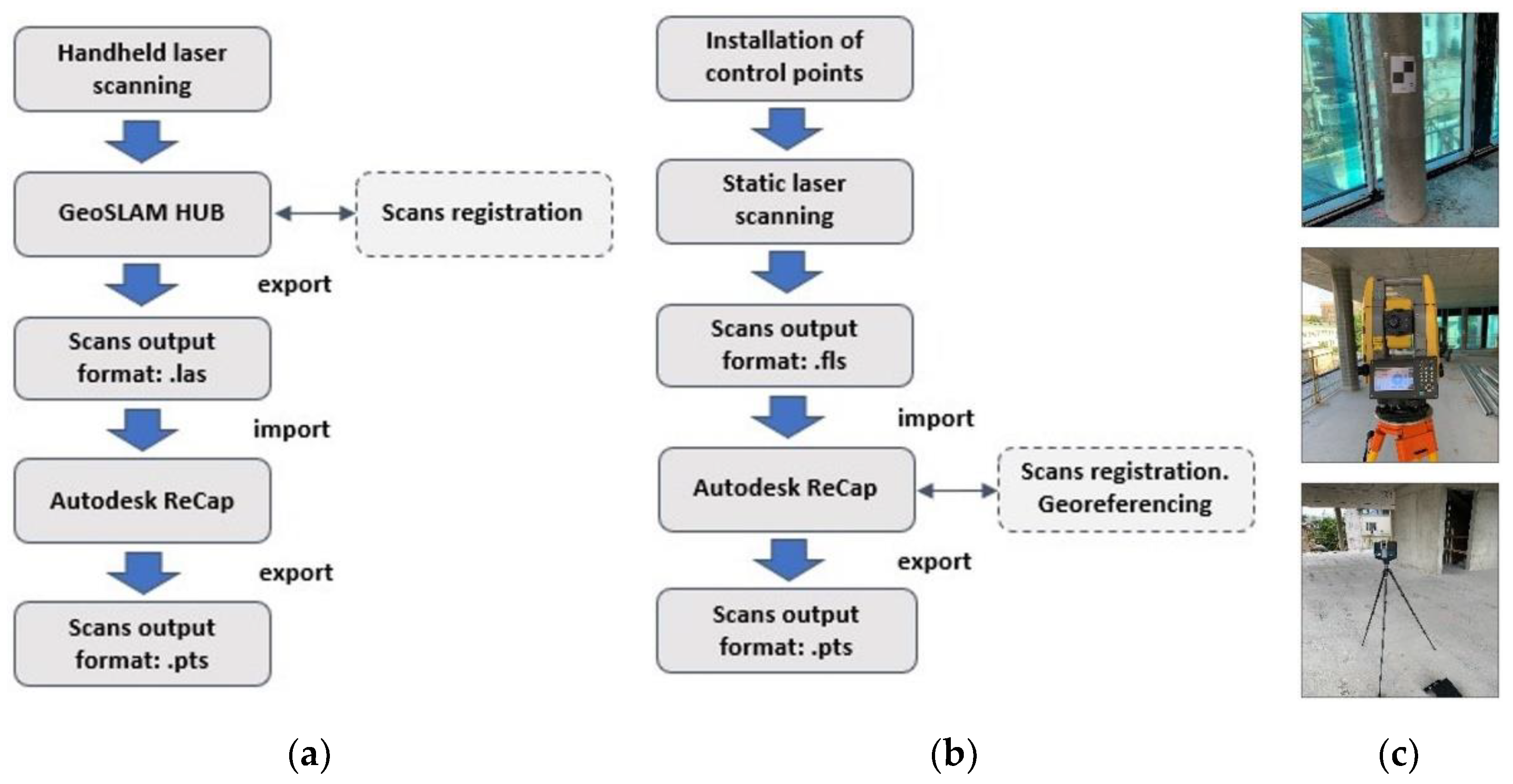
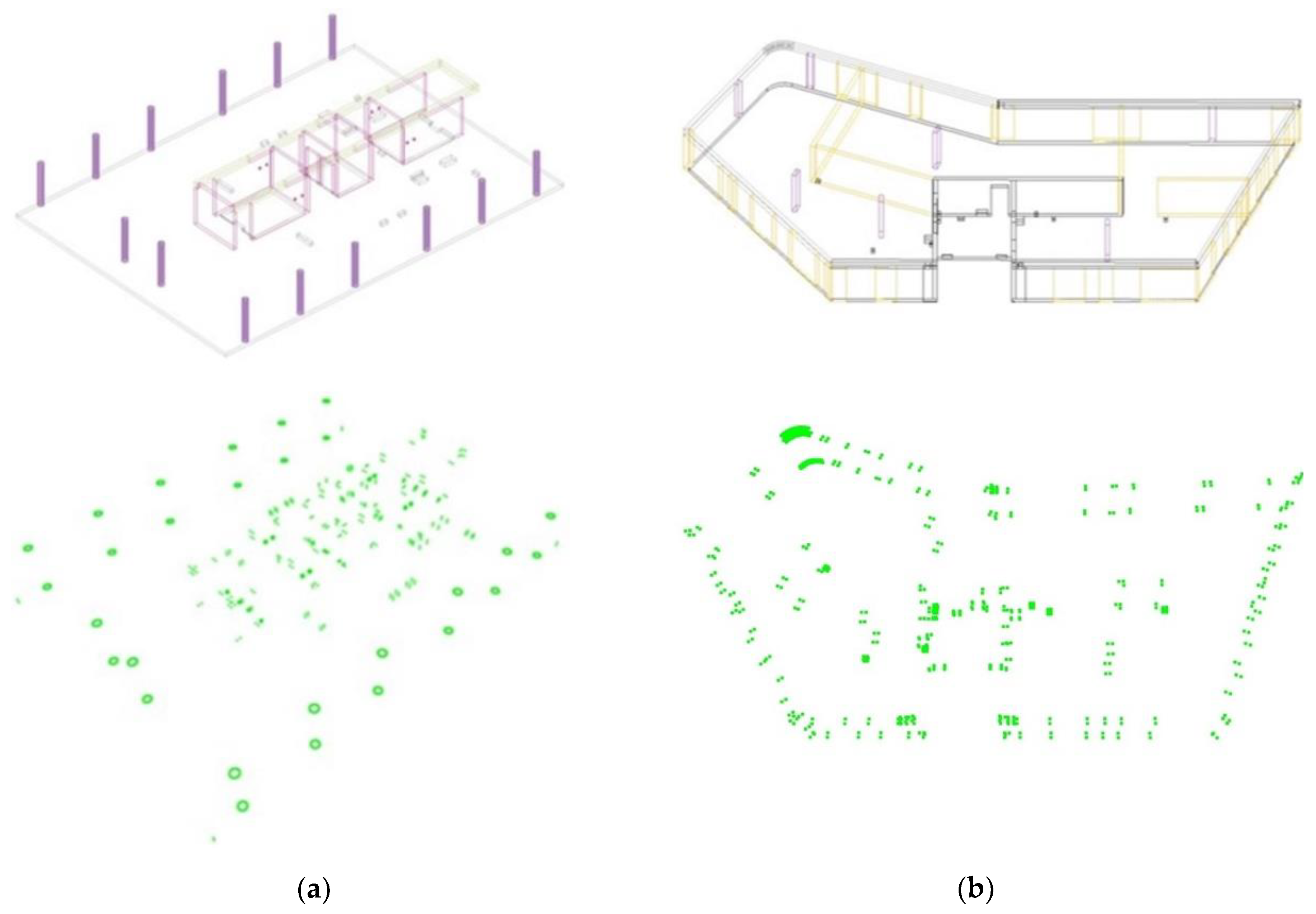
3.1. Data Description
3.2. IFC and Point Cloud Data Alignment
3.2.1. IFC Data Extraction
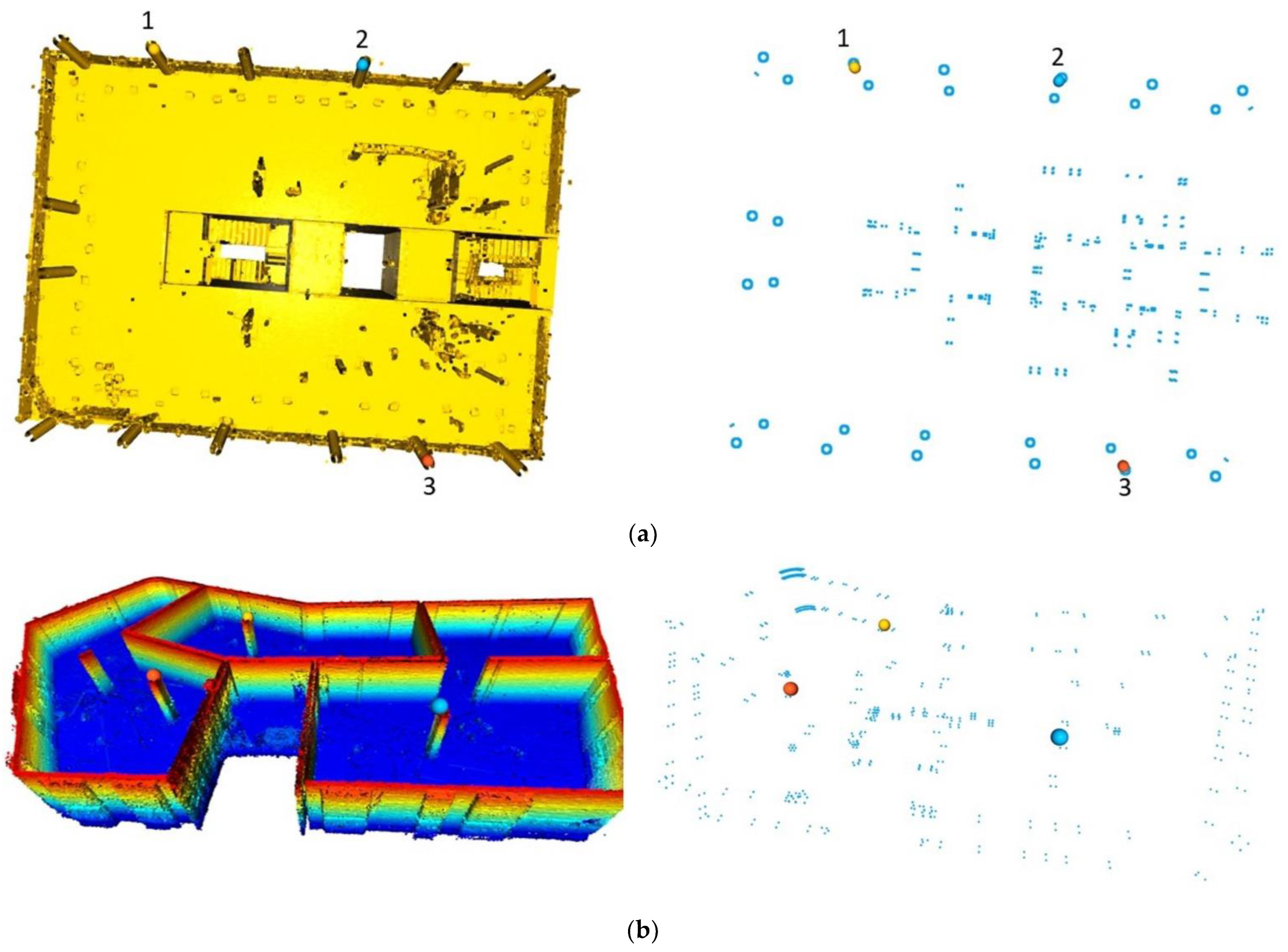
3.2.2. Transformation Estimation Using Three Points of Reference
3.2.3. ICP Point-to-Point Alignment
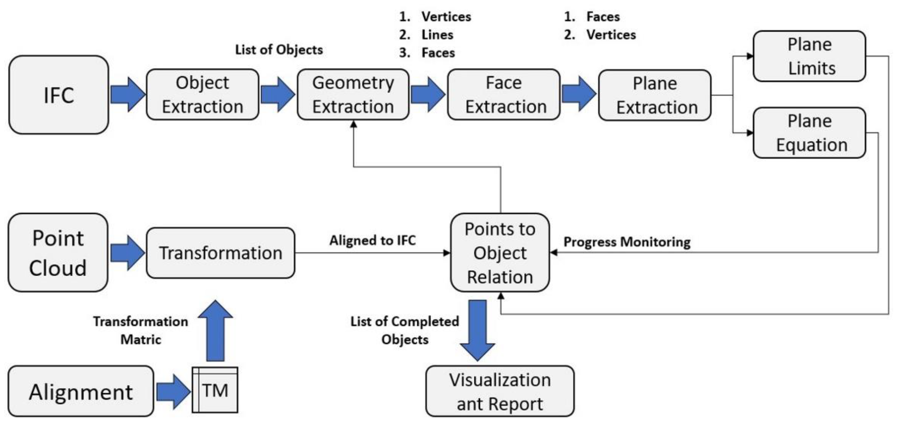
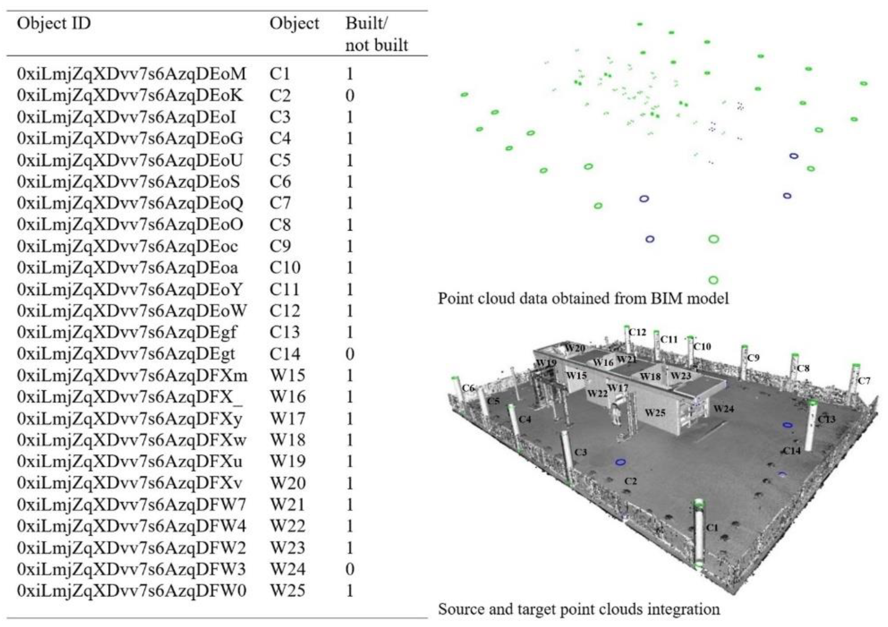
3.3. As-Built vs. IFC Object Monitoring
- Object extraction: As described before, IFC files contain a structured list of objects that belong to a building. This object extraction task was used to explore the IFC files to produce a list of objects IDs.
- Geometry extraction: Each object in an IFC file consists of three main properties: (1) vertices, (2) lines, and (3) faces. The geometry extraction process allowed us to extract these properties.
- Face extraction: IFC files provide face information for each element as a relationship between vertices. As a result, we only extracted face and vertex information in this process.
- Plane extraction: Since we were working with 3D information, this module allowed us to know which plane, namely, or that each face belonged to. This was undertaken by looking at the axis where the plane extended further.
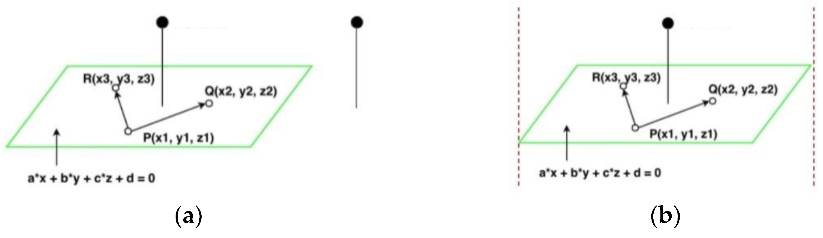
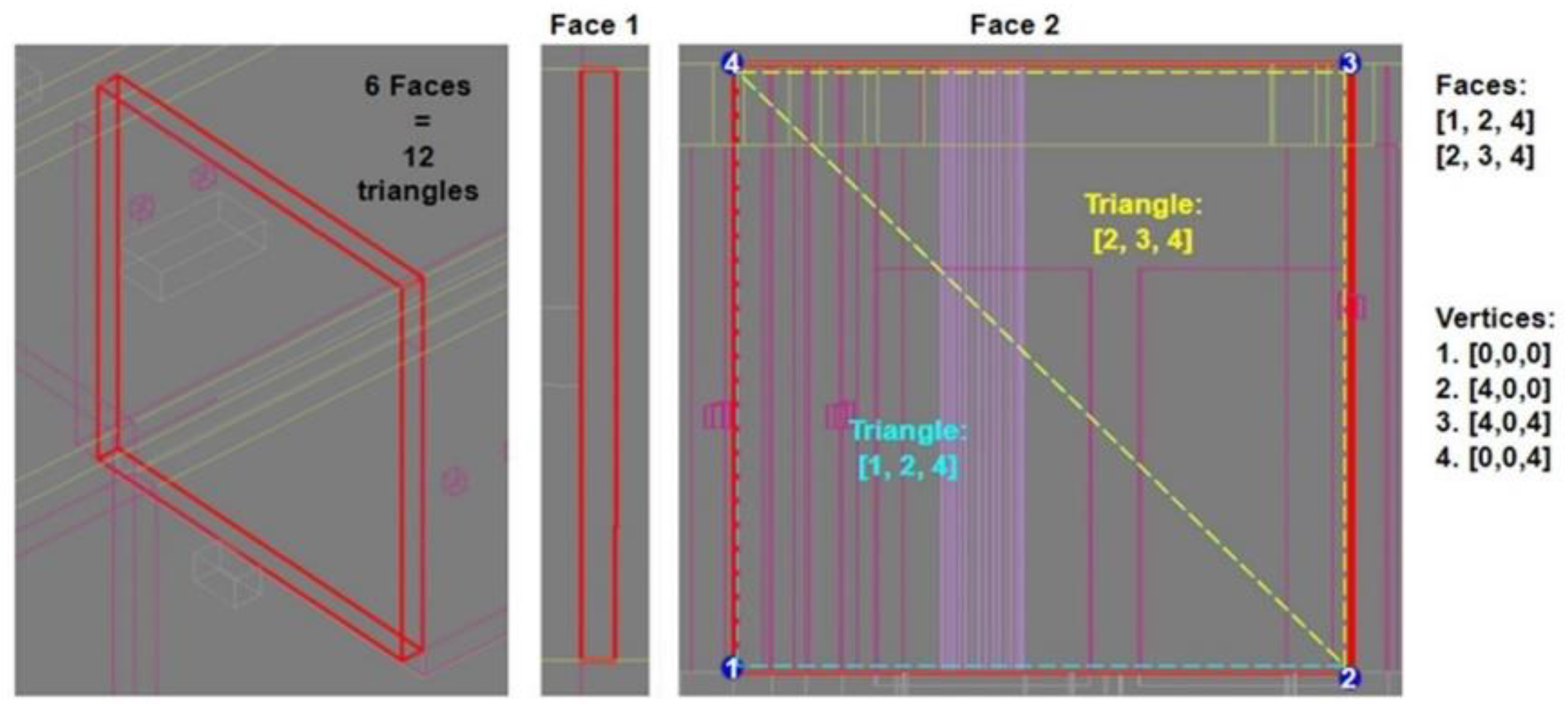
- Plane equation: The methodology we adopted to verify that an object was complete in IFC using point cloud data was to compare how many points were close to the faces of each object. This task is called point-to-plane distance estimation, and to perform such a task, we first need to calculate the face plane equation. In IFC files, the object faces are represented as mesh triangles, which is convenient since we only need three points to calculate the equation of the plane:ax + by + cz + d = 0
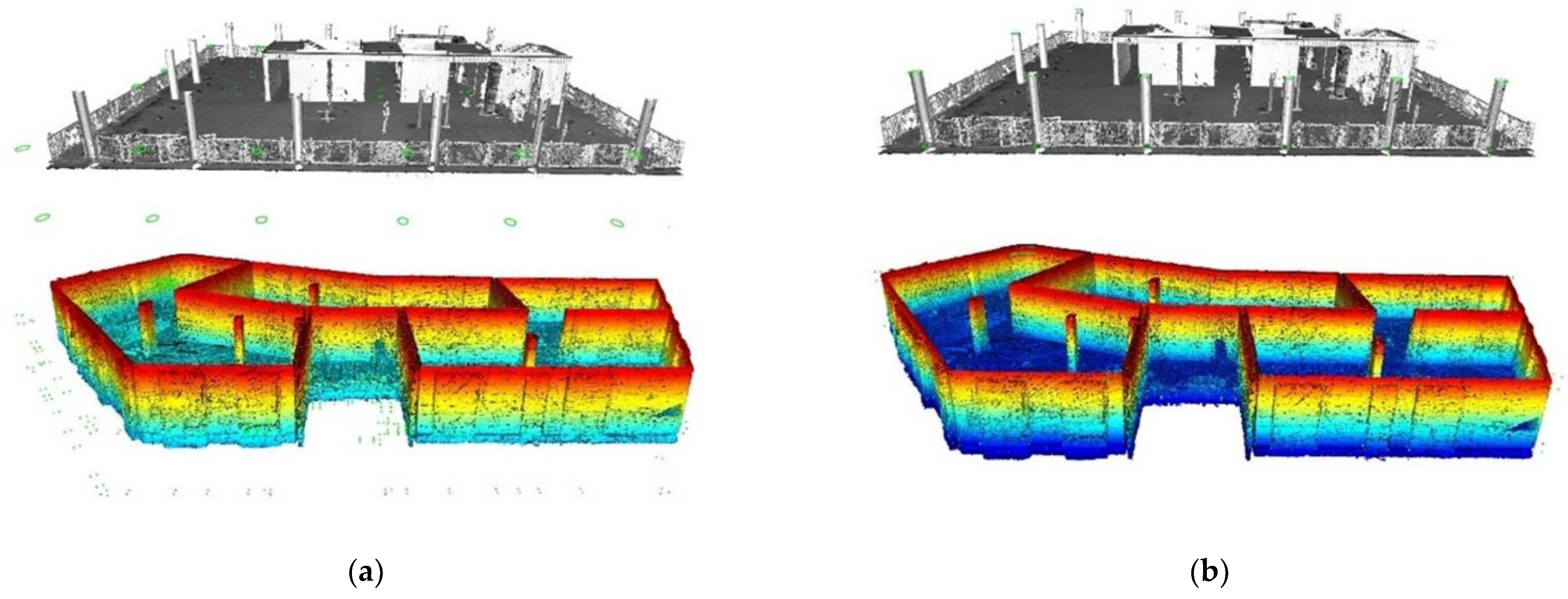
- Plane limits: Since we used the equation of the plane to calculate the distance of a point-to-the plane, this solution calculates the distance to all points, even if they do not belong to the specific limits of the plane, as shown in Figure 7a. This process allowed us to discard those points that were located outside the limits of the current plane (see Figure 7b).
- Point to object relation: Each object was explored and analyzed individually face by face. For each face, the calculation of the plane to point distance estimation was conducted. A point is associated with a face when its distance to the face is less than a threshold. The first output of this module was a list of faces and the number of points related with each face for each object. The final output was a list of objects marked as completed and not completed.
3.4. Optimization
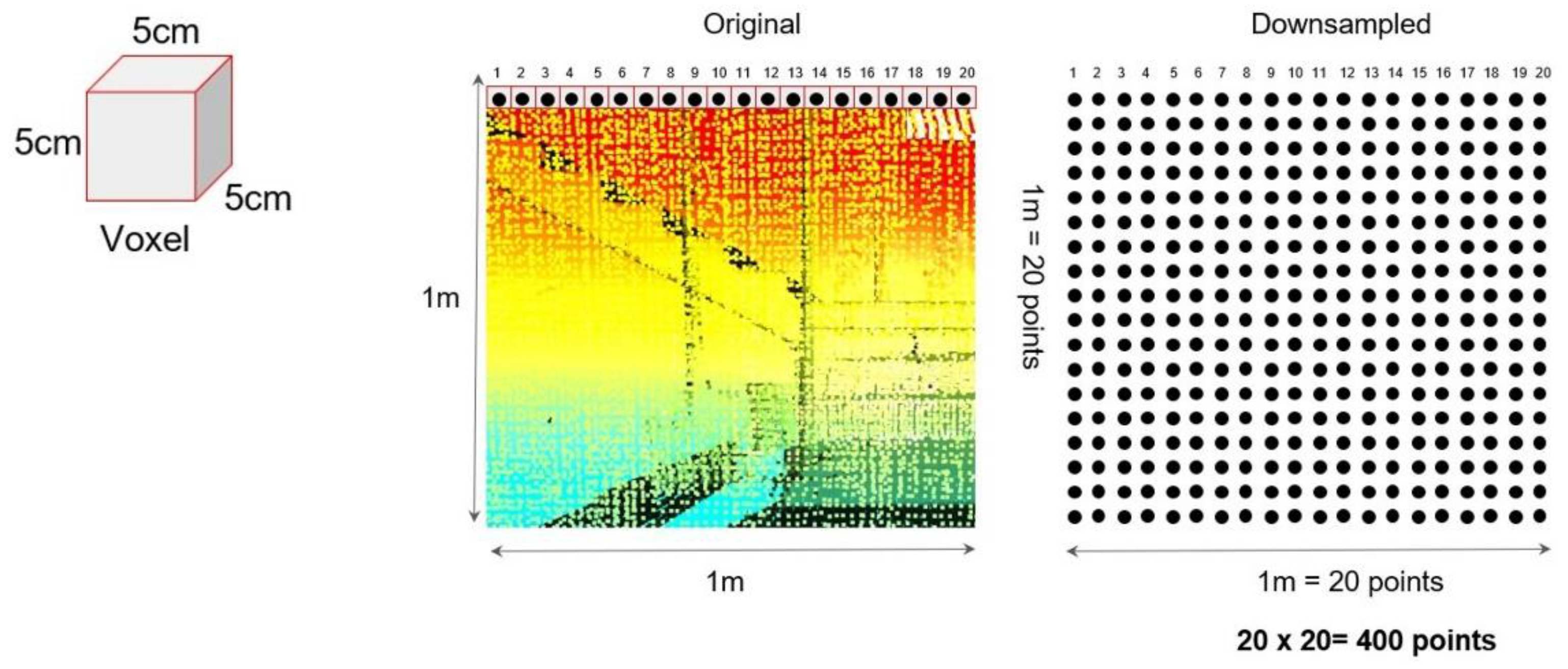
3.4.1. Downsampling
3.4.2. Exploration of One Triangle per Face
4. Results and Discussion
4.1. Alignment
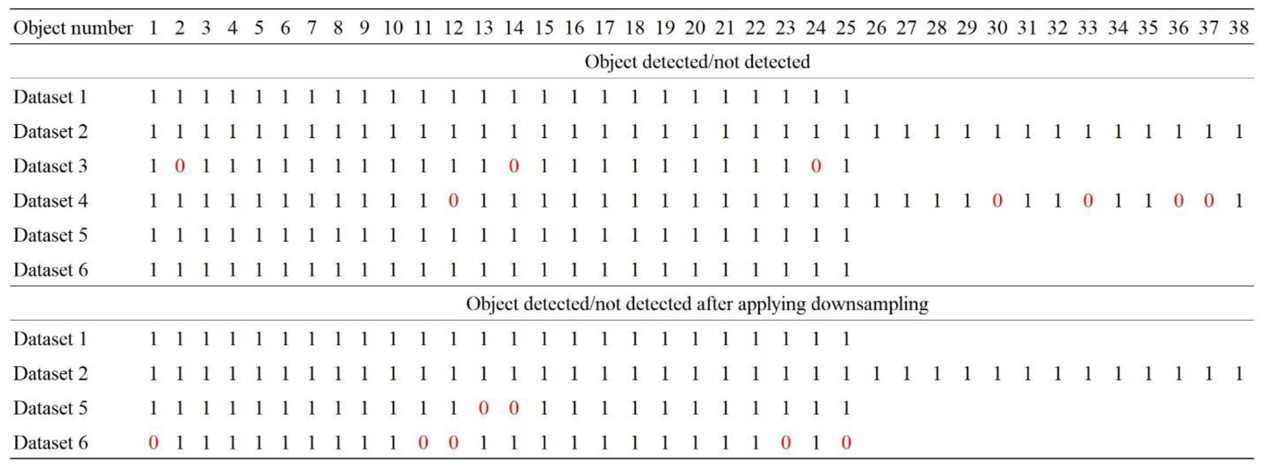
4.2. Evaluation of Object Detection
4.2.1. Removed Objects
4.2.2. Noise Level and Occlusion
4.2.3. Downsampled
4.3. Visualization and Report
5. Conclusions and Future Directions
Author Contributions
Funding
Data Availability Statement
Acknowledgments
Conflicts of Interest
References
- Lavikka, R.; Seppanen, O.; Peltokorpi, A.; Lehtovaara, J. Fostering process innovations in construction through industry–university consortium. Constr. Innov. 2020, 20, 569–586. [Google Scholar] [CrossRef]
- Alizadehsalehi, S.; Yitmen, I. A Concept for Automated Construction Progress Monitoring: Technologies Adoption for Benchmarking Project Performance Control. Arab. J. Sci. Eng. 2019, 44, 4993–5008. [Google Scholar] [CrossRef]
- Kim, C.; Son, H.; Kim, C. Automated Construction Progress Measurement Using A 4D Building Information Model And 3D Data. Autom. Constr. 2013, 31, 75–82. [Google Scholar] [CrossRef]
- Navon, R. Research in Automated Measurement of Project Performance Indicators. Autom. Constr. 2007, 16, 176–188. [Google Scholar] [CrossRef]
- Turkan, Y.; Bosché, F.; Haas, C.; Haas, R. Tracking Secondary and Temporary Concrete Construction Objects Using 3D Imaging Technologies. Comput. Civ. Eng. 2013, 14, 145–167. [Google Scholar] [CrossRef]
- Jadidi, H.; Ravanshadnia, M.; Alipour, M. Visualization of As-Built Progress Data Using Constructionsite Photographs: Two Case Studies. Proc. Int. Symp. Autom. Robot. Constr. (IAARC) 2014, 31, 706–713. [Google Scholar] [CrossRef] [Green Version]
- Bosché, F.; Ahmed, M.; Turkan, Y.; Haas, C.; Haas, R. The Value of Integrating Scan-To-BIM And Scan-Vs-BIM Techniques For Construction Monitoring Using Laser Scanning And BIM: The Case Of Cylindrical MEP Components. Autom. Constr. 2015, 49, 201–213. [Google Scholar] [CrossRef]
- Son, H.; Bosché, F.; Kim, C. As-Built Data Acquisition And Its Use In Production Monitoring And Automated Layout Of Civil Infrastructure: A Survey. Adv. Eng. Inform. 2015, 29, 172–183. [Google Scholar] [CrossRef]
- Hannan Qureshi, A.; Alaloul, W.; Wing, W.; Saad, S.; Ammad, S.; Musarat, M. Factors Impacting the Implementation Process of Automated Construction Progress Monitoring. Ain Shams Eng. J. 2022, 13, 101808. [Google Scholar] [CrossRef]
- Carrera-Hernández, J.; Levresse, G.; Lacan, P. Is UAV-SfM Surveying Ready to Replace Traditional Surveying Techniques? Int. J. Remote Sens. 2020, 41, 4820–4837. [Google Scholar] [CrossRef]
- Abd-Elmaaboud, A.; El-Tokhey, M.; Ragheb, A.; Mogahed, Y. Comparative assessment of terrestrial laser scanner against traditional surveying methods. Int. J. Eng. Appl. Sci. 2019, 6, 79–84. [Google Scholar]
- Giel, B.; Issa, R. Using Laser Scanning to Access the Accuracy of As-Built BIM. In Proceedings of the 2011 ASCE International Workshop on Computing in Civil Engineering, Miami, FL, USA, 19–22 June 2011; pp. 665–672. [Google Scholar] [CrossRef]
- Martinez, J.; Albeaino, G.; Gheisari, M.; Volkmann, W.; Alarcón, L. UAS Point Cloud Accuracy Assessment Using Structure from Motion–Based Photogrammetry and PPK Georeferencing Technique for Building Surveying Applications. J. Comput. Civ. Eng. 2021, 35, 05020004. [Google Scholar] [CrossRef]
- Dai, F.; Lu, M. Assessing the Accuracy of Applying Photogrammetry to Take Geometric Measurements on Building Products. J. Constr. Eng. Manag. 2010, 136, 242–250. [Google Scholar] [CrossRef]
- El-Din Fawzy, H. 3D laser scanning and close-range photogrammetry for buildings documentation: A hybrid technique towards a better accuracy. Alex. Eng. J. 2019, 58, 1191–1204. [Google Scholar] [CrossRef]
- KORUMAZ, S. Terrestrial Laser Scanning with Potentials and Limitations for Archaeological Documentation: A Case Study of the Çatalhöyük. Adv. LiDAR 2021, 1, 32–38. [Google Scholar]
- Bauwens, S.; Bartholomeus, H.; Calders, K.; Lejeune, P. Forest Inventory with Terrestrial LiDAR: A Comparison of Static and Hand-Held Mobile Laser Scanning. Forests 2016, 7, 127. [Google Scholar] [CrossRef] [Green Version]
- Thomson, C.; Apostolopoulos, G.; Backes, D.; Boehm, J. Mobile Laser Scanning for Indoor Modelling. ISPRS Ann. Photogramm. Remote Sens. Spat. Inf. Sci. 2013, II-5/W2, 289–293. [Google Scholar] [CrossRef] [Green Version]
- Trzeciak, M.; Brilakis, I. Comparison of accuracy and density of static and mobile laser scanners. In Proceedings of the 2021 European Conference on Computing in Construction, Rhodes, Greece, 25–27 July 2021. [Google Scholar] [CrossRef]
- Lehtola, V.; Kaartinen, H.; Nüchter, A.; Kaijaluoto, R.; Kukko, A.; Litkey, P.; Honkavaara, E.; Rosnell, T.; Vaaja, M.; Virtanen, J.; et al. Comparison of the Selected State-Of-The-Art 3D Indoor Scanning and Point Cloud Generation Methods. Remote Sens. 2017, 9, 796. [Google Scholar] [CrossRef] [Green Version]
- Wang, B.; Yin, C.; Luo, H.; Cheng, J.; Wang, Q. Fully automated generation of parametric BIM for MEP scenes based on terrestrial laser scanning data. Autom. Constr. 2021, 125, 103615. [Google Scholar] [CrossRef]
- Tzedaki, V.; Kamara, J. Capturing As-Built Information for a BIM Environment Using 3D Laser Scanner: A Process Model. AEI 2013, 2013, 485–494. [Google Scholar] [CrossRef]
- Zhang, C.; Arditi, D. Automated progress control using laser scanning technology. Autom. Constr. 2013, 36, 108–116. [Google Scholar] [CrossRef]
- Turkan, Y.; Bosche, F.; Haas, C.; Hass, R. Automated Progress Tracking of Erection of Concrete Structures. In Proceedings of the Annual Conference of the Canadian Society for Civil Engineering, Ottawa, ON, USA, 14–17 June 2011. [Google Scholar]
- Noardo, F.; Wu, T.; Arroyo Ohori, K.; Krijnen, T.; Stoter, J. IFC models for semi-automating common planning checks for building permits. Autom. Constr. 2022, 134, 104097. [Google Scholar] [CrossRef]
- Koo, B.; Shin, B. Applying novelty detection to identify model element to IFC class misclassifications on architectural and infrastructure Building Information Models. J. Comput. Des. Eng. 2018, 5, 391–400. [Google Scholar] [CrossRef]
- Asadi, K.; Ramshankar, H.; Noghabaei, M.; Han, K. Real-Time Image Localization and Registration with BIM Using Perspective Alignment for Indoor Monitoring of Construction. J. Comput. Civ. Eng. 2019, 33, 04019031. [Google Scholar] [CrossRef]
- Chen, J.; Li, S.; Lu, W. Align to locate: Registering photogrammetric point clouds to BIM for robust indoor localization. Build. Environ. 2022, 209, 108675. [Google Scholar] [CrossRef]
- Soilán, M.; Justo, A.; Sánchez-Rodríguez, A.; Riveiro, B. 3D Point Cloud to BIM: Semi-Automated Framework to Define IFC Alignment Entities from MLS-Acquired LiDAR Data of Highway Roads. Remote Sens. 2020, 12, 2301. [Google Scholar] [CrossRef]
- Huang, R.; Xu, Y.; Yao, W.; Hoegner, L.; Stilla, U. Robust global registration of point clouds by closed-form solution in the frequency domain. ISPRS J. Photogramm. Remote Sens. 2021, 171, 310–329. [Google Scholar] [CrossRef]
- Fan, L.; Atkinson, P. Accuracy of Digital Elevation Models Derived From Terrestrial Laser Scanning Data. IEEE Geosci. Remote Sens. Lett. 2015, 12, 1923–1927. [Google Scholar] [CrossRef]
- Meyer, T.; Brunn, A.; Stilla, U. Change detection for indoor construction progress monitoring based on BIM, point clouds and uncertainties. Autom. Constr. 2022, 141, 104442. [Google Scholar] [CrossRef]
- Pexman, K.; Lichti, D.; Dawson, P. Automated Storey Separation and Door and Window Extraction for Building Models from Complete Laser Scans. Remote Sens. 2021, 13, 3384. [Google Scholar] [CrossRef]
- Maalek, R.; Lichti, D.; Ruwanpura, J. Robust Segmentation of Planar and Linear Features of Terrestrial Laser Scanner Point Clouds Acquired from Construction Sites. Sensors 2018, 18, 819. [Google Scholar] [CrossRef]
- Fontana, S.; Cattaneo, D.; Ballardini, A.; Vaghi, M.; Sorrenti, D. A benchmark for point clouds registration algorithms. Robot. Auton. Syst. 2021, 140, 103734. [Google Scholar] [CrossRef]
- Ge, X. Automatic markerless registration of point clouds with semantic-keypoint-based 4-points congruent sets. ISPRS J. Photogramm. Remote Sens. 2017, 130, 344–357. [Google Scholar] [CrossRef] [Green Version]
- Liu, W.; Sun, W.; Wang, S.; Liu, Y. Coarse registration of point clouds with low overlap rate on feature regions. Signal Process. Image Commun. 2021, 98, 116428. [Google Scholar] [CrossRef]
- Masood, M.; Aikala, A.; Seppänen, O.; Singh, V. Multi-Building Extraction and Alignment for As-Built Point Clouds: A Case Study with Crane Cameras. Front. Built Environ. 2020, 6, 581295. [Google Scholar] [CrossRef]
- Zhang, J.; Yao, Y.; Deng, B. Fast and Robust Iterative Closest Point. IEEE Trans. Pattern Anal. Mach. Intell. 2021, 44, 1. [Google Scholar] [CrossRef]
- Bouaziz, S.; Tagliasacchi, A.; Pauly, M. Sparse Iterative Closest Point. Comput. Graph. Forum 2013, 32, 113–123. [Google Scholar] [CrossRef] [Green Version]
- Mavridis, P.; Andreadis, A.; Papaioannou, G. Efficient Sparse ICP. Comput. Aided Geom. Des. 2015, 35, 16–26. [Google Scholar] [CrossRef]
- Chetverikov, D.; Stepanov, D.; Krsek, P. Robust Euclidean alignment of 3D point sets: The trimmed iterative closest point algorithm. Image Vis. Comput. 2005, 23, 299–309. [Google Scholar] [CrossRef]
- Kaiser, T.; Clemen, C.; Maas, H. Automatic co-registration of photogrammetric point clouds with digital building models. Autom. Constr. 2022, 134, 104098. [Google Scholar] [CrossRef]
- Bosché, F. Plane-based registration of construction laser scans with 3D/4D building models. Adv. Eng. Inform. 2012, 26, 90–102. [Google Scholar] [CrossRef]
- Bueno, M.; Bosché, F.; González-Jorge, H.; Martínez-Sánchez, J.; Arias, P. 4-Plane congruent sets for automatic registration of as-is 3D point clouds with 3D BIM models. Autom. Constr. 2018, 89, 120–134. [Google Scholar] [CrossRef]
- Turkan, Y.; Bosche, F.; Haas, C.; Haas, R. Automated progress tracking using 4D schedule and 3D sensing technologies. Autom. Constr. 2012, 22, 414–421. [Google Scholar] [CrossRef]
- Golparvar-Fard, M.; Peña-Mora, F.; Savarese, S. Automated Progress Monitoring Using Unordered Daily Construction Photographs and IFC-Based Building Information Models. J. Comput. Civ. Eng. 2015, 29, 04014025. [Google Scholar] [CrossRef]
- Pučko, Z.; Šuman, N.; Rebolj, D. Automated continuous construction progress monitoring using multiple workplace real time 3D scans. Adv. Eng. Inform. 2018, 38, 27–40. [Google Scholar] [CrossRef]
- Mahami, H.; Nasirzadeh, F.; Hosseininaveh Ahmadabadian, A.; Nahavandi, S. Automated Progress Controlling and Monitoring Using Daily Site Images and Building Information Modelling. Buildings 2019, 9, 70. [Google Scholar] [CrossRef] [Green Version]
- Wang, Q.; Guo, J.; Kim, M. An Application Oriented Scan-to-BIM Framework. Remote Sens. 2019, 11, 365. [Google Scholar] [CrossRef] [Green Version]
- Braun, A.; Tuttas, S.; Borrmann, A.; Stilla, U. Improving progress monitoring by fusing point clouds, semantic data and computer vision. Autom. Constr. 2020, 116, 103210. [Google Scholar] [CrossRef]
- Romero-Jarén, R.; Arranz, J. Automatic segmentation and classification of BIM elements from point clouds. Autom. Constr. 2021, 124, 103576. [Google Scholar] [CrossRef]
- Bassier, M.; Klein, R.; Van Genechten, B.; Vergauwen, M. IFC walls reconstruction from unstructured point clouds. ISPRS Ann. Photogramm. Remote Sens. Spat. Inf. Sci. 2018, IV-2, 33–39. [Google Scholar] [CrossRef]
- Rausch, C.; Haas, C. Automated shape and pose updating of building information model elements from 3D point clouds. Autom. Constr. 2021, 124, 103561. [Google Scholar] [CrossRef]
- Yang, L.; Cheng, J.; Wang, Q. Semi-automated generation of parametric BIM for steel structures based on terrestrial laser scanning data. Autom. Constr. 2020, 112, 103037. [Google Scholar] [CrossRef]
- Krijnen, T.; Beetz, J. An IFC schema extension and binary serialization format to efficiently integrate point cloud data into building models. Adv. Eng. Inform. 2017, 33, 473–490. [Google Scholar] [CrossRef]


| Dataset No. | Description |
|---|---|
| Dataset 1 | Consists of as-built data obtained from the third floor of the office building and the corresponding IFC-based BIM model. As-built data was obtained using a FARO Focus S70 static laser scanner in a clean environment. The resulting point cloud was georeferenced to the global coordinate system. |
| Dataset 2 | Consists of as-built data obtained from the residential building and the corresponding IFC-based BIM model. As-built data was obtained using a ZEB-GO mobile laser scanner in a clean environment. |
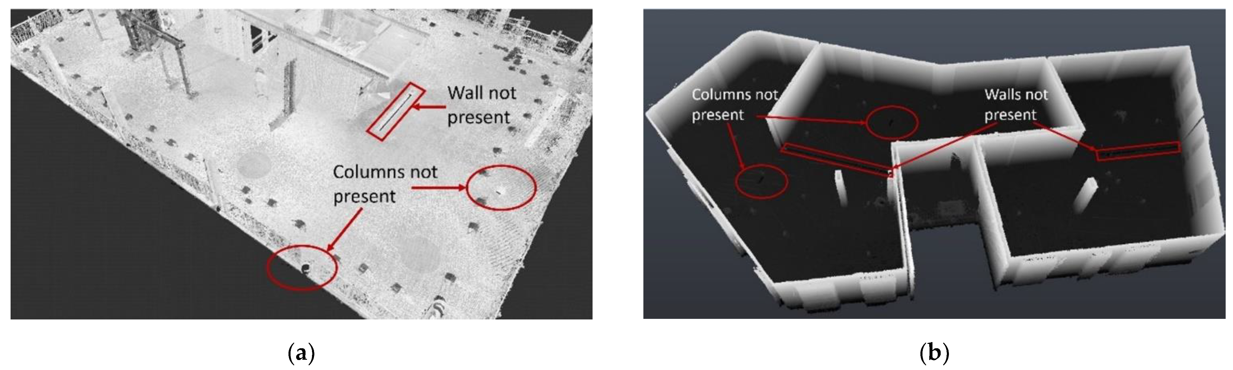
| Dataset 3 | Consists of modified data from Dataset 1. A wall and two columns were removed from the point cloud model. The corresponding IFC-based BIM model was not modified. |
| Dataset 4 | Consists of modified data from Dataset 2. Two walls and two columns were removed from the point cloud model. The corresponding IFC-based BIM model was not modified. |
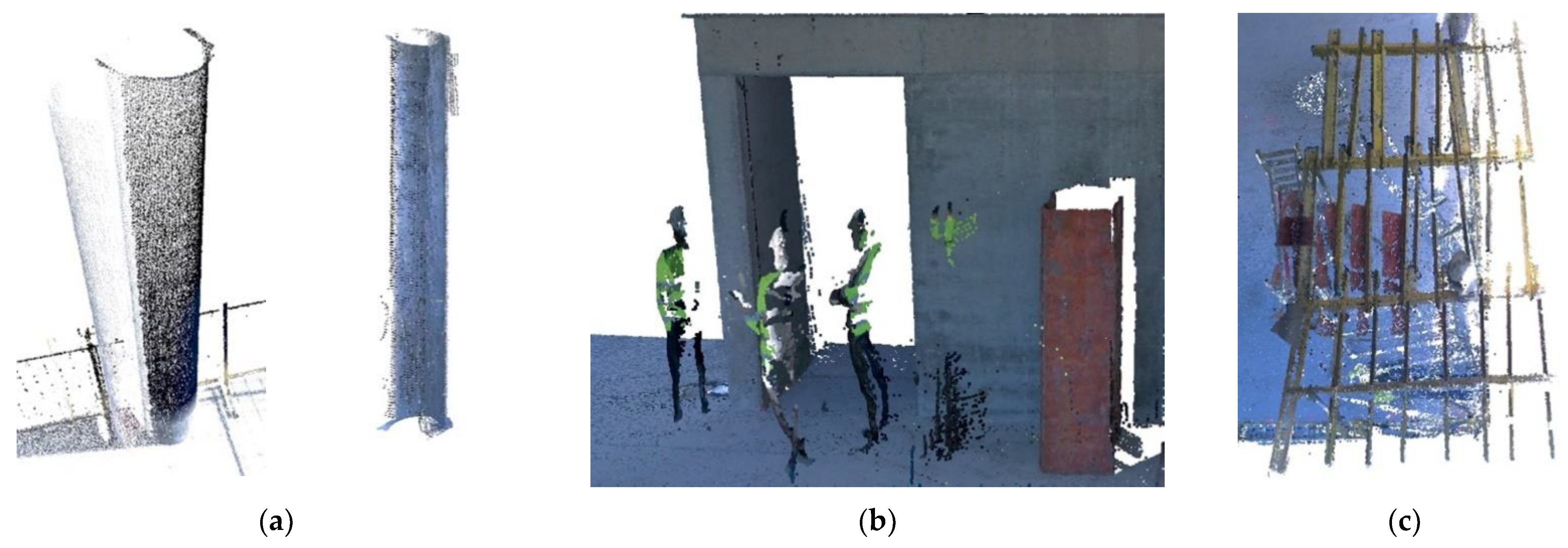
| Dataset 5 | Consists of as-built data obtained from the first floor of the office building and the corresponding IFC-based BIM model. As-built data was obtained using a FARO Focus S70 static laser scanner in an occluded environment. Unnecessary points in the point cloud affected by noise were not removed. |
| Dataset 6 | Consists of as-built data obtained from the first floor of the office building and the corresponding IFC-based BIM model. As-built data was obtained using a Leica BLK 360 static laser scanner in an occluded environment. Unnecessary points in the point cloud affected by noise were not removed. |
| Device | Type | Distance Accuracy | Scanning Range (Meters) | Scanning Speed (Points/Second) |
|---|---|---|---|---|
| FARO Focus S70 laser scanner | Terrestrial | 1 mm | 70 | 1,000,000 |
| ZEB-GO handheld laser scanner and ZEB-DL2600 data logger | Handheld | 10–30 mm | 30 | 43,000 |
| Leica BLK360 laser scanner | Terrestrial | 4 mm at 10 m | 60 | 360,000 |
| 7 mm at 20 m |
| Point Cloud Data | Date | Average Population (Points/m3) | Number of Points | File Size (MB) |
|---|---|---|---|---|
| SQVERAS 3rd floor obtained using Faro laser scanner | 2 July 2019 | 1438.78 | 9,451,351 | 758 |
| A1 obtained using ZEB-GO laser scanner | 24 December 2021 | 521.48 | 12,510,712 | 677 |
| SQVERAS 1st floor obtained using Faro laser scanner | 2 July 2019 | 2211.69 | 13,882,774 | 1007 |
| SQVERAS 1st floor obtained using Leica laser scanner | 4 June 2019 | 726.60 | 12,990,132 | 903 |
| Point Cloud Data | Original PC (Number of Points) | Method Validation | Downsampled PC (Number of Points) | Method Validation |
|---|---|---|---|---|
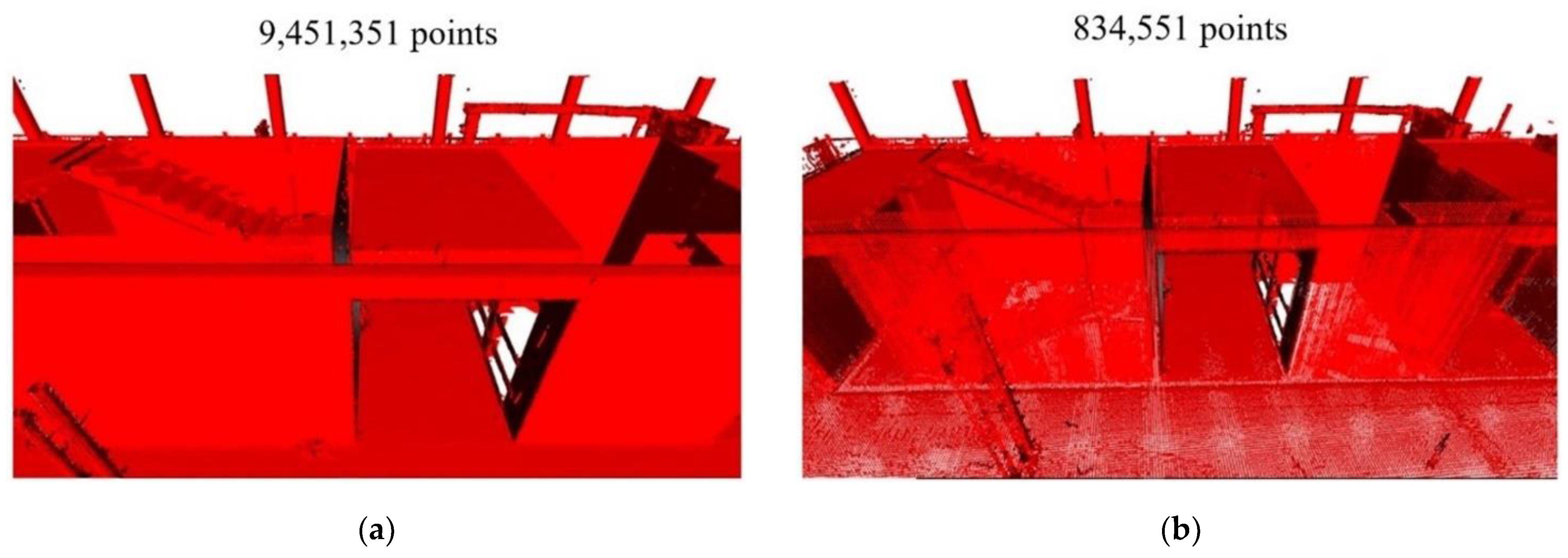
| SQVERAS 3rd floor obtained using a Faro laser scanner | 9,451,351 | All objects detected | 834,551 | All objects detected |
| A1 obtained using a ZEB-GO laser scanner | 12,510,712 | All objects detected | 1,236,999 | All objects detected |
| SQVERAS 1st floor obtained using a Faro laser scanner | 13,882,774 | All objects detected | 641,578 | Not all objects detected |
| SQVERAS 1st floor obtained using a Leica laser scanner | 12,990,132 | All objects detected | 532,111 | Not all objects detected |
Publisher’s Note: MDPI stays neutral with regard to jurisdictional claims in published maps and institutional affiliations. |
© 2022 by the authors. Licensee MDPI, Basel, Switzerland. This article is an open access article distributed under the terms and conditions of the Creative Commons Attribution (CC BY) license (https://creativecommons.org/licenses/by/4.0/).
Share and Cite
Kavaliauskas, P.; Fernandez, J.B.; McGuinness, K.; Jurelionis, A. Automation of Construction Progress Monitoring by Integrating 3D Point Cloud Data with an IFC-Based BIM Model. Buildings 2022, 12, 1754. https://doi.org/10.3390/buildings12101754
Kavaliauskas P, Fernandez JB, McGuinness K, Jurelionis A. Automation of Construction Progress Monitoring by Integrating 3D Point Cloud Data with an IFC-Based BIM Model. Buildings. 2022; 12(10):1754. https://doi.org/10.3390/buildings12101754
Chicago/Turabian StyleKavaliauskas, Paulius, Jaime B. Fernandez, Kevin McGuinness, and Andrius Jurelionis. 2022. "Automation of Construction Progress Monitoring by Integrating 3D Point Cloud Data with an IFC-Based BIM Model" Buildings 12, no. 10: 1754. https://doi.org/10.3390/buildings12101754