Article

A Mesoscopic Viewpoint on Slurry Penetration and Pressure Transfer Mechanisms for Slurry Shield Tunneling

1
School of Resources and Civil Engineering, Northeastern University, Shenyang 110004, China
2
School of Qilu Transportation, Shandong University, Jinan 250002, China
3
School of Civil Engineering, Dalian University of Technology, Dalian 116024, China
*
Author to whom correspondence should be addressed.
Buildings 2022, 12(10), 1744; https://doi.org/10.3390/buildings12101744
Submission received: 26 September 2022 / Revised: 11 October 2022 / Accepted: 12 October 2022 / Published: 19 October 2022

Abstract

:
The penetration characteristics of the slurry and the support pressure transfer mechanisms are critical to the tunnel face stability control during a mechanized excavation. In this paper, numerical calculations coupling computational fluid dynamics (CFD) with the discrete element method (DEM) are carried out to simulate sand column penetration tests considering different particle size ratios. The reasonableness of the numerical model is verified by comparing the variation patterns of the soil permeability coefficients monitored in the numerical tests with the results of existing laboratory tests. The mesoscopic transport characteristics of the slurry particles in the sand soil pores are considered based on numerical tests, while the slurry support effects corresponding to different penetration types are evaluated. Three main basic types of slurry infiltration are observed due to the different ratios of slurry particle size over soil pore size. For the first penetration type, the slurry particles are accumulated and able to form a supporting filter cake. The slurry support is effective because of the significant pressure drop generated on both sides of the filter cake. For the second penetration type, both a filter cake and an infiltration zone are present. A dense filling network is formed between the filter cake and the penetration zone. The third type corresponds to a purely penetration zone. An effective impermeable filling network cannot be formed, and the slurry support effect is not obvious. The development of slurry penetration distance shows an obvious time effect; the farther the penetration distance, the larger the slurry filtration loss, and the worse the transformation effect of slurry support pressure.

1. Introduction

During the excavation process of a mechanized tunnel, the instantaneous stability of the tunnel face is provided by the bentonite slurry or by compressed air in the cutting shield chamber. This phenomenon is more obvious when using a slurry shield. Two fundamental conditions are necessary to satisfy stabilizing the tunnel face: a sufficient face support pressure in the excavation chamber and an efficient pressure transfer of the excess slurry pressure onto the soil skeleton. A large amount of research was carried out on the limit support tunnel face pressure. The first research was the silo wedge model [1] based on the limit equilibrium theory. It has been widely used due to its simplicity. Then, this model was continuously improved to be able to consider more complicated situations [2,3]. Meanwhile, the limit analysis theory [4,5,6,7] has permitted giving a reasonable range of the upper and lower bounds of the limit support pressure in a more rigorous background. This method considers a kinematically admissible velocity field (upper bound) or a statically admissible stress field (lower bound). With the continuous development of the computer performance, the construction of complex velocity fields closer to real ones has permitted improving the accuracy of the tunnel support pressure to a greater extent [8,9]. Considering numerical approaches, it is nowadays the most popular method due to the development of powerful numerical tools allowing for 3D analysis [10,11,12]. Nevertheless, numerical approaches are more computationally expensive than the limit equilibrium or limit analysis ones.
During a tunnel excavation using a slurry shield, the tunnel face is supported by the slurry which is a mixture of bentonite in suspension. The suspension slurry will create a quasi-impervious membrane (filter cake); therefore, the support pressure can be applied to resist the soil pressure and hold the groundwater pore pressure if the soil permeability is relatively low (<1 × 10⁻⁴ m/s) and the percentage of bentonite is enough [13]. However, when the soil has high permeability (>1 × 10⁴ m/s) such as coarse sands and gravels or the parameters (e.g., grading, concentration, etc.) of the slurry are variable, the pressure generated in the excavation chamber may not always be effectively transferred into an effective support pressure acting on the soil skeleton. The slurry support technology in a slurry shield originated from the diaphragm wall technology [14]. Therefore, the slurry support mechanism on the excavation face has received extensive attention in past research [15,16,17,18]. The first attempts to analyze the interaction between slurry and soil were conducted by Morgenstern and Amir-Tahmasseb [14] for the purposes of open trench stabilization. However, the authors did not establish any connection between the support mechanism and the support effect. Their theory expects that all the excess slurry pressure is transferred to the soil skeleton. Müller-Kirchenbauer [15] found that the slurry penetration behavior is determined by the soil’s grain size distribution and the slurry pressure gradient along the entire infiltration path (stagnation gradient). Based on their results, two forms of slurry and soil interaction were proposed: type I is a filter cake on the excavation surface, and type II is an infiltrated zone through the soil pores without filter cake. For type II, they stated that the slurry penetration distance was determined by the stagnation gradient and the excess pressure of the slurry. Based on this research, Kilchert and Karstedt [16] further divided the form of slurry and soil interaction into three types. In addition to the two types mentioned above, there are also combinations of the former two types, which have permitted completing the classic theoretical framework of slurry and soil interaction.
In existing theoretical research, the study of slurry and soil interaction is almost based on the porous media seepage theory, and there is no detailed analysis of the interaction form of slurry particles and soil particles at the mesoscale. Therefore, the blocking effect of porous media on fluid flow is described by a single variable, the permeability coefficient, which is usually obtained through laboratory tests [19,20]. The slurry stagnation gradient is a key indicator for evaluating the penetration behavior using laboratory tests. The dependency of the stagnation gradient on the characteristic grain size (d10) and the slurry yield point was derived from experiments [21]. The impact of key slurry parameters (e.g., bentonite concentration, clay content, viscosity, and density) on the filter cake quality was also the focus of researchers at the same time [22,23,24,25,26]. Min et al. [27] suggested a methodology to predict which of the three types (filter cake, infiltration zone, and mix between filter cake and infiltrated zone) occurs in highly permeable sands. The comparison between the average soil pore sizes (Dp) with the soil particles size suspended in slurry is the main parameter of this methodology. In laboratory sand column tests [27], the pore water pressure changes during the slurry infiltration process, and the slurry accumulation can be clearly observed at the sand column surface. However, the mesoscopic transport patterns of the slurry particles inside the sand column and the mechanism of interaction with soil particles could not be observed.
It is worth noting that for a tunnel excavation using a slurry shield, no matter what type of pressure transfer mechanism is formed at the excavation surface, the continuous rotation of the shield cutter induces cyclic mechanisms due to the cycles of excavation/support pressure. Slurry infiltration is not an instantaneous process but an ongoing one. The residual slurry particles in the ground after the cutting tools’ passage will influence the subsequent slurry infiltration behavior. The slurry penetration behavior will then be different for different penetration stages. This will influence the slurry support effect. Therefore, it is necessary to consider the time effect of the pressure transfer mechanisms. Although Krause [28] emphasized the significance of considering the time effect in the pressure transfer mechanism analysis, no in-depth research has been carried out on the slurry infiltration process. Anagnostou and Kovári [29] developed a theoretical model determining the time-dependent slurry penetration depth specifically for slurry shield tunneling. Xu et al. [30] proposed a calculation method for the pore water pressure distribution at the tunnel face based on on-site monitoring data. In all the cases, the model tests or on-site monitoring cannot effectively reflect the microscopic migration of the slurry particles in the soil pores during the different mechanism formation stages. Theoretical analysis [16,29] ignored the development of the slurry penetration and used a constant permeability coefficient. However, numerical methods can effectively reflect the mechanical characteristics of the infiltration zone at different times of the slurry infiltration process, especially the discrete element method which can intuitively reflect the microscopic mechanism of the slurry soil interaction. Zhang et al. [31] studied the formation process of the type I mechanism and the slurry key parameters’ influence on the quality of the filter cake using a CFD-DEM coupling method. However, there is no in-depth analysis of the other types of pressure transfer mechanism that can exist in real projects. The effect of the pressure transfer is not easy to evaluate when the second or third type of pressure transfer mechanism are developed. It is significant to explore the mechanism and effect of slurry support for the stability control of a slurry shield tunnel face when an intact filter cake cannot be formed.
To further study the slurry penetration and support pressure transfer mechanisms in the sand layers, the present study focused on the analysis of the slurry penetration characteristics and on the main control conditions of different penetration types with the help of coupled CFD-DEM simulations using a coarse-grid method. Based on the particle grading relationship between the slurry and the sand, different slurry infiltration types and the corresponding slurry support effects were analyzed. The different filter cake formation stages were analyzed, and the numerical results were compared with the laboratory test results. Finally, the slurry support pressure transfer mechanisms and the support effect under the control of different grading conditions were clarified.

2. Methodology and Theoretical Background

In this study, the discrete element software PFC3D [32] was used for calculations. The numerical method was developed based on the theory of mesoscopic discontinuity mechanics. The medium is composed of a series of spheres or clumps which can simulate different media by giving the spheres or clumps different properties and contact patterns. The method allows calculating a displacement field but can also effectively simulate discontinuous phenomena such as cracking and the separation of particles. To study the microscopic mechanism of slurry particles’ migration in the soil pores intuitively, a slurry–soil interaction model was established using DEM. A coupling between CFD and DEM was originally proposed by Tsuji et al. [33]. It was fully developed and widely used to study multiphase flow problems [34]. This method analyzes the fluid problem by discretizing the continuous fluid into fluid elements and solving the fluid motion equation. FiPy [35] was used in the calculations as a partial differential equation solver based on the finite volume method. By connecting FiPy to the CFD module, DEM and CFD can exchange calculation information during the calculation process.

2.1. Particle Motion Equation

During the DEM calculations, the particles’ movements must satisfy Newton’s second law (Equation (1)) and the momentum conservation law (Equation (2)).
u t = f m e c h + f f l u i d m + g
ω t = M I
where u is the particle velocity; m is the particle mass; f m e c h is the total external force acting on the particle (including the applied external force and the contact force between the particles); f f l u i d is the total force exerted by the fluid on the particles; g is the gravity acceleration; ω is the particle rotation velocity; I is the particle moment of inertia; and M is the moment acting on the particle.
The force exerted by the fluid on the particles f f l u i d (fluid–particle interaction force) consists of two parts: the drag force and the force caused by the fluid pressure gradient. The drag force is calculated based on the fluid element porosity and is distributed according to the overlap ratio of the particles and the fluid element. The fluid drag force [33] on the particle is applied at the particle centroid. The calculation formula is
f d r a g = f 0 ξ χ
where f 0 is the drag force experienced by a single particle, and ξ is the fluid element porosity where the particle is located, which represents the volume ratio of the pore portion in the fluid element other than the particles. ξ-χ is a correction term, which makes the calculation formula suitable for both high porosity and low porosity, supporting a wide range of Reynolds number values. χ is an empirical coefficient considering local porosity, which is related to the Reynolds number.
The drag force experienced by a single particle is equal to
f 0 = ( 1 2 C d ρ f π r 2 | u v | ( u v ) )
where Cd is the drag force coefficient, the empirical value related to the particle Reynolds number is used in the calculation. ρf is the fluid density; r is the particle radius; v is the fluid velocity; and u is the velocity of the particle.
The drag force coefficient is defined as
C d = ( 0.63 + 4.8 R e P ) 2
The empirical coefficient χ is defined as
χ = 3.7 0.65 exp ( ( 1.5 log 10 R e P ) 2 ) 2
where Rep is the particle Reynolds number, which can be expressed as:
R e p = 2 ρ f r | u v | μ f
where μf is the fluid dynamic viscosity coefficient.
Therefore, the total force exerted by the fluid on the particles is
f f l u i d = f d r a g + 4 3 π r 3 ( p ρ f g )
The first term in the above formula is the drag force generated by the fluid on the particles, the second term is the force caused by the fluid pressure gradient.

2.2. Fluid Motion Equation

For the fluid movement, it is considered that the fluid volume is incompressible. Then, the continuity equation (mass conservation equation) and the Navier–Stokes equation (momentum conservation equation) of the fluid can, respectively, be expressed as
ξ t = ( ξ v )
( ξ v ) t = ( ξ v v ) ξ ρ f p ξ ρ f τ + ξ g + f int ρ f
where ξ is the fluid element porosity. t is the calculation time. ▽ is the gradient operator, = ( / x , / y , / z ) . v is the fluid velocity vector. ρf is the fluid density. ▽p is the fluid pressure gradient. τ is the fluid viscous stress tensor. g is the gravity acceleration. fint is the interaction force between the particles and the fluid per unit volume.
The average fluid element volumetric force was used to calculate the interaction force between particles and fluid. The average volumetric force is obtained by summing the fluid drag forces on all particles inside the fluid element and divided by the total fluid element volume.
f int = i = 1 n f 0 i / V
where n represents the total number of particles for a given fluid element. f 0 i is the drag force experienced by a single particle numbered i. V is the volume of a given fluid element.

2.3. Fluid–Solid Coupling

A computational fluid dynamics (CFD) module is implemented in PFC3D. It allows solving some fluid particle interaction problems. This module provides commands and script functions and solves the problem of fluid particle interaction through the volume average-based coarse-grid method. In the coarse-grid method, the equations describing the fluid flow are solved on a set of elements larger than the DEM particles. Additionally, this method can increase calculation efficiency while maintaining calculation accuracy. According to the flow conditions in the fluid element where the particles are located, the fluid force is distributed on each particle. In that way, the fluid–particle interaction force changes smoothly within the actual range of porosity and Reynolds number.
A corresponding volume force is applied by homogenizing the fluid element. The porosity and fluid drag force of each fluid element are calculated from the average value of particle properties. The coupling calculation is realized by periodically exchanging information between the DEM and the fluid solver. In the DEM calculation, it is generally assumed that the fluid element size is larger than the particle size, the fluid properties are piecewise linearly distributed in the fluid element, and the fluid elements are not movable. The porosity of the fluid element is calculated by the amount of overlap between the DEM particles and the fluid element. Because particles will migrate during the process of fluid–solid coupling, and the porosity of the fluid element will also change, the permeability coefficient of solid particles to fluid is calculated by the Kozeny–Carman [36] formula.
k ( ξ ) = { 1 180 ξ 3 ( 1 ξ ) 2 ( 2 r ) 2         ξ 0.7 k ( 0.7 )                                     ξ > 0.7
where r is the radius of the DEM particles. To calculate the permeability coefficient, the upper limit of the porosity is set to 0.7. If the porosity exceeds 0.7, the permeability coefficient is taken as a constant [32].
The CFD module automatically applies a fluid–particle interaction force to the DEM particles. The two-way coupling is achieved by updating the porosity and permeability coefficient in the fluid flow model, and by updating the fluid velocity field in the CFD module. The fluid Equation (9) and Equation (10) are solved on a coarse-grid element set, and the flow velocity is piecewise linearly distributed on the fluid elements. The specific realization process of fluid–solid coupling is shown in Figure 1.

3. Adopted Numerical Model

3.1. Modeling the Slurry Penetration Using CFD-DEM

The most common slurry penetration test is the infiltration sand column test [22,24,27,37] and a common test apparatus is shown in Figure 2. Existing numerical models [31,38] for slurry infiltration are often set up based on indoor test setups so that they can verify the validity by comparing with indoor test results. To study the slurry particles movements in the soil pores, it is necessary to use a numerical model to simulate the infiltration behavior of slurry particles. Generally, there are two ways to characterize the slurry penetration behavior in CFD–DEM calculations: (1) The use of a non-Newtonian fluid model, such as the Bingham model or Herschel–Bulkley models, which usually regard the solid particles and fluid as a unified material. (2) Independently introduce the slurry particles [39] and use a Newtonian fluid model to characterize the viscous contact between fluid and particles [40]. In this research, the effect of the slurry support pressure transfer mechanism under different types of slurry–soil interaction mechanisms is studied. The process of filling the soil pore structure with slurry particles driven by pressure gradients is the focus of this study. Therefore, a Newtonian fluid is used and the solid phase portion of the slurry was simulated using particles independent of the carrier fluid.

3.2. CFD Numerical Model and Boundary Conditions

The CFD fluid elements are defined independently from the particles during the numerical simulation process, and the fluid elements will not move or deform with the particle’s movement. In order to ensure the calculation accuracy when using the coarse-grid method, it should contain more than five fluid elements in either direction of the model. The fluid element length should be 3 times greater than the particle size. To simulate the slurry infiltration behavior under specific support pressures at the excavation face, a stable pressure boundary (P) is set at the upper end of the model and a free drainage boundary is set at the bottom end of the model. The lateral boundary of the model is an impermeable boundary, so no radial seepage can occur. Figure 3 shows the fluid elements model with particles inside. The lower part of the model is filled with sand particles and the upper part of the model is filled with slurry particles.
Different computational cases are simulated using different model sizes because of the different particle sizes, considering the time computation cost, and to avoid size and boundary effects. A numerical study was carried out to define the model sizes for each considered case.

3.3. Sand Column Initialization

In the first step to model the sand column, spherical particles were randomly generated according to the soil physical and mechanical parameters. The soil particle parameters used in the numerical calculations are shown in Table 1 [31]. The height of the sand column is defined to be equal to half of the entire computational model (Figure 3), and the model is constructed to meet the size effect requirements described above. An equilibrium under gravity is then performed. Once the sand particles have been generated and a stable state is reached, the fluid elements are set up and the seepage field is turned on to saturate the sand column at the model bottom. In the upper part of the sand column, slurry particles are generated, and a fixed pressure is applied, which allows the slurry particles to migrate due to the combined effects of the gravity and the fluid action on particles. The slurry physical and mechanical parameters are shown in Table 2 [31].

4. Parametric Study

This study will focus on the influence of the soil pore size and grade of slurry on the filter cake formation mechanisms considering a sandy soil stratum. The pressure transfer mechanisms under different penetration types will be discussed.
Three different pore sizes were generated by adjusting the soil particle size (Table 3) and the particle grain size distribution curves are shown in Figure 4. Five different kinds of slurry with different d85 (slurry particle size larger than 85% of the total particles) were generated by changing the slurry particle size (Table 4) and the particle grain size distribution curves are shown in Figure 5. To analyze the factors influencing the filter cake formation at the tunnel face, a parametric study is proposed and shown in Table 5. Twelve basic combinations are set up according to the gradation of soil particles and slurry particles. When the soil grading and porosity are determined, the permeability coefficient and the average pore size of the formation can be estimated by, respectively, Equations (13) and (14) [41].
k = c D 0 2 ξ 3 ( 1 ξ ) 2 g ρ f μ f
D P = k 31 × 1.5 ξ
where k is the permeability coefficient of the soil layer (cm/s). c is a constant, between 0.003 and 0.005. D0 is the average diameter of the soil particles (cm). ξ is the porosity of the soil layer, which is equal to fluid element porosity in numerical model. The initial value of the porosity in the calculation is taken as 0.43. ρf is the fluid density. μf is the dynamic viscosity coefficient (1 × 10⁻³ Pa·s). DP is the average pore size of the soil (mm).
The number of particles and the particle size distribution have a great influence on the calculation time; the larger the maximum-to-minimum particle size ratio, the slower the calculation speed [42]. Therefore, the numerical simulations cannot study particle gradings that are identical to the real slurry ones. The numerical simulations in this study were run on a desktop with an Intel Core CPU (i7-10700k, 8 cores and 16 threads, 3.79 GHz, Intel, Shanghai, China). In this study, the grading curves of the soil and slurry particles are shown in Figure 4 and Figure 5.

5. Numerical Results

5.1. Validation of the Numerical Model

In the PFC-CFD coupling calculation, the permeability coefficient of the slurry penetration region will be constantly changing with the slurry particles’ transport and clogging. The permeability coefficient of the penetration zone will vary when the slurry–soil contact mechanism is different. There are many factors that affect the permeability coefficient; the more important ones are the particle size and grading of the soil, the soil porosity and the soil mineral composition. The influence of mineral composition in clay soils is more significant and is not considered in the sand soils in this paper. Since the large pores formed by coarse particles can be filled by fine particles, the soil pores’ size is generally controlled by fine particles. The slurry permeation pattern can be studied by analyzing the pattern of variation in the ground permeability coefficient. To calculate the permeability coefficient, Zizka et al. [37] proposed an expression between the permeability coefficient and the drainage volume within a very small range of time variation for laboratory tests.
k = Q ( t ) A c y l ξ Δ L Δ h ( t )
where Q(t) is the time-dependent drainage (m3/s). Acyl is the drainage cross-sectional area (m2). △L is the macroscopic permeation distance (m). △h is the time-dependent pressure difference between the two ends of the permeation distance (m), and ξ is the soil porosity which corresponds to the fluid element porosity in the numerical model.
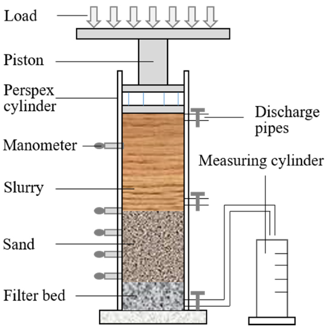
In order to improve the efficiency of the calculations, the dimensions of the numerical models (
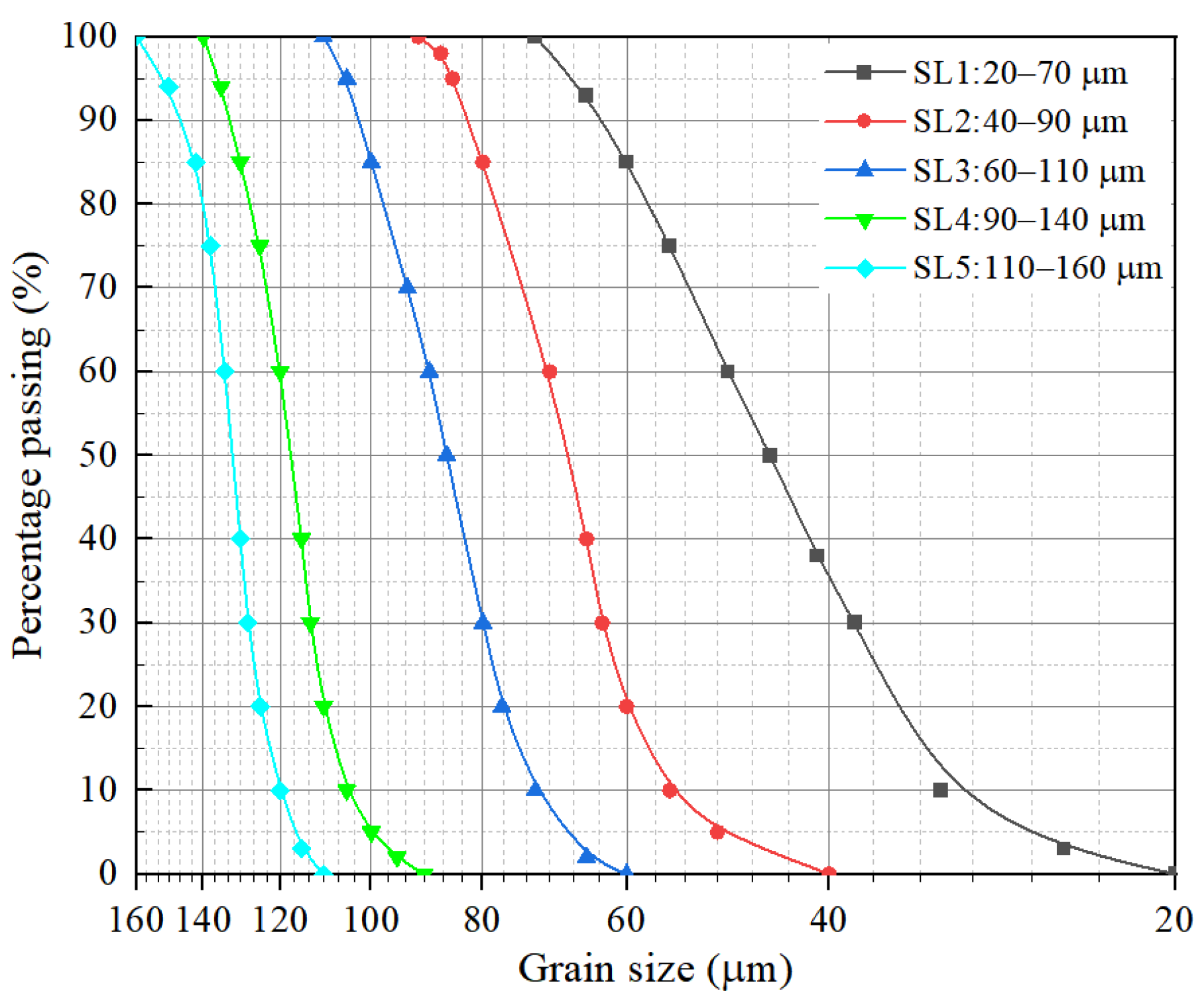
Table 5) in this paper are different from the laboratory test models (Figure 2). However, the difference in the model size does not affect ground porosity and the permeability coefficient trend during the slurry infiltration, but only shortens the infiltration time [34]. Using Darcy’s law, the total duration of the slurry penetration is proportional to the square of the penetration path and inversely proportional to the slurry pressure difference. Because of the large gap between the physical time of the slurry penetration in the numerical calculations and the real slurry penetration time in laboratory tests, the time scale needed to be transformed for a comparative analysis. The test model in Figure 2 was selected as the standard to transform the numerical time, as shown in Table 6.
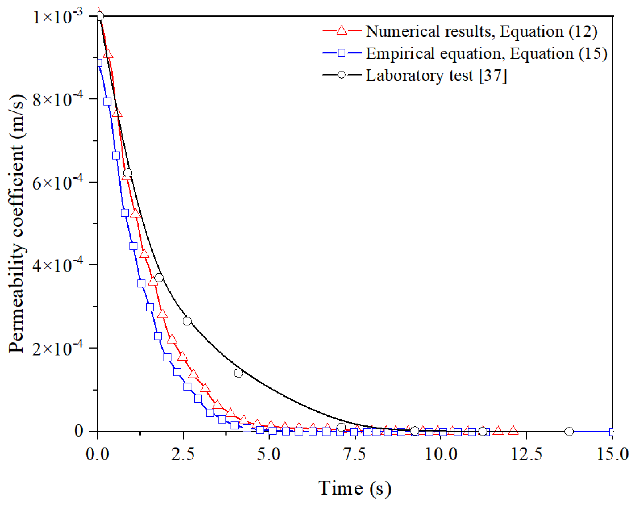
To analyze the permeability coefficient variation during the slurry infiltration, the excess pore water pressure drop on both sides of the infiltration zone and the amount of discharge water in the numerical case ④ (Table 5) were monitored and the permeability coefficient was calculated according to Equation (15). At the same time, the porosity and the average particle size of the infiltration zone in case ④ were monitored, and the permeability coefficient of the sand column was calculated according to Equation (12). The calculation results are shown in Figure 6. Zizka et al. [
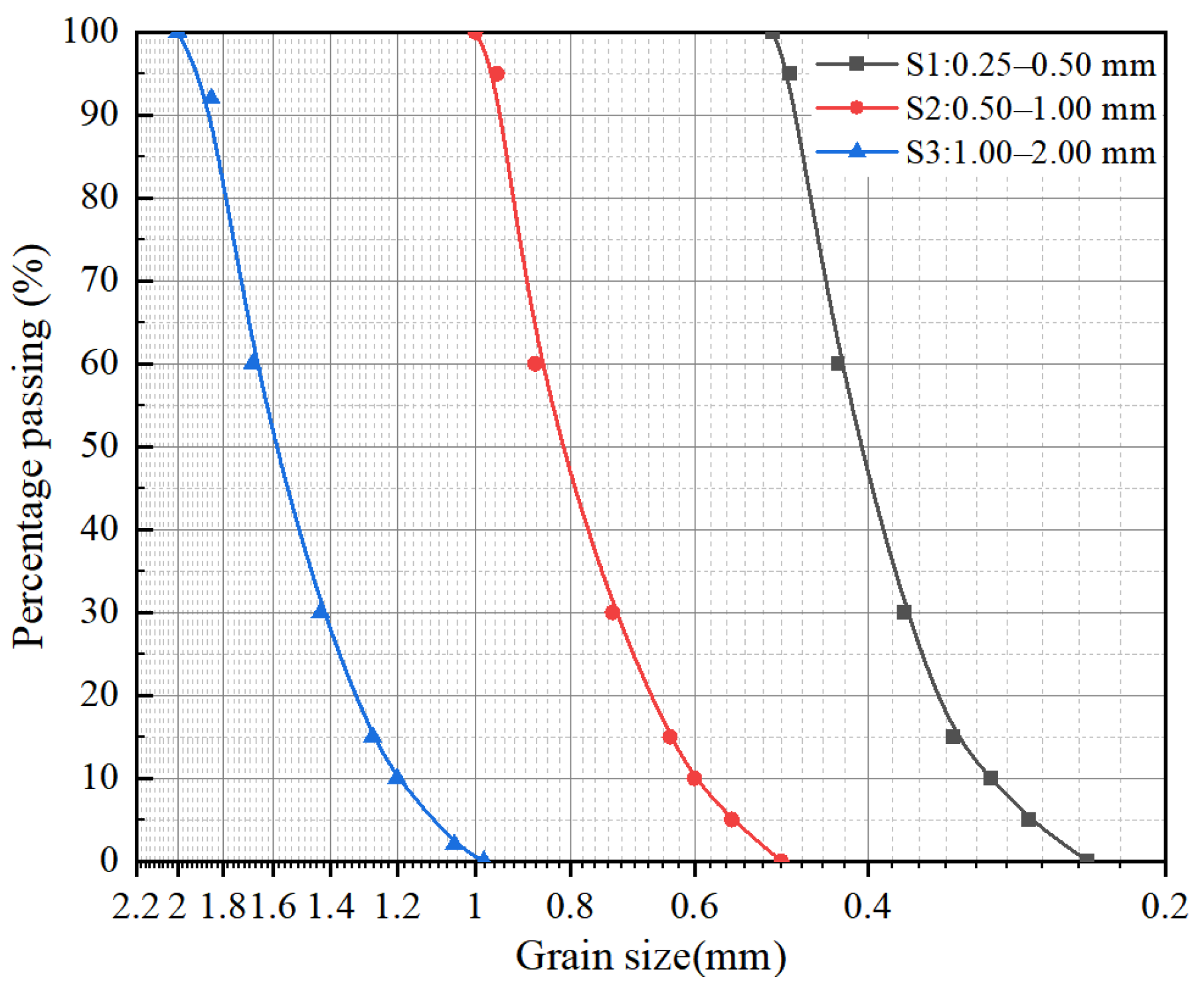
37] monitored the discharge water variation and pore water pressure over time in experiments and calculated the permeability coefficient based on Equation (15). The soil particle size in the third set of tests was in the range between 0.25 and 0.5 mm, and the slurry support pressure was equal to 50 kPa, which was basically consistent with the parameters of numerical case ④. From Figure 6, the results obtained using numerical test data based on Equation (15) were slightly smaller than the permeability coefficients in the numerical simulations. It is probably because the porosity used in Equation (15) is a constant, while the coupling process in the numerical calculations updates the porosity with time. However, in general, the results of the two methods were basically the same, so the numerical model in this paper can reflect the slurry infiltration with accuracy. It should be noted that Zizka et al. [37] used industrial bentonite slurry in their laboratory test, which has a better particle grading, so the slurry penetration process is relatively slow. However, the overall trend of the permeability coefficient is almost the same as in the numerical calculation.

5.2. Type of Slurry Infiltration

The existing laboratory tests [27,37] showed that the penetration pattern of slurry particles in the soil can be divided into three types, type Ⅰ: intact filter cake; type Ⅱ: filter cake + infiltration zone; and type Ⅲ, only infiltration zone. Additionally, the equivalent pore size between the soil particles and the d85 of the slurry particles were used to determine the contact type between the slurry and the soil. The results of the above 12 sets of numerical calculations considering different soils and slurry combinations were analyzed, and the contact types are shown in Table 7. The numerical test results showed that when d85/DP ≥ 1.1, the slurry particles could penetrate the soil pores. An intact filter cake was then formed at the excavation face, as shown in Figure 7b. When 0.6 < d85/DP < 1.1, some slurry particles could enter through the soil pores, and some particles were accumulated at the excavation surface, resulting in a mixed contact form of filter cake + infiltration zone, as shown in Figure 7c. When d85/DP ≤ 0.6, almost all the slurry particles flowed through the soil pores and therefore did not stay at the excavation face, as shown in Figure 7d.
The numerical results showed that both the soil pore size and slurry grade had a significant influence on the slurry permeation behavior. As the ratio d85/D0 decreased, more and more slurry particles entered inside the sand stratum, and fewer particles gathered at the surface, making it less likely to form an intact filter cake. Jia et al. [38] showed that when the slurry density is high enough, even if the ratio d85/D0 is small at the beginning, a filter cake + infiltration zone accumulation pattern can be formed. This is because when the slurry density is high, more slurry particles can fill the soil pores. It will reduce the average pore size of the formation, resulting in an increase in d85/D0. However, it is worth noting that this process will take a long time. Sherard et al. [43] proposed the ratio of D15/d85 to assess the type of slurry/soil contact. When D15/d85 ≤ 5.26, a type 1 filter cake is formed at the excavation surface. When 5.26 < D15/d85 < 10.53, a type 2 contact pattern is formed. When D15/d85 ≥10.53, no slurry particles are trapped at the excavation surface and, therefore, only an infiltration zone is present (type 3). For well-graded soils (Cu ≥ 5 and 1< Cc < 3), the above criteria are usually conservative, as the minimum pore size is smaller. However, when the soil is not particularly well-graded (Cu < 5 or Cc < 1 or Cc ≥3), there is an obvious error for this method. This is because when the soil is poorly graded, the pores in the soil particles are not sufficiently filled by the micro grains. Since the soil particles used in this study are more uniformly graded, the above criteria proposed by Sherard et al. [43] are no longer applicable.

5.3. Slurry Support Mechanism

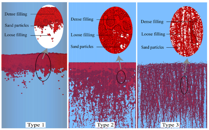
To analyze the formation of the three types of slurry penetration mentioned above from a mechanical point of view, the microscopic distribution patterns of the slurry particles in the soil pores were extracted from the longitudinal profile as shown in Figure 8. For the first type of slurry infiltration, most of the slurry particles are accumulated at the surface of the soil particles, forming a dense and intact filter cake. Only a small fraction of the slurry particles fill the shallow soil pores, while the number of slurry particles entering the soil is minimal and are unable to travel through large distances. They can eventually stagnate in the soil pores forming a loose filling structure. For the second infiltration type, the thickness of the filter cake is significantly reduced, although an intact filter cake can also be formed. Most of the slurry particles are transported to the deeper parts of the soil column. However, the stagnant particles in the shallow part of the soil can form a dense filling network. The sand particles are then tightly packed in the filling network. For the third type of infiltration, slurry particles are almost always transported into the soil pores. Dense filling structures can be formed; the distribution of the filling structures is generally longitudinal.
From the analysis above, during the process of slurry penetration, three main contact mechanisms will occur depending on the ratio of the slurry particle size to the soil pore size. The first type occurs when the slurry particle size is larger than the mean soil pore size (d85 ≥ 1.1 DP) and the slurry particles are stagnantly deposited at the soil surface. As the deposition progresses, a filter cake is then formed at the soil surface. The second type occurs when the slurry particle size is close to the mean soil pore size (0.6 DP < d85 < 1.1 DP); the slurry particles are gradually filled with the pores of the soil particles driven by the hydraulic gradient. With the penetration development, loose filling gradually transforms into dense filling and forms a horizontally distributed dense filling network. Finally, a dense filter cake will form on the sand column surface. The third type occurs when the size of the slurry particles is smaller than the mean pore channel (d85 ≤ 0.6 DP), the slurry particles migrate through the soil pores driven by the hydraulic gradient. The slurry particles will stop moving and will stagnate in the soil pores until the hydraulic gradient is not enough to drive the slurry particles, or they encounter smaller pore channels. The retention of the slurry particles further alters the soil pore structure and affects the slurry penetration. In an engineering project, if bentonite is used as a base material for slurry, the clay particles usually form flocculated clusters [44,45]. As the particle size of the clusters is larger than the soil pore channel’s diameter, they will be stagnantly deposited at the excavation surface. As the deposition progresses, a filter cake will be formed.
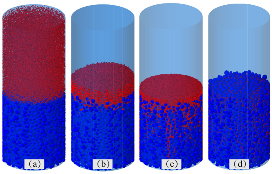
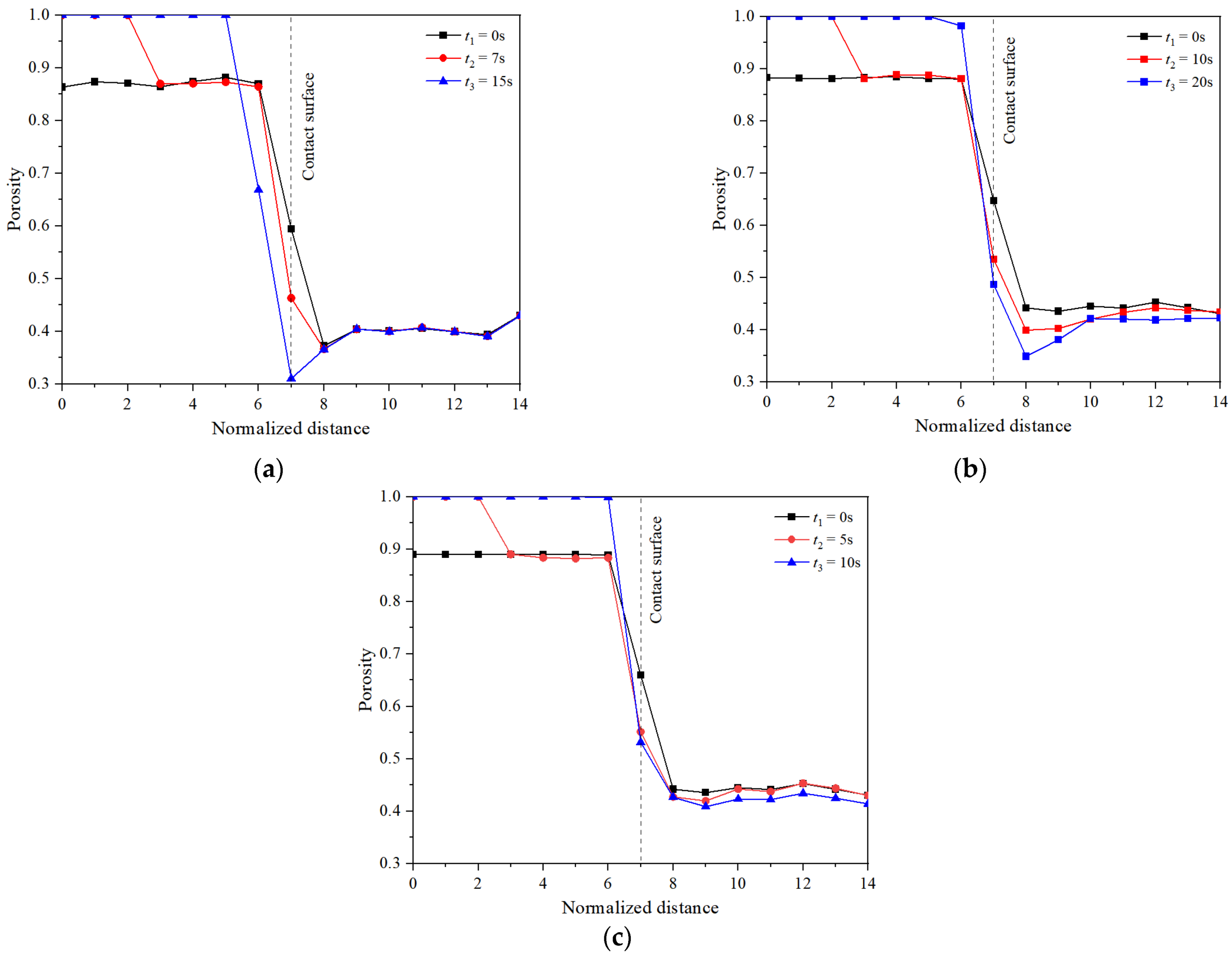
To visually analyze the transport and accumulation of slurry particles during infiltration in the three typical cases, the changes in porosity during calculations are monitored as shown in 
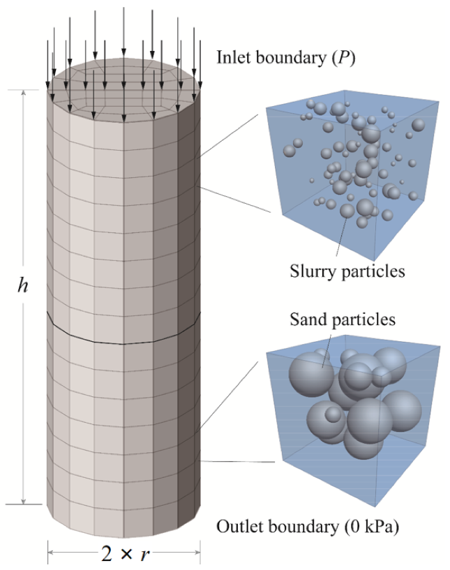
Figure 9. At the beginning of the calculations, the lower half of the model is filled with sand particles and the upper half is filled with slurry (Figure 7a). With the infiltration time ongoing, case ④ showed an obvious decrease in porosity at the slurry–soil contact surface (Figure 9a), while the porosity within the overlying sand column remained essentially unchanged. It indicates that a dense filter cake was formed at the excavation surface. As for case ⑨ (Figure 9b), the decrease in porosity at the slurry–soil contact surface was not so obvious compared with case ④. Because the coarse-grid method was used to calculate the fluid motion, the formation of a thin filter cake over the contact surface did not significantly change the fluid element porosity. The minimum value of porosity occurred below the contact surface because the soil pores at this place were sufficiently filled. In case ⑫ (Figure 9c), the porosity change inside the sand column during the slurry penetration was not so obvious. The porosity at the slurry–soil contact surface remained essentially unchanged, which means that there was no trapped accumulation of slurry particles.

5.4. Analysis of the Slurry Support Effect

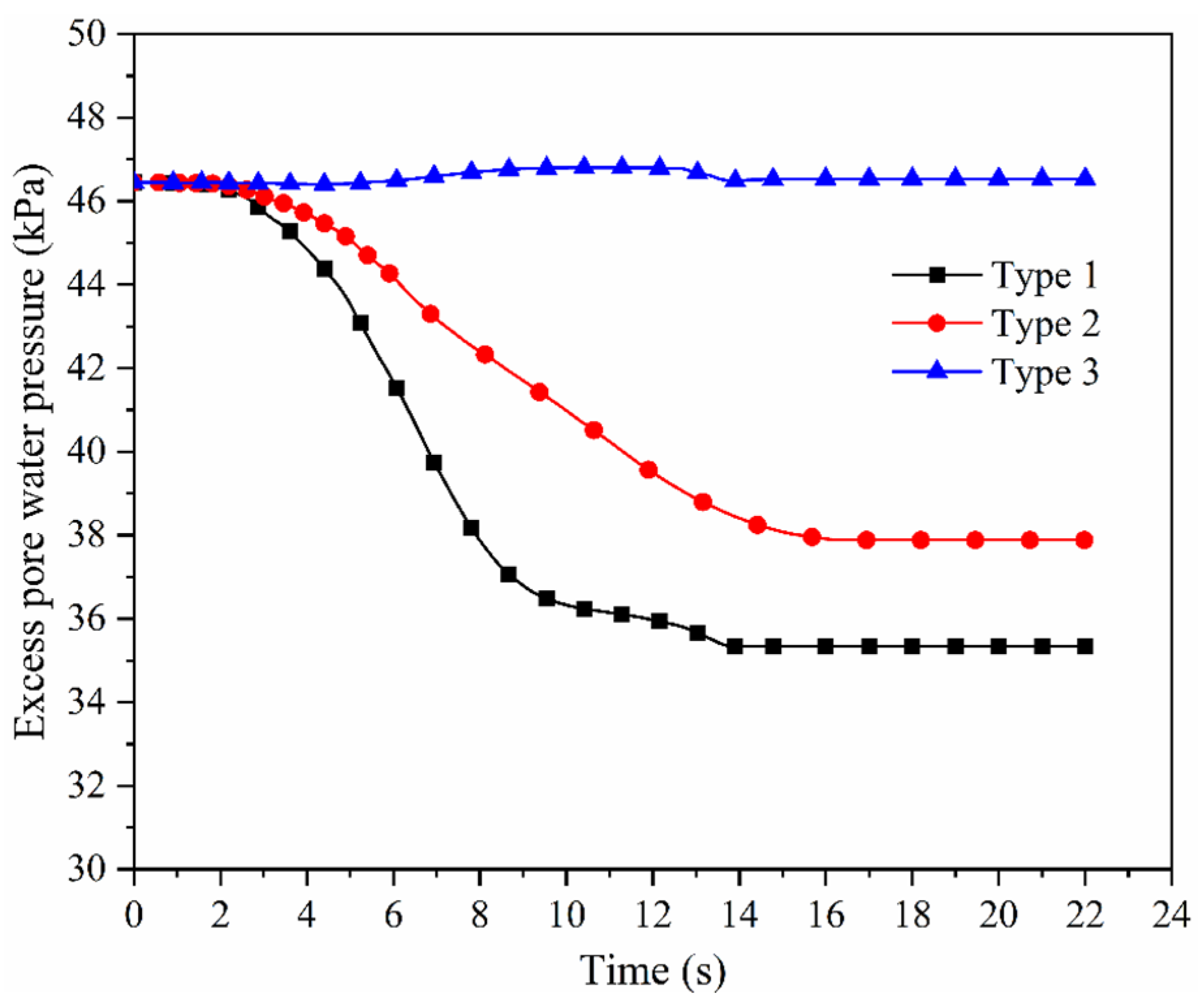
The essence of the slurry support during slurry shield construction is the balancing effect on the soil and water pressure at the tunnel excavation face. Different slurry–soil interaction mechanisms will produce different support effects. The excess pore water pressure overlying the contact layer was monitored during the slurry infiltration as shown in Figure 10. For the first infiltration mechanism (type 1: case ④), the excess pore water pressure in the overlying sand layer under the filter cake decreased significantly and changed at a fast rate. For the second infiltration mechanism (type 2: case ⑨), the excess pore water pressure also decreased but at a slower rate and to a significantly lesser extent than the first mechanism. This was mainly because it takes more time for the slurry particles to fill the soil pores and form a filter cake, which has a smaller thickness. For the third infiltration mechanism (type 3: case ⑫), there was no significant change in excess pore water pressure in the soil layer adjacent to the slurry–soil contact surface. This was because the slurry particles do not form an effective filling network in the soil pores that inhibit the slurry penetration development.
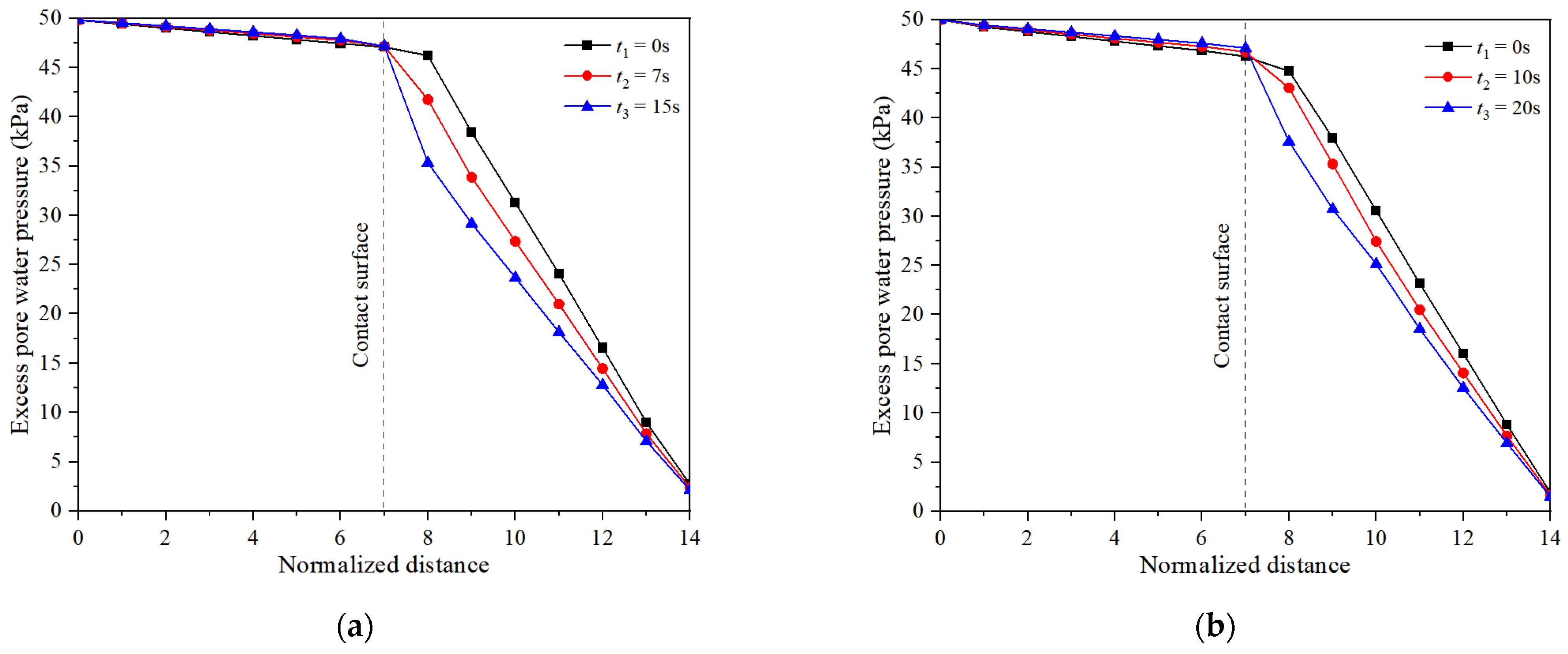
The distribution of excess pore water pressure can effectively reflect the supporting effect of the slurry infiltration. Figure 11 shows the distribution of the excess pore water pressure inside the sand column from three different slurry infiltration types in cases ④, ⑨ and ⑫. As can be seen from Figure 11, there was a small pressure gradient in the slurry itself, but it was negligible. For case ④ in Figure 11a, as the slurry penetration time increased, the excess pore water pressure in the slurry–soil contact layer decreased significantly, about 26% of the entire slurry support pressure. Additionally, the pressure gradient in the slurry–soil contact layer was about 2.4 times the pressure gradient in the sand column. The filter cake formed at the slurry–soil contact surface can lead to a significant reduction in the excess pore water pressure. For case ⑨ in Figure 11b, there was no significant change in the excess pore water pressure in the slurry–soil contact layer at the beginning of the slurry infiltration phase. A slight decrease in the excess pore water pressure was observed within the sand column. As the infiltration time progressed further, there was a decrease in the excess pore water pressure in the slurry–soil contact layer, about 19% of the entire slurry pressure. For case ⑫ in Figure 11c, the excess pore water pressure inside the sand column remained basically unchanged during the whole slurry penetration process. The third type of slurry infiltration mechanism basically cannot achieve the purpose of slurry support.
The filter cake formation can be divided into three different stages by observing the transport of the slurry particles and analyzing the trends in the excess pore water pressure in the soil layer, as well as the soil porosity. In the first stage, soil particles were transported by the slurry particles. The surface soil particles were rearranged during this stage and caused the slurry particles to fill and accumulate in the soil particle pores, forming a permeable zone at the contact surface. This process resulted in a rapid water infiltration into the soil and an instantaneous increase in the excess water pressure in the stratum. In the second stage, the slurry particles continued to accumulate at the contact surface, and the thickness of the filter cake increased. The excess pore water pressure in the overlying layer of the filter cake continued to decrease as the filter cake gradually became denser and denser. In the third stage, the overall permeability coefficient of the denser filter cake became lower and the excess water pressure in the overlying soil body remained stable. It should be noted that the slurry particles are not well-graded in the numerical calculations, so the filter cake formed still has a certain degree of permeability. For the second type of slurry infiltration, both filter cake and slurry infiltration zones are present. Both the dense filling network formed by the slurry particles and the filter cake significantly reduced the excess pore water pressure in the soil body, which means that part of the reduction was successfully converted into an effective support pressure applied to the soil skeleton. For the third type of slurry infiltration, there was no complete dense filling network formed in the direction of the slurry penetration, but only longitudinally extended slurry veins. Therefore, it can hardly change the excess pore water pressure distribution in the soil and cannot effectively ensure the slurry support pressure.

5.5. Time Effect of the Slurry Infiltration

Observations of the three types of slurry–soil interaction reveal that the most obvious difference is the penetration distance of the slurry particles (Figure 8). The transformation effect of the slurry support pressure is closely related to the penetration distance. Larger permeation distance indicates a lower support pressure conversion efficiency [29] as well as a larger slurry particle infiltration loss, which also represents a lower stability coefficient of the tunnel face.
For the support mechanism with both filter cake and infiltration zones, the slurry support effect is mainly shared by the effective support pressure of the filter cake and the shear forces between the slurry particles and the soil pore channel walls. The support pressure generated by the filter cake can be calculated through the excess pore water pressure drop on both sides of it. However, the shear force between the slurry particles and the soil pore channel wall is a microscopic concept and cannot be calculated directly. It is only when the slurry particle transport reaches the maximum penetration distance that the shear force can be in balance with the penetration driving force. Kilchert and Karstedt [43] studied the relationship between the stagnation gradient of the slurry penetration, the characteristic particle size of the soil particles, and the slurry yield strength based on experimental studies [21,46,47]. The formula for the calculation of the maximum penetration distance was modified accordingly:
f so = a τ f , s d 10
l max = Δ S f s o
where fso is the slurry stagnation gradient according to Kilchert and Karstedt [16] (kPa/m). a is the empirical factor from the experiments; the value can be 2 or 3.5. d10 is the characteristic grain size of soil (10% passage in sieve analysis, mm). τf,s is the static yield point of the slurry (Pa). △S is the slurry excess pressure (kPa). lmax is the maximum slurry penetration depth (m).
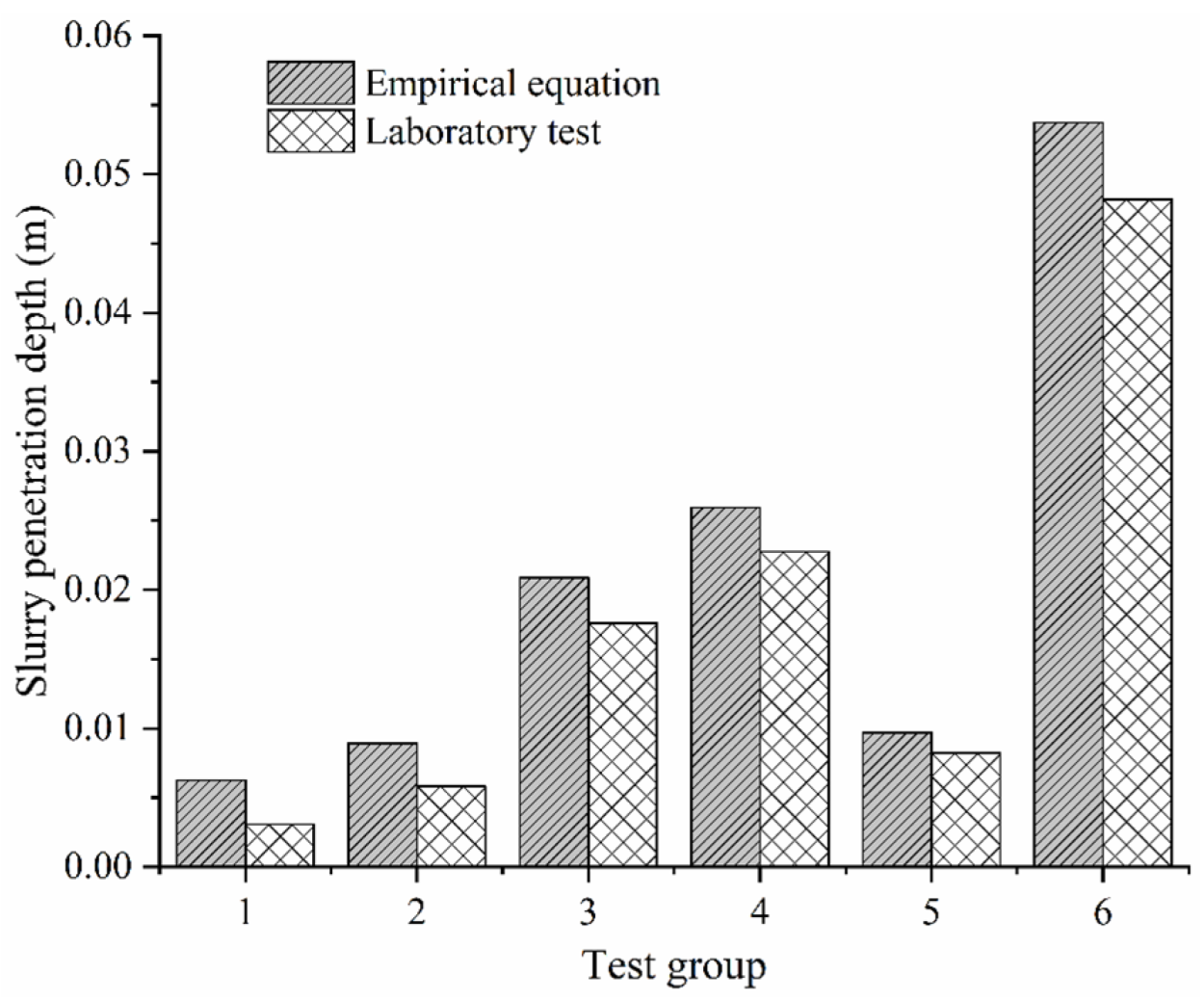
Zizka et al. [37] carried out a series of experiments to study the patterns of the slurry infiltration and calculated the slurry infiltration distance by real-time drainage monitoring. A comparison of the slurry permeation distances in the experiments and the empirical formula calculations are shown in Figure 12. The empirical formula calculates a larger permeation distance compared to the experimental monitoring. This is because the slurry will change the soil grading during the penetration process, which will reduce the characteristic grain size (d10) of the soil body. Therefore, a larger slurry stagnation gradient is obtained, which will eventually lead to the reduction in the slurry permeation distance according to Equation (16).
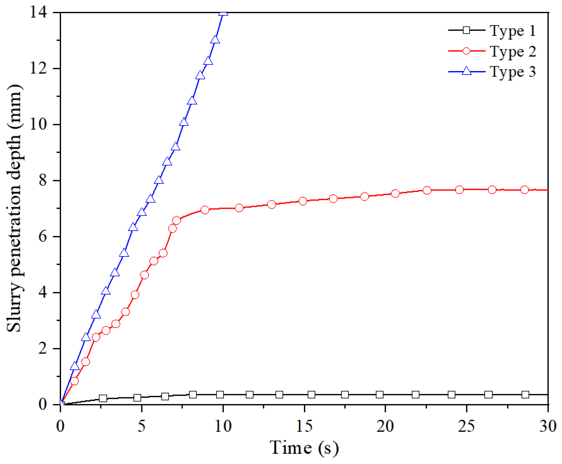
The maximum penetration distance is determined by the final state of the slurry penetration and does not consider the time effect. Once the slurry penetrates over long distances in a short period and produces large slurry losses, it may lead to a destabilization of the tunnel face. Therefore, the development process of the slurry penetration distance has a significant influence on the slurry support effectiveness. The displacement of the slurry particles is monitored in the numerical calculations as shown in Figure 13. It can be seen from the figure that for the first type of interaction mechanism, the slurry particles are not transported in the soil, but almost completely stagnate and accumulate at the soil surface. For the second type of slurry penetration mechanism, the slurry particles move faster at the beginning of the penetration, but with the gradual formation of the dense filling network, the penetration distance gradually stabilizes. For the third type of slurry penetration mechanism, the penetration distance of the slurry particles increases linearly during penetration, and when the sand column is not high enough, slurry particles tend to penetrate the entire sand column.
Anagnostou and Kovári [29] proposed a time-dependent formula for the theoretical calculation of the slurry penetration distance based on the assumption of a one-dimensional infiltration at the tunnel face. The slurry penetration distance is determined by the soil permeability coefficient and the viscosity ratio of the slurry to water.
t = n μ s γ w Δ S k w μ w f so 2 [ l l max ln ( 1 l l max ) ]
where t is the timespan since the slurry penetration start (s). n is the soil porosity. μs is the slurry dynamic viscosity (Pa·s). γw is the water unit weight (kN/m3). △S is the slurry excess pressure (kPa). l is the penetration distance at the timespan t (m). lmax is the maximum penetration distance of the slurry (m). kw is the permeability coefficient of soil for water (m/s). μw is the dynamic viscosity of water (Pa·s). fso is the slurry stagnation gradient (kPa/m).
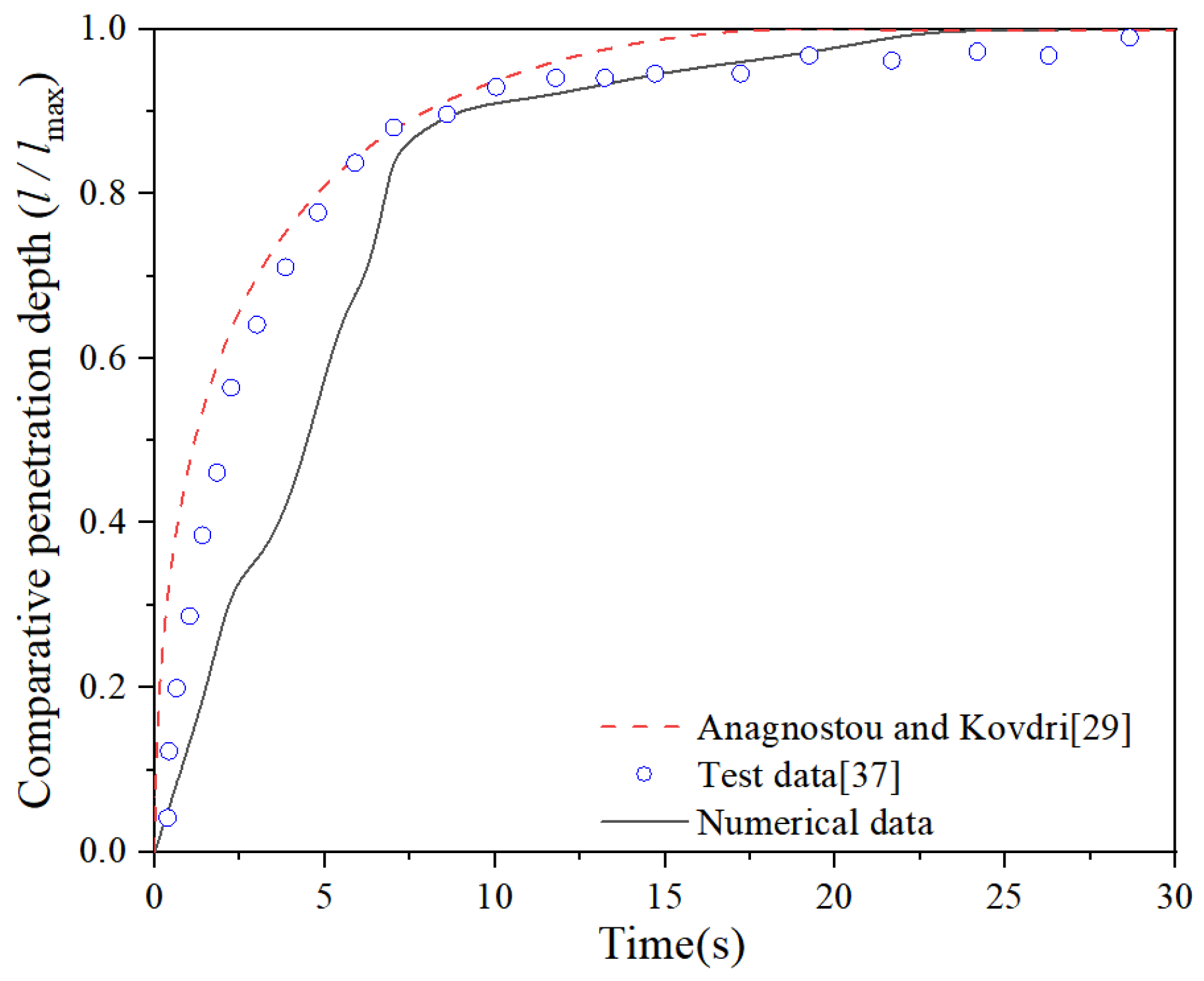
The slurry penetration distance is compared as a dimensionless number with the empirical formula [29] based on the slurry penetration development in numerical case ⑨. At the same time, the data of the slurry infiltration with similar combinations (soil particle size range: 0.5–1.0 mm, porosity: 0.41, slurry density: 1.03 g/cm3, and slurry concentration of 5.5%) in the laboratory tests [37] are shown in Figure 14. The development of the penetration distance obtained by the three methods is almost identical. However, the empirical formula as well as the laboratory tests have a faster penetration rate, especially the empirical formula, which shows a significantly larger penetration rate at the beginning of the test. Although, the empirical formula uses constant calculation parameters such as the stagnation gradient and porosity, but once the maximum permeation distance can be determined, the empirical formula reflects the development of the slurry permeation distance. It is in good agreement with the numerical and test results. The exponential relationship of the empirical formula can well reflect the influence of the slurry penetration process on the permeation rate due to the stagnant accumulation of particles.
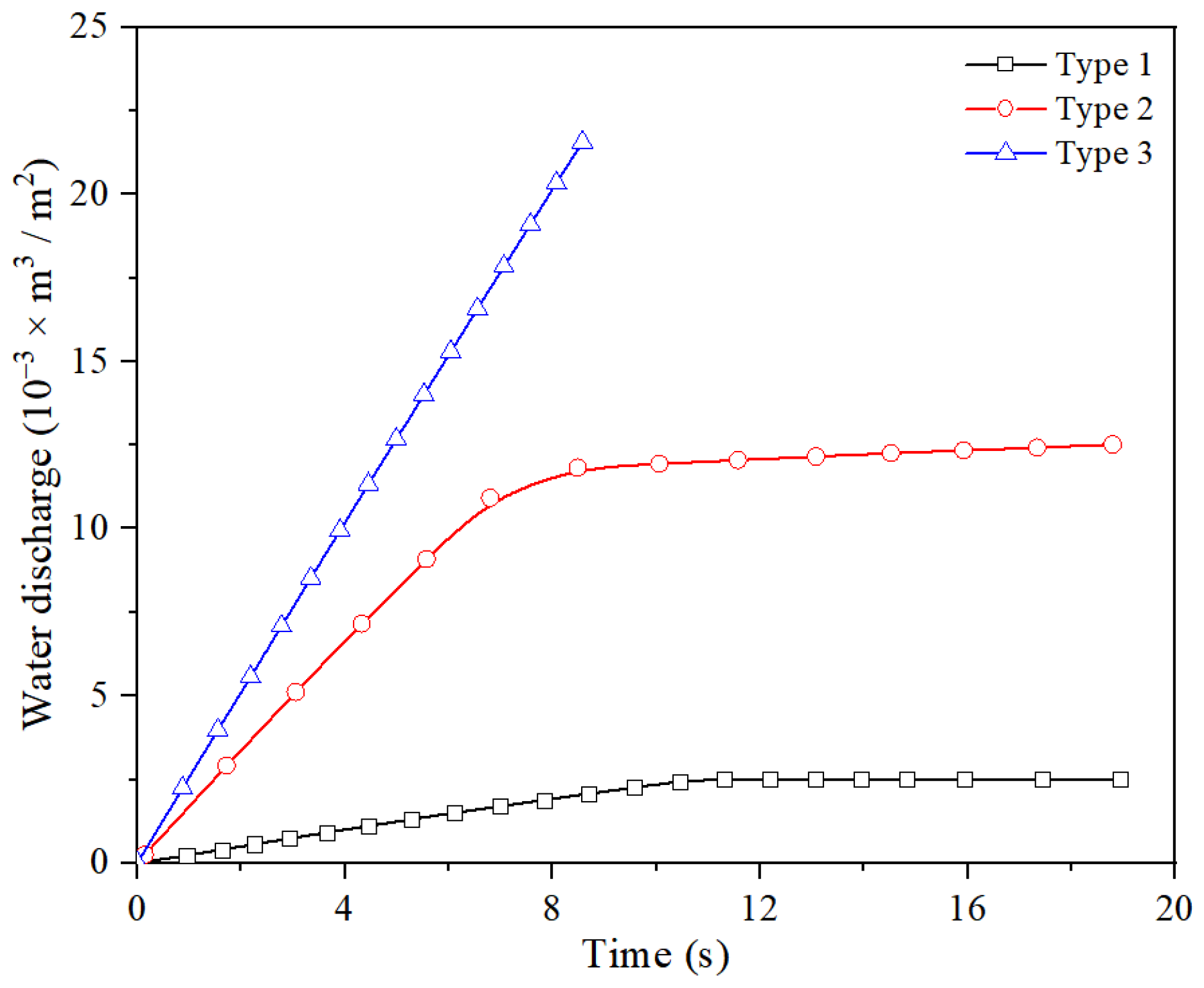
During shield tunneling, the filter cake formed at the tunnel face is a dynamic process, this is because the filter cake is always in a cycle of the following type: formed, destroyed and re-formed. Therefore, it is required that the filter cake is formed quickly, which means that the slurry particles fill the soil pores quickly with a small amount of slurry filtration loss. A dense filter cake will then be formed at the tunnel face, sealing the excavation surface to maintain the stability of the tunnel face. The filter cake formation time, as well as the amount of slurry filtration loss during the formation process and the excess pore water pressure in the ground after the formation are often used as important indicators for evaluating the filter cake quality and the effect of the slurry support. However, real-time observation of the filter cake quality and monitoring of the excess pore water pressures are not feasible during a real tunnel excavation. The slurry filtration loss and the water discharge during infiltration can be monitored. These indicators can be obtained by calculating the amount of slurry injection and slag discharge, and therefore can be used as key indicators to evaluate the filter cake quality. Water discharge for the three different slurry infiltration mechanisms were monitored during numerical calculations and are shown in Figure 15.
For the first slurry infiltration type, the discharge water grew very slowly. It is because the slurry particle size distribution was not well graded; the filter cake formed was still permeable to a certain extent. The cumulative discharge water was around 4 × 10⁻³ m3/m2 for a slurry excess pressure of 50 kPa. For the second type of slurry infiltration, the water discharge increased more rapidly at the beginning of the infiltration, but after about 7 s, the discharge volume tended towards a stable value of 12 × 10−3 m3/m2. For the third infiltration type, the drainage trend at the beginning of the slurry infiltration was like the second type. However, with the infiltration development, the drainage volume quickly overtook the second infiltration type and did not reach a steady value. An analysis of the discharge water corresponding to the three types of slurry infiltration indicated that the formation of an intact filter cake could effectively inhibit the drainage increase, and the slurry support effect could be achieved in a short period. The purely infiltration mechanism could not effectively control the drainage development and could not achieve the slurry support effect, accompanied by the presence of a high excess pore water pressure in the stratum. For the second type of slurry penetration, as the slurry particles filled and stacked inside the soil pores, the pore structure of the soil changed and an intact filter cake could eventually be formed. However, the whole process was slower compared to the first type of slurry infiltration.

6. Conclusions

In this paper, coupled CFD-DEM numerical models are used to simulate the slurry penetration in a sand column under different soil-grading combinations. The slurry infiltration phenomenon and the corresponding pressure transfer mechanisms are shown through a numerical parametric study. The slurry support effect produced by different slurry infiltration types is analyzed. The following findings can be drawn from the current study:
(1)
There are three types of infiltration interactions between slurry and sand particles. When the slurry particle size is larger than the mean soil pore size (d85 ≥ 1.1 DP), the slurry particles are stagnantly deposited at the soil surface, and finally an intact filter cake will be formed. When the slurry particle size is close to the mean soil pore size (0.6 DP < d85 < 1.1 DP), the slurry particles will gradually fill the soil pores driven by the hydraulic gradient. With the development of penetration, loose filling will gradually transform into a dense filling network, and finally an intact filter cake will be formed. When the size of the slurry particles is smaller than the mean soil pore size (d85 ≤ 0.6 DP), the slurry particles will migrate through the soil pores.
(2)
The dense filling of soil pores by slurry particles significantly increases the water pressure gradient in the infiltration zone, which leads to a decrease in the pressure gradient within the deep soil. The slurry particles in the surface layer become denser and denser driven by the larger pressure gradient, and eventually develop into a dense filter cake. Once an intact filter cake or dense filling network is formed, a large excess pore water pressure drop will occur on both sides of the filter cake. The reduced excess pore water pressure on the inner side is the effective slurry support pressure acting on the soil skeleton. In that way, the slurry support pressure can eventually be converted to an effective support pressure.
(3)
The slurry infiltration process has an obvious time effect, in which the penetration distance of slurry particles entering the interior of the soil pore space gradually increases with time. The slurry penetration distance is an important evaluation index of the slurry support pressure efficiency. The larger the penetration distance, the worse the support pressure efficiency. The penetration distance varies nonlinearly with time and eventually tends to a constant value. However, for the purely infiltration zone mechanism, the slurry penetration distance basically changes linearly within the sand column height, which will result in large slurry filtration loss eventually.

Author Contributions

Conceptualization, K.L. and W.D.; methodology, K.L.; software, W.D.; validation, K.L., W.D. and C.Q.; formal analysis, W.D.; investigation, W.D.; resources, K.L.; data curation, W.D.; writing—original draft preparation, K.L.; writing—review and editing, W.D.; visualization, C.Q.; supervision, W.D.; project administration, W.D. All authors have read and agreed to the published version of the manuscript.

Funding

This research was funded by the Fundamental Research Funds for the Central Universities (Grant No. N2201017) and the Natural Science Foundation of Shandong Province (Grant No. ZR2021ME135).

Institutional Review Board Statement

Not applicable.

Informed Consent Statement

Not applicable.

Data Availability Statement

The data provided in this study could be released upon reasonable request.

Conflicts of Interest

The authors declare no conflict of interest.

References

  1. Horn, M. Horizontal earth pressure on perpendicular tunnel face. In Hungarian National Conference of the Foundation Engineer Industry; Hungary Press: Budapest, Hungary, 1961; pp. 7–16. [Google Scholar]
  2. Anagnostou, S.T.G. The contribution of horizontal arching to tunnel face stability. Geotechnik 2012, 35, 34–44. [Google Scholar] [CrossRef]
  3. Anagnostou, G.; Perazzelli, P. The stability of a tunnel face with a free span and a non-uniform support. Geotechnik 2013, 36, 40–50. [Google Scholar] [CrossRef]
  4. Leca, E.; Dormieux, L. Upper and lower bound solutions for the face stability of shallow circular tunnels in frictional material. Géotechnique 1990, 40, 581–606. [Google Scholar] [CrossRef] [Green Version]
  5. Soubra, A.H. Kinematical approach to the face stability analysis of shallow circular tunnels. In Proceedings of the 8th International Symposium on Plasticity, Vancouver, BC, Canada, 2000; pp. 443–445. Available online: https://hal.archives-ouvertes.fr/hal-01008370 (accessed on 14 September 2022).
  6. Subrin, D.; Wong, H. Stabilité du front d’un tunnel en milieu frottant: Un nouveau mécanisme de rupture 3D. CR Mécanique. 2002, 330, 513–519. [Google Scholar] [CrossRef]
  7. Ding, W.; Liu, K.; Shi, P.; Li, M.; Hou, M. Face stability analysis of shallow circular tunnels driven by a pressurized shield in purely cohesive soils under undrained conditions. Comput. Geotech. 2018, 107, 110–127. [Google Scholar] [CrossRef]
  8. Mollon, G.; Dias, D.; Soubra, A.-H. Face Stability Analysis of Circular Tunnels Driven by a Pressurized Shield. J. Geotech. Geoenviron. 2010, 136, 215–229. [Google Scholar] [CrossRef] [Green Version]
  9. Mollon, G.; Dias, D.; Soubra, A.-H. Rotational failure mechanisms for the face stability analysis of tunnels driven by a pressurized shield. Int. J. Numer. Anal. Methods Géoméch. 2010, 35, 1363–1388. [Google Scholar] [CrossRef] [Green Version]
  10. Huang, M.; Li, S.; Yu, J.; Tan, J.Q.W. Continuous field based upper bound analysis for three-dimensional tunnel face stability in undrained clay. Comput. Geotech. 2018, 94, 207–213. [Google Scholar] [CrossRef]
  11. Zou, J.; Chen, G.; Qian, Z. Tunnel face stability in cohesion-frictional soils considering the soil arching effect by improved failure models. Comput. Geotech. 2018, 106, 1–17. [Google Scholar] [CrossRef]
  12. Zhang, C.; Li, W.; Zhu, W.; Tan, Z. Face stability analysis of a shallow horseshoe-shaped shield tunnel in clay with a linearly increasing shear strength with depth. Tunn. Undergr. Space Technol. 2020, 97, 103291. [Google Scholar] [CrossRef]
  13. Zhang, Y.; Gong, G.; Yang, H.; Li, W.; Liu, J. Precision versus intelligence: Autonomous supporting pressure balance control for slurry shield tunnel boring machines. Autom. Constr. 2020, 114, 103173. [Google Scholar] [CrossRef]
  14. Morgenstern, N.; Amir-Tahmasseb, I. The Stability of a Slurry Trench in Cohesionless Soils. Géotechnique 1965, 15, 387–395. [Google Scholar] [CrossRef]
  15. Müller-Kirchenbauer, H. Stability of slurry trenches. In Proceedings of the 5th European Conference on Soil Mechanics and Foundation Engineering, Madrid, Spain, 10–13 April 1972; pp. 543–553. [Google Scholar]
  16. Kilchert, M.; Karstedt, J. Band 2 Standsicherheitsberechnung von Schlitzwaenden nach DIN 4126; Bauverlag GmbH (Beuth-Kommentare): Wiesbaden/Berlin, Germany, 1984. [Google Scholar]
  17. Zizka, Z.; Schoesser, B.; Thewes, M. Investigations on transient support pressure transfer at the tunnel face during slurry shield drive part 1: Case A–Tool cutting depth exceeds shallow slurry penetration depth. Tunn. Undergr. Space Technol. 2021, 118, 104168. [Google Scholar] [CrossRef]
  18. Talmon, A.M.; Mastbergen, D.R.; Huisman, M. Invasion of Pressurized Clay Ssuspension into Granular Soil. J. Porous Media 2013, 351–365. [Google Scholar] [CrossRef]
  19. Watanabe, T.; Yamazaki, H. Giant size slurry shield is a success in Tokyo. Tunn. Tunnell. 1981, 13, 13–17. [Google Scholar]
  20. Khan, R.A.; Sharma, R. Strength and Durability Characteristics of Rice Husk Ash Concrete Reinforced with Polypro-pylene Fibres. Jordan J. Civ. Eng. 2018, 12, 653–668. [Google Scholar]
  21. Simons, H.; Ruppert, F. Entwicklung geeigneter Verfahren zum Messen der physikalischen Eigenschaften von Ben-tonitsuspensionen auf Baustellen. In Mitteilung des Lehrstuhls für Grundbau und Bodenmechanik; Technische Universität: Braunschweig, Germany, 1982. [Google Scholar]
  22. Cheng, Z.L.; Wu, Z.M.; Xu, Y.Y. Experimental study on stability of excavation face of slurry shield tunnel construction in sandy ground. J. Yangtze River Sci. Res. Institute. 2001, 18, 53–55. (In Chinese) [Google Scholar]
  23. Fritz, P. Additives for Slurry Shields in Highly Permeable Ground. Rock Mech. Rock Eng. 2006, 40, 81–95. [Google Scholar] [CrossRef]
  24. Fritz, P.; Hermanns, S.R.; Heinz, A. Modified bentonite slurries for slurry shields in highly permeable soils. In Proceedings of the 4th International Symposium Geotechnical Aspects of Underground Construction in Soft Ground, Toulouse, France, 28–31 August 2002. [Google Scholar]
  25. Han, X.R.; Zhu, W.; Liu, Q.W.; Zhong, X.C.; Min, F.L. Influence of slurry property on filter cake quality on working face of slurry shield. Rock Soil Mech. 2008, 29, 288–292. (In Chinese) [Google Scholar]
  26. Min, F.-L.; Zhu, W.; Han, X.-R.; Zhong, X.-C. The Effect of Clay Content on Filter-Cake Formation in Highly Permeable Gravel. Geotech. Spec. Publ. 2010, 204, 210–215. [Google Scholar] [CrossRef]
  27. Min, F.; Zhu, W.; Han, X. Filter cake formation for slurry shield tunneling in highly permeable sand. Tunn. Undergr. Space Technol. 2013, 38, 423–430. [Google Scholar] [CrossRef]
  28. Krause, T. Schildvortrieb Flüssigkeitsgestuetzte Ortsbrust. Master’s Thesis, Technische Universität, Braunschweig, Germany, 1987. [Google Scholar]
  29. Anagnostou, G.; Kovdri, K. The face stability of slurry-shield-driven tunnels. Tunn. Undergr. Sp. Tech. 1994, 9, 165–174. [Google Scholar] [CrossRef]
  30. Xu, T.; Bezuijen, A. Analytical methods in predicting excess pore water pressure in front of slurry shield in saturated sandy ground. Tunn. Undergr. Space Technol. 2018, 73, 203–211. [Google Scholar] [CrossRef]
  31. Zhang, Z.; Yin, T.; Huang, X.; Dias, D. Slurry filtration process and filter cake formation during shield tunnelling: Insight from coupled CFD-DEM simulations of slurry filtration column test. Tunn. Undergr. Space Technol. 2019, 87, 64–77. [Google Scholar] [CrossRef]
  32. Itasca Consulting Group Inc. PFC 5.0 Documentation. Available online: https://www.itascacg.com/software/pfc (accessed on 20 October 2019).
  33. Tsuji, Y.; Kawaguchi, T.; Tanaka, T. Discrete particle simulation of two-dimensional fluidized bed. Powder Technol. 1993, 77, 79–87. [Google Scholar] [CrossRef]
  34. Wang, Y.; Chai, J.; Xu, Z.; Qin, Y.; Wang, X. Numerical Simulation of the Fluid–Solid Coupling Mechanism of Internal Erosion in Granular Soil. Water 2020, 12, 137. [Google Scholar] [CrossRef] [Green Version]
  35. Guyer, J.E.; Wheeler, D.; Warren, J.A. FiPy: Partial Differential Equations with Python. Comput. Sci. Eng. 2009, 11, 6–15. [Google Scholar] [CrossRef]
  36. Eichholz, C.; Nirschl, H.; Chen, F.; Hatton, T.A. DEM-simulation of the magnetic field enhanced cake filtration. AIChE J. 2012, 58, 3633–3644. [Google Scholar] [CrossRef]
  37. Zizka, Z.; Schoesser, B.; Thewes, M.; Schanz, T. Slurry Shield Tunneling: New Methodology for Simplified Prediction of Increased Pore Pressures Resulting from Slurry Infiltration at the Tunnel Face Under Cyclic Excavation Processes. Int. J. Civ. Eng. 2018, 17, 113–130. [Google Scholar] [CrossRef]
  38. Rui, J.; Wei, Z.; Fan-Lu, M. Effect of Particle Size Distribution of Slurry and Pore Size of Stratum on Formation of Filter Cake in Slurry Shield. China J. Highw. Transp. 2017, 30, 100–108. [Google Scholar] [CrossRef]
  39. Yang, D.; Xia, Y.M.; Wu, D.; Chen, P.; Zeng, G.Y.; Zhao, X.Q. Numerical investigation of pipeline transport character-istics of slurry shield under gravel stratum. Tunn. Undergr. Space Technol. 2018, 71, 223–230. [Google Scholar] [CrossRef]
  40. Bonkinpillewar, P.D.; Kulkarni, A.; Panchagnula, M.V.; Vedantam, S. A novel coupled fluid–particle DEM for simulating dense granular slurry dynamics. Granul. Matter 2015, 17, 511–521. [Google Scholar] [CrossRef]
  41. Wei, X.; Min, F.L.; Zhong, X.C. Slurry and Filter Cake in Slurry Shield; Science Press: Beijing, China, 2016. [Google Scholar]
  42. Kawano, K. Numerical Evaluation of Internal Erosion Due to Seepage Flow. Ph.D. Thesis, Imperial College London, London, UK, 2016. [Google Scholar]
  43. Sherard, J.L.; Dunnigan, L.P.; Talbot, J.R. Basic Properties of Sand and Gravel Filters. J. Geotech. Eng. 1984, 110, 684–700. [Google Scholar] [CrossRef]
  44. Mehta, A.J.; Lee, S.C. Problems in linking the threshold condition for thetransport of cohesionless and cohesive sediment grain. J. Coastal Res. 1993, 10, 170–177. [Google Scholar]
  45. Pierre, A.C.; Ma, K.; Barker, C. Structure of kaolinite floes formed in an aqueous medium. J. Mater. Sci. 1995, 30, 2176–2181. [Google Scholar] [CrossRef]
  46. Weiss, F. Die Standfestigkeit Flüssigkeitsgestützter Erdwände; Ernst & Sohn: München, Germany, 1967. [Google Scholar]
  47. Müller-Kirchenbauer, H. Zur Standsicherheit von Schlitzwänden in geschichteten Baugrund; Veröffentlichung des Grundbauinstitus der Technicschen Universität Berlin: Berlin, Germany, 1977; Volume 1, pp. 72–88. [Google Scholar]
Figure 1. Coupling mode and information exchange process of the two components.
Buildings 12 01744 g001
Figure 2. Schematic diagram of an infiltration column test.
Buildings 12 01744 g002
Figure 3. Schematic diagram of fluid elements with particles inside.
Buildings 12 01744 g003
Figure 4. Particle grain size distribution curves for three kinds of sand.
Buildings 12 01744 g004
Figure 5. Particle grain size distribution curves for five kinds of slurry.
Buildings 12 01744 g005
Figure 6. Permeability coefficient development with time.
Buildings 12 01744 g006
Figure 7. Slurry infiltration type (a) initial infiltration model; (b) type 2: intact filter cake (case ④); (c) type 2: filter cake + infiltration zone (case ⑨); (d) type 3: purely infiltration zone (case ⑫).
Buildings 12 01744 g007
Figure 8. Mechanisms of slurry–soil interaction.
Buildings 12 01744 g008
Figure 9. Soil porosity distribution. (a) case ④; (b) case ⑨; (c) case ⑫. (The normalized distance represents the ratio of the distance from the pressure loading to the longitudinal fluid elements scale.)
Buildings 12 01744 g009
Figure 10. Changes in excess pore water pressure under the slurry–soil contact surface.
Buildings 12 01744 g010
Figure 11. Longitudinal excess pore water pressure distribution: (a) case ④; (b) case ⑨; (c) case ⑫.
Buildings 12 01744 g011aBuildings 12 01744 g011b
Figure 12. Comparison of the slurry penetration distance [37].
Buildings 12 01744 g012
Figure 13. Development of slurry penetration distance.
Buildings 12 01744 g013
Figure 14. Time dependent slurry penetration depth.
Buildings 12 01744 g014
Figure 15. Water discharge for three different slurry infiltration mechanisms.
Buildings 12 01744 g015
Table 1. Soil particle parameters.
ParametersValue
Volumetric weight2000 kg/m3
Young’s modulus70 GPa
Poisson’s ratio0.3
Friction coefficient0.5
Restitution0.3
Particle number5689~5877
Diameter250~2000 μm
Contact modelHertz
Table 2. Slurry parameters.
ItemsParametersValue
Slurry particleVolumetric weight2000 kg/m3
Young’s modulus5 MPa
Poisson’s ratio0.3
Friction coefficient0.05
Restitution0.3
Particle number28,461~371,083
Diameter20~160 μm
Contact modelHertz
FluidVolumic weight1000 kg/m3
Kinematic viscosity1 × 10−6 m2/s
Fluid typeNewtonian
Table 3. Physical parameters of the soil.
Soil TypesParticle Size, D/(μm)Coefficient of Nonuniformity, CuCoefficient of Curvature,CcMean Grain Size, D0/(μm)Permeability Coefficient k/(m·s−1)Average Pore Size, DP/(μm)
S1250~5001.431.053750.00171
S2500~10001.451.017500.004142
S31000~20001.401.0215000.016285
Table 4. Slurry particle parameters.
Slurry TypesSlurry Particle Size d/(μm)Characteristic Grain Size, d85/(μm)Coefficient of Nonuniformity, CuCoefficient of Curvature, Cc
SL120~70601.530.92
SL240~90801.271.03
SL360~1101001.241.00
SL490~1401301.141.01
SL5110~1601421.121.02
Table 5. Parametric study.
Case NumbersParticle Size, D/(μm)Average Pore Size, DP/(μm)Characteristic Grain Size, d85/(μm)d85/DPModel Size,(*r × h: mm)Particles Number, (Soil/Slurry)
S1:250~50071SL1:600.83 × 155826/185,525
SL2:801.15826/126,488
SL3:1001.45826/94,254
SL4:1301.85826/42,850
SL5:1422.05826/28,461
S2:500~1000142SL1:600.46 × 305689/371,083
SL2:800.65689/329,737
SL3:1000.75689/226,017
SL4:1300.95689/121,898
SL5:1421.05689/113,724
S3:1000~2000285SL3:1000.412 × 605877/287,564
SL5:1420.55877/206,351
*r represents the radius of the numerical model and h represents the height of the numerical model (Figure 3).
Table 6. Standardized slurry penetration time conversions.
ItemsPenetration Path, L(mm)Slurry Pressure Difference, △P(kPa)Permeability Coefficient, k(mm/s)Permeability Time, t(s)
Test modelL = 200P = 50k1t
Numerical modela × Lb × △Pk2 t c · ( k 2 · b k 1 · a 2 )
Note: tc represents the physical time of the slurry infiltration for the numerical calculations; a and b represent the calculation factors of penetration path and pressure difference, respectively.
Table 7. Relationship between the slurry–soil contact type and combination sets.
Soil
Slurry
S1S2S3
d85/DP*D15/d85Typed85/DPD15/d85Typed85/DPD15/d85Type
SL10.85.520.410.63---
SL21.14.110.67.93---
SL31.43.310.76.420.412.73
SL41.82.510.94.92---
SL52.02.311.04.520.58.93
*D15 represents the size of a sand particle that is larger than 15% of the total particles.
Publisher’s Note: MDPI stays neutral with regard to jurisdictional claims in published maps and institutional affiliations.

