Data Reconstruction of Wireless Sensor Network and Zonal Demand Control in a Large-Scale Indoor Space Considering Thermal Coupling

Abstract

An indoor high and open space is characterized by high mobility of people and uneven temperature distribution, so the conventional design and operation of air conditioning systems makes it difficult to regulate the air conditioning system precisely and efficiently. Thus, a Wireless Sensor Network was constructed in an indoor space located in Hong Kong to monitor the indoor environmental parameters of the space and improve the temperature control effectively. To ensure the continuity of the measurement data, three algorithms for reconstructing temperature, relative humidity and carbon dioxide data were implemented and compared. The results demonstrate the accuracy of support vector regression model and multiple linear regression model is higher than Back Propagation neural network model for reconstructing temperature data. Multiple linear regression is the most convenient from the perspective of program complexity, computing speed and difficulty in obtaining input conditions. Based on the data we collected, the traditional single-input-single-output control, zonal temperature control and the proposed zonal demand control methods were modeled on a Transient System Simulation Program (TRNSYS) control platform, the thermal coupling between the subzones without physical partition was taken into account, and the mass transfer between the virtual boundaries was calculated by an external CONTAM program. The simulation results showed the proposed zonal demand control can alleviate the over-cooling or over-heating phenomenon in conventional temperature control, thermal comfort and energy reduction is enhanced as well.

1. Introduction

A large-scale indoor space is characterized by a high height and a large indoor area. From the perspective of indoor temperature control, the most typical features of that space is the uneven internal temperature distribution. The conventional air conditioning with uniform supply and cooling mode has been proven incapable of meeting the personal needs for temperatures, thus causing overheating and overcooling in the entire space. To monitor the parameters of the space precisely and improve the temperature control effectively is a big challenge. It is prohibitively expensive and inconvenient to install a large number of wired sensors for the entire space. Wireless Sensor Network (WSN) provides a preferable way for achieving energy conservation due to its competitive features, such as flexible installation, handy expansibility, self-organized, cost reduction, etc. WSN consists of receivers, transponders and spatially distributed wireless sensor nodes [1]. With the gradual application and development of WSN in the area of intelligent buildings and building energy management systems, many engineers and researchers have considered that WSN have great potentials for reducing building energy consumption, improving indoor environment, and enhancing indoor thermal comfort, etc. [1]. Kintner-Meyer et al. implemented a WSN with 30 sensor nodes in an office building to investigate the reliability and cost savings of WSN in commercial building applications [2]. Tachwali et al. proposed and designed a multi-zone Heating, Ventialtion, and Air Conditioning (HVAC) controller based on WSN to optimize energy consumption and maintain indoor thermal comfort [3]. A WSN was used to collect data of the building and the air conditioning system to better verify the characteristics of a near-zero energy building in a university campus [4]. Sklavounos et al. developed a HVAC control system for monitoring energy consumption outliers and achieving optimal energy settings in a multi-zone space based on a WSN [5]. Moura et al. designed an Internet-of-Things platform based on WSN for monitoring various data of the building in order to retrofit existing old buildings into Near Zero Energy Buildings at a low cost [6]. The combination of WSN and air conditioning system applied in buildings is more and more specific and easy to implement.

However, as the wireless communication is used, WSN inevitably suffers from data loss, data duplication, and data outliers due to various uncertainties, such as communication disconnection [7], battery power failure, human intervention and other signal interference in the long monitoring period. As a result, the reliability of data transmission would be reduced to some extent [1,8], and the corresponding environment control performance would be deteriorated. How to reconstruct the anomalous data in WSN has attracted much attention from researchers in recent years. The reconstruction of the abnormal data can be obtained by time series estimation method [9] or statistic methods. Time series estimation methods have been extensively studied in the past few decades, of which the Auto Regressive Moving Average model combines the auto-regressive characteristics with the sliding average characteristics. It has advantages in solving linear time series analysis problems, but it could produce large errors in nonlinear time series problems. Researchers have proposed nonlinear forecasting models, such as regression summation sliding average and Threshold auto-regressive models [10]. In the late 1980s, the rapid emergence of artificial neural network algorithms has gradually become a research hot spot in the area of time series forecasting because of its nonlinear universal approximation capability [11]. In the 1990s, Support Vector Machine (SVM), proposed by Vapnik et al. [12,13], was gradually applied in nonlinear time series estimation with its advantages of strong generalization ability, overcoming local optimum and dimensional catastrophe. Up to now, more and more advanced technologies are being implemented in the HVAC field, such as data mining [14], temperature prediction based on autoregressive neural networks [15], forecasting the parameters of gas environment of metro station [16], etc.

Since the measurement data will be employed as the input of the temperature control system, the data must be reliable and continuous. Otherwise, it will have a significant impact on the operation and monitoring of the control system, such as control accuracy deteriorates, thermal comfort is not guaranteed, etc. In the single-zone mode, the temperature of the large-scale space is commonly assumed to be homogenous. However, this assumption is not applicable to large spaces, where the temperature distribution is not uniform. Thus, the single-zone control mode cannot efficiently deal with the temperature’s uneven distribution in large-scale open spaces, and over-cooling and under-cooling may occur especially when only a small part of the space is occupied [17]. Utilizing the single-zone control mode in large-scale open space may lead to energy waste as well, since the unoccupied space is still conditioned by supplying cooling air. Therefore, the multi-control mode is superior to the single-zone mode regarding thermal comfort and energy efficiency. In the multi-control mode, the large-scale open space can be divided into multiple zones named multiple-zone model or zonal model [18]. With the aid of wireless sensor networks, the zonal environment monitoring becomes necessary for efficient zonal temperature control [19].

Regarding large space without physical partitions, thermal coupling effect between adjacent subzones should be taken into account since there is usually no clear boundary division or partition wall between subzones. Here, thermal coupling means the air can be mixed randomly in different zones through its virtual boundary. It is hard to deal with a specific sub-zone since the air from other zones will mix and interfere its temperature control. Previous studies mainly focus on building temperature models or thermal comfort models for large commercial buildings [20,21,22,23,24]. Wang et al. proposed a ventilation control strategy based on occupant density detection to prevent infection transmission [25]. Shan et al. proposed a coupled Computational Fluid Dynamics (CFD) and building energy modelling method to optimize the operation of a large open office space for occupant comfort [26]; Wang et al. proposed multi-zone outdoor air coordination through Wi-Fi probe-based occupancy sensing to control indoor air quality [27]. Other researchers have taken alternative ways to handle load uneven distribution from the perspective of load calculation under non-uniform indoor environment [28], local thermal comfort or personal micro-environment [29]. However, few studies investigate the zonal temperature control for large-scale open space (particularly without physical partitions) considering both heat and mass transfer between adjacent zones.

This paper mainly focuses on reconstructing the missing data and optimizing the conventional temperature control to alleviate the over-cooling or over-heating problems in a large-scale indoor space. Firstly, the correlation between wireless sensor nodes is analyzed. Secondly, three different time series prediction models are selected to predict temperature, humidity and carbon dioxide concentration, aiming to improve the accuracy and reliability of WSN system, as well as to improve the thermal comfort of various areas in a large space. Thirdly, based on the parameters that are monitored, a zonal demand control model will be built in a control simulation platform: Transient System Simulation Program (TRNSYS). The thermal coupling (heat and mass transfer) factors between the subzones in the room without physical partitions are considered, and the mass transfer between the zones is calculated using an external CONTAM program. The current traditional single-input-single-output control and zonal temperature control methods have been studied for comparison. Finally, the energy consumption is compared and analyzed under the proposed multi-zone variable set-point temperature and conventional control methods.

This paper is structured as follows: Section 2 gives a brief introduction of the test-bed and environmental parameters. Section 3 presents the data reconstruction using three different methods. The TRNSYS-CONTAM joint control strategy and its control performance will be discussed in Section 4. Section 5 illustrates the conclusion, limitations and future work.

2. WSN Test-Bed and Data Analysis

A wireless sensor network test-bed was established in an indoor concourse of a university in Hong Kong to continuously monitor the indoor environment, as shown in Figure 1. The environmental data, including temperature, humidity, and CO₂ concentration have been measured for nearly ten months. The vendor for the wireless temperature sensors is GreenOrbs. The communication protocol of the WSN is ZigBee with mesh topology, each wireless sensor node is powered by 2 alkaline batteries. The maintenance during the deployment is to replace the batteries when a low power warning signal is received. The measurement error for the wireless temperature sensor may reach to ±0.15 °C. To keep the accuracy of the CO₂ sensor, the CO₂ sensor is calibrated every 2 months. The sampling interval is set to 10 min for collecting the temperature data. The WSN was calibrated with another thermostat sensor and has an acceptable accuracy of the data measurement with an absolute error around 0.3 °C. The detailed information for wireless sensor node can be found in reference [17].

The dimension of the large space is 54 × 27 × 4.5 m³, which is a typical indoor large space building. The HVAC system used in this area is the most common Variable Air Volume (VAV) air conditioning system. The WSN test-bed consists of 20 wireless sensor nodes, a receiver device, and a desktop computer for storing and processing data. The 20 wireless sensor nodes were installed on 10 pillars, with two wireless sensor nodes installed on each pillar. Each wireless sensor node is 2 m above the ground and distinguished by a unique number. The layout of the WSN network-based monitoring platform is shown in Figure 1 as well. Since the space belongs to the inner area of the building and has a large area, the indoor space is divided into four subzones based on its functional, the air conditioning configuration and other factors: East, West, North and Middle. The East, West and North subzones are aisle areas and the Middle zone is a temporary study area. It is noted that the boundary between each subzone is defined as virtual boundary without any physical partitions.

Data Analysis

The indoor temperature, humidity, and CO₂ concentration data in July was selected as a typical summer month for analysis. Twenty sensors collected a total of 74,880 temperature data with an average of 3744 data collected by each node (both outlier and duplicated data were removed). The number of missing data was 639 with an average loss rate of 0.85%, see

Table 1. Data loss rate for some nodes with one month.

Sensor No.	116	129	123	111	120
Data loss	384	131	63	18	12
Percentage (%)	10.26	3.5	1.68	0.48	0.32

, of which No. 116 has the largest number of data loss (i.e., around 384 data missing, nearly 3 days of data loss), accounting for 10.26%, followed by node No. 129 with 131 lost data and node No. 123 with 63 lost data. Node No. 111 and 120 has data loss of 18 and 12 respectively, and the rest of the nodes have less than 5 data loss.

Figure 2 shows the indoor temperature, humidity, and CO₂ concentration profiles of node No. 113 from 2nd to 28th on July. It can be seen from Figure 2 that the daily corresponding temperature, humidity, and CO₂ concentration curves have clear peaks and valleys with time. The monitored maximum and minimum value of the temperature is 25.53 °C and 24.31 °C; the relative humidity ranges from 60% to 81%; the maximum concentration of CO₂ appeared at 17:00 on 17 July: 1055 ppm, and the minimum value occurred at 05:30 on 8 July: 414 ppm. The average temperature, humidity and CO₂ concentration is 24.78 °C, 68%, and 576 ppm in the time period of 08:00–20:00 (working time) in one month, respectively. The measured temperature by sensor node 113 generally meets the room set-point temperature 24.5 °C as well as CO₂ concentration is basically less than 1000 ppm.

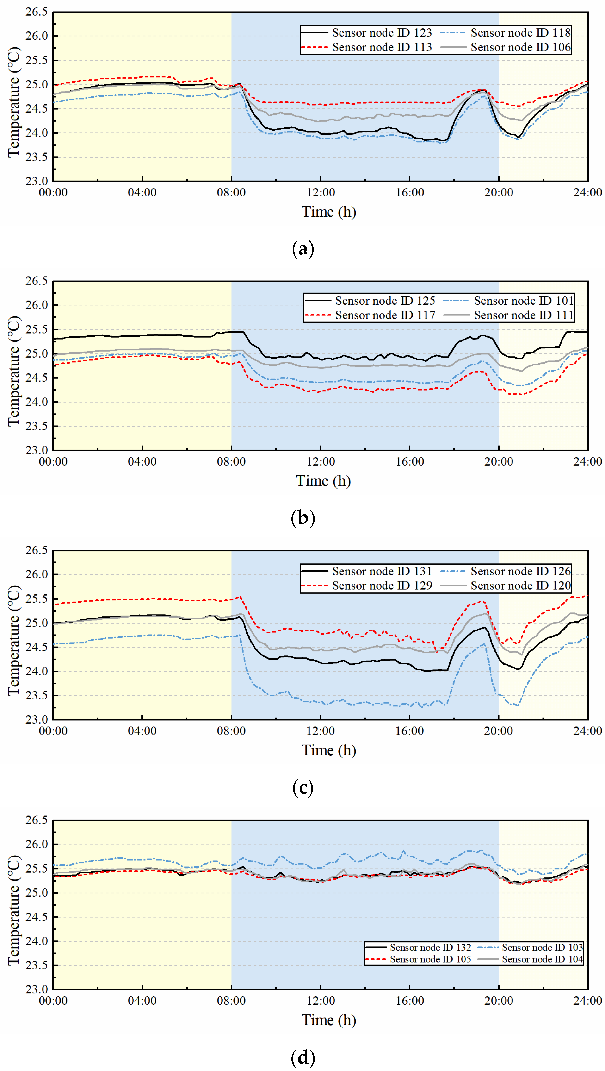
Figure 3 shows the temperature change of 16 sensor nodes in the four subzones of the space during one specific day, it reveals that the large space has uneven temperature distribution and local overcooling (lower than the set-point temperature 24.5 °C). The temperature gradually decreases to the temperature set point after the air-conditioning had been switched on at around 8:00 in the morning. It is interesting that the temperature has a significant fluctuation from 6:00 p.m. to 8:00 p.m., mainly because this space is a concourse and temporary area for study, there are a lot of moving students during this period of time, in addition, local students prefer to stay longer.

The measured historical temperature of each wireless sensor represents the historical change of temperature of the large space at that measurement point, the difference of monitoring data between different wireless sensors at the same moment can reflect the temperature difference in the horizontal direction. The maximum temperature difference in the horizontal direction of the space within this day occurs at 15:42 p.m., with a measured temperature of 25.8 for node 103 in the North zone, and a measured temperature of 23.35 °C in node 126 in the Middle zone. The horizontal temperature difference reaches 2.5 °C, which indicates the existence of local overcooling/overheating phenomenon in the large space. Furthermore, the temperature for node 126 in the Middle zone is always lower than the temperature of other nodes, while the temperature for node 103 in the North zone is always higher than the temperature of other nodes, which suggests the continued existence of local overcooling and overheating phenomenon in this large space for a long time. Similarly, humidity and CO₂ concentration also show the phenomenon of uneven distribution in space and time.

3. Data Reconstruction

3.1. Correlation Analysis of Sensor Nodes

One of the main starting points for reconstructing data is to ensure the continuity of the measurement data, since in the future control the site-measured wireless data can be directly integrated into a local controller. In a WSN-based monitoring system in buildings, one primary concern is the data transmission reliability, this is because the wireless signal transmission is not as reliable as the wired one, and the data received through WSN may suffer from various types of abnormality, typical abnormal data include data duplication, data loss and measurement outlier. Before reconstructing the data, duplicate data was removed according to the time when the data arrives, a modified z-score method was adopted to check the data continuity and remove the outliers. In this study, the authors mainly focused on how to reconstruct the missing data. Because the percentage of data loss of a single node is relatively large, only one of the sensor nodes will be selected for data reconstruction.

Correlation analysis is one of the methods to investigate the closeness of correlation between two variable factors, which is expressed by the following Pearson correlation coefficient equation [30]:

$$r=\frac{\sum \left({{\rm X}}_1-{\overline{{\rm X}}}_1\right)\left({{\rm X}}_2-{\overline{{\rm X}}}_2\right)}{\sqrt{\sum {\left({{\rm X}}_1-{\overline{{\rm X}}}_1\right)}^2{\left({{\rm X}}_2-{\overline{{\rm X}}}_2\right)}^2}}$$

(1)

where r is Pearson correlation coefficient, X₁ and X₂ are two variables, ${\overline{X}}_1$ and ${\overline{X}}_2$ are the average values of X₁ and X₂, respectively.

Each temperature measurement time-series from each sensor node in the WSN can be considered as an independent variable, and the correlation coefficients between each other can be calculated using Pearson’s formula. We select node 120 as the study target because it had less data missing, which can help make data reconstruction easier compared with the site measurement data. The correlation coefficient between the remaining 19 wireless sensors and this sensor is calculated to form a correlation coefficient linkage graph for this node, as shown in Figure 4. The data above the horizontal line in Figure 4 indicates the correlation coefficient between a sensor node and sensor node 120, and the ones below the horizontal line indicates the linear distance from sensor node 120. For example, the correlation coefficient between node 123 and node 120 is 0.629, and the line-of-sight distance is 19.09 m. Figure 4 illustrates that: (1) a total of 11 sensor nodes are highly correlated (|r| ≥ 0.8) with node 120, 7 sensor nodes are moderately correlated (0.5 ≤ |r| < 0.8) with node 120, and 1 sensor node is lowly correlated with node 120 (0.3 ≤ |r| < 0.5), which indicates that the correlation between node 120 and other sensors is relatively close. (2) The sensor nodes with strong correlation with node 120 have a certain pattern in terms of distance. The closer the node is to node 120 in terms of linear distance, the more likely it is to be highly correlated, and the farther the node is to node 120 in terms of linear distance, the more likely it is to be moderately or lowly correlated. (3) The sensor node 114 with strong correlation with node 120 is not closer in distance. For example, the correlation coefficient between node 114 and node 120 is larger than that between node 131 and node 120, but the line-of-sight distance between node 114 and node 120 is 18.26 m, and the line-of-sight distance between node 131 and node 120 is 12.30 m. It should be noted that the correlation coefficient of each node in the figure varies with the calculated data, and the correlation coefficient of each node will be different.

Based on the above analysis, it can be seen that the sensor nodes have different degrees of correlation with each other. Therefore, the correlation between sensor data can be used to select some sensor node data that are the most relevant to the sensor node with missing data rather than all sensor data as inputs (e.g., the most similar correlation coefficients to node 120 are node 125, 114, and 129), and then the data reconstruction can be performed, which can significantly reduce the computational complexity and estimation efficiency.

3.2. Multiple Linear Regression Model (MLR) Based on Correlation Analysis

Multiple Linear Regression (MLR), as a classical modeling method in multivariate statistical analysis, is widely used in research. MLR is obtained by linearly fitting the independent and dependent variables using the principle of least squares, and the contribution of each variable to the dependent variable can be obtained by observing the regression equation [31,32]. The contributions of the respective variables to the dependent variable can be obtained by observing the regression equation, and the fit magnitude of the MLR model can be evaluated by statistical regression methods such as coefficient of determination (R²) and Mean Square Error (MSE) [33].

A multiple linear regression model between the independent variable and the dependent variable y via n sets of observations k (x_k1, x_k2, …, x_km) can be obtained by the following equations [31,32].

$$\{\begin{array}{c}{y}_1=b_0+b_1{x}_{11}+b_2{x}_{21}+\cdots +b_m{x}_{m1}\\ y_2=b_0+b_2{x}_{12}+b_2{x}_{22}+\cdots +b_m{x}_{m2}\\ \cdots \cdots \\ y_n=b_0+b_n{x}_{1n}+b_2{x}_{2n}+\cdots +b_m{x}_{mn}\end{array}$$

(2)

b₀, b₁, …, b_m are m + 1 regression coefficients to be solved, and the regression equation is obtained by solving the regression coefficient estimates by the least squares method.

$$y_i=b_0+b_1{x}_{1i}+b_2{x}_{2i}+\cdots +b_m{x}_{mi}$$

(3)

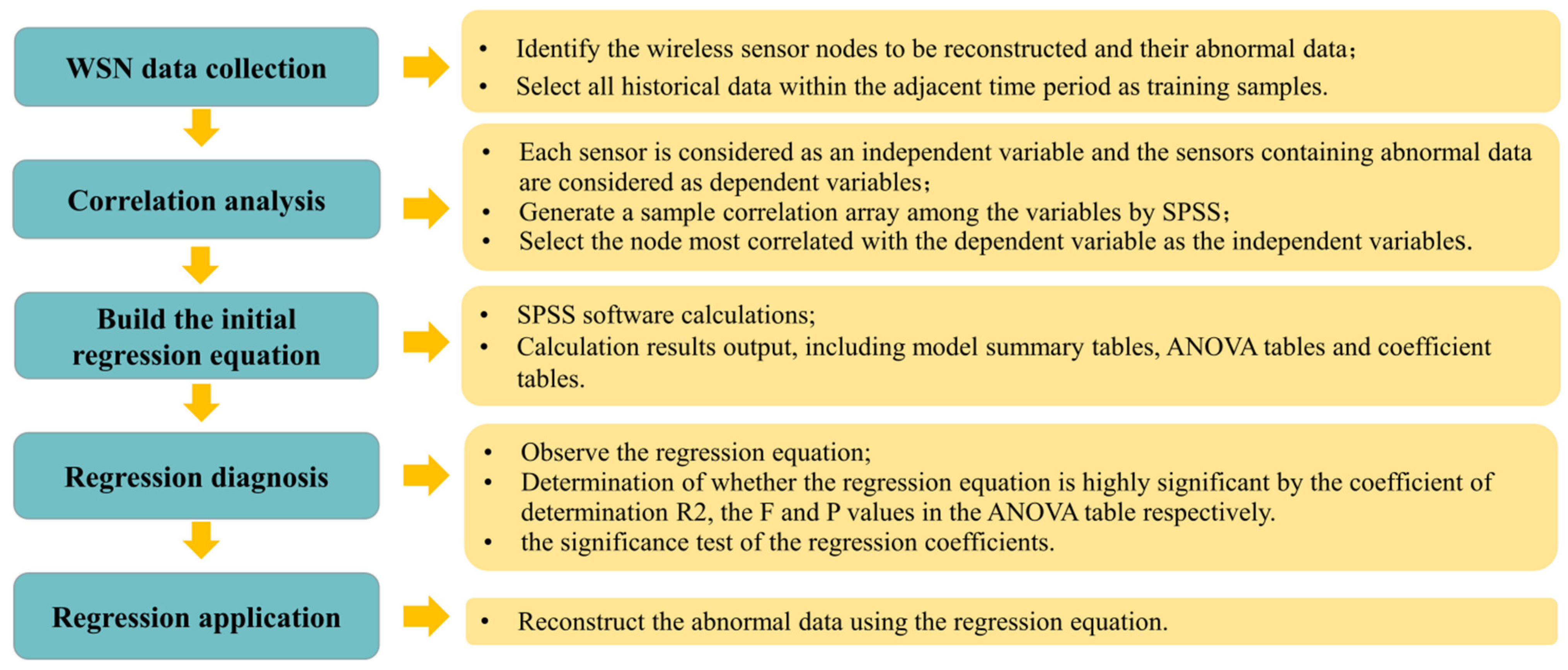
After obtaining the regression equation, the regression significance test is conducted to determine whether there is a linear relationship between the dependent variable y and the independent variable x₁, x₂, …, x_m. It mainly includes the significance of the regression equation and the significance test of the regression coefficients: the former is a test to determine whether there is linearity in the obtained regression equation, while the latter is a test to analyze the degree of influence of each independent variable on the dependent variable. The significance test allows analyzing the meaning of the regression equation and the contribution of the respective variables to the dependent variable. The steps of multiple linear regression using Statistical Product and Service Solutions (SPSS) software are given in Figure 5 [34,35].

In this study, multiple linear regression analysis was performed using SPSS software to reconstruct the abnormal data of a specific wireless sensor node. The correlation analysis between node 120 and other remaining sensors in the WSN network was performed based on the method introduced in aforementioned section. The sensor node with the higher correlation with node 120 was selected for MLR modeling, which can reduce the complexity of MLR calculation. The final regression equations for reconstructing the temperature, humidity, and CO₂ concentration data were determined as follows:

$$Y_{120,T}=0.395\times X_{125,T}+0.46\times X_{114,T}+0.131\times X_{129,T}+0.1$$

(4)

$$Y_{120,H}=0.358\times X_{125,H}+0.375\times X_{114,H}+0.299\times X_{129,H}-1.16$$

(5)

$$Y_{120,CO2}=0.433\times X_{125,CO2}+0.645\times X_{114,CO2}+0.090\times X_{129,CO2}+0.082$$

(6)

Y_120,T represents temperature data of node 120, X_125,T, X_114,T, and X_129,T represent temperature of nodes 125, 114, and 129, respectively; Y_120,H represents humidity data of node 120, X_125,H, X_114,H and X_129,H represent humidity of nodes 125, 114, and 129; Y_120,CO2 represents CO₂ of node 120, X_125,CO2, X_114,CO2, and X_129,CO2 represent CO₂ of nodes 125, 114, and 129, respectively.

3.3. Support Vector Regression Model

Vapnik et al. [12] proposed the Support Vector Machine (SVM) algorithm in the 1990s, which has gradually become the mainstream technique of machine learning. SVM is based on the principle of structural risk minimization and uses kernel functions to map linearly indistinguishable samples from low-dimensional mappings to high-dimensional feature spaces, and then constructs the optimal classification plane so that the total distance from each sample to the plane is minimized [36,37]. SVM is widely used in many fields such as prediction studies of time series, regression analysis, pattern recognition, and control because it can overcome the problems of ‘dimensional catastrophe’, local extreme, and small samples, and obtain a unique global optimal solution, which is called Support Vector Regression when solving regression problems [38].

For the given a sample data D = (x_i(j), y(j), i = 1, 2, …, M, j = 1, 2, …, N), x_i(j) is the jth sample of the ith variable, y(j) is the corresponding output value, N is the sample capacity. The basic idea of SVR is to map the sample X to a high-dimensional feature space (as shown in Figure 6a) by a nonlinear mapping function φ(x), and to perform linear regression analysis in this feature space, and then construct the optimal decision function y(x) in Equation (7). The output of SVR is a linear combination of intermediate nodes, each of which corresponds to a support vector, and its structure is shown in Figure 6b.

$$y\left(x\right)=w^T\phi \left(x\right)+b$$

(7)

$$\min \phi \left(x\right)={\frac{w}{2}}^2+C{{\displaystyle \sum }}_{i=1}^N\left|y\left(j\right)-\left[w^T\phi \left(x\left(j\right)\right)-b\right]\right|$$

(8)

φ(x) is the mapping function, w is the weight vector, and b is the bias, w and b can be calculated by Equation (8). C is the penalty factor to control the model loss w²/2 and the training model complexity. The kernel function is used to achieve a high-dimensional mapping feature space for the data, and the Lagrange equation is further introduced to solve Equation (8) to obtain the SVR output model results,

$$y\left(x\right)={\displaystyle \sum }\alpha \left(j\right)k{\left(x_j,x\right)}^{ }+b$$

(9)

where k(x_j, x) is the kernel function and α is the Lagrange multiplier.

In this paper, the above-mentioned principles are adopted to study the nonlinear relationship between the measurement time-series by one sensor node and others. A support vector machine regression model will be established to reconstruct the abnormal data. The kernel function of the support vector machine regression model in this paper employs the most commonly used Gaussian radial basis function kernel, and the parameter Gamma determines the high-dimensional feature space distribution of the data mapping, and the best combination of parameter Gamma and penalty factor C can be found by the grid method using cross-validation with the termination condition Epsilon set to 0.001.

3.4. Back Propagation (BP) Neural Network Model

In the mid-1980s, the Error Back Propagations Training algorithm was proposed, which solved the problem of learning the connection rights of the implicit layer of multilayer neural networks and performed a complete mathematical derivation [39]. The BP neural network has the ability of arbitrarily complex pattern classification and excellent multi-dimensional function mapping ability, which solves the heterogeneous or some other problems that cannot be solved by simple sensors [40]. The minimum value of the objective function is calculated using the gradient descent method [41,42].

The basic structure of BP neural network based sensor data reconstruction is shown in Figure 7. Given a training set D = (x_i(j), y(j), i = 1, 2, …, M, j = 1, 2, …, N), where the input layer contains m nodes, the implicit layer contains n nodes, and the output layer has one node. W_ih (i = 1, 2, …, m; h = 1, 2, …, p) is the weight between the i_th neuron in the input layer to the h_th neuron in the hidden layer, and W_ho (h = 1, 2, …, p; o = 1) is the weight from the h_th neuron in the hidden layer to the o_th neuron in the output layer, and θ_h (h = 1, 2, …, p) is the threshold of the h_th neuron in the hidden layer, σ₁ is the threshold of the output layer, X_i (i = 1, 2, …, m) is the I neuron of the input layer of the BP neural network, Y₁ is the neuron of the output layer of the BP neural network, Y_k is the expected output of the BP neural network, and e is the error between the expected output and the actual output of the BP neural network [42,43].

The input received by the h_th neuron in the hidden layer is α_h, the input received by the neuron in the output layer is β, see Equations (10) and (11), and b_h is the output of the h_th neuron in the hidden layer. It is assumed that the Sigmoid function is used in both the hidden layer and the output layer.

$${\alpha }_h={{\displaystyle \sum }}_{i=1}^m{w}_{ih}{x}_i$$

(10)

$$\beta ={{\displaystyle \sum }}_{h=1}^P{w}_{hj}{b}_h{}^{ }$$

(11)

For the training sample (x_k, y_k), the output of the output layer is noted by $\widehat{y}$, then the mean square error E_k of the BP neural network on (x_k, y_k);

$$E_k={\frac{1}{2}}^{ }{\left({\widehat{y}}^k-y^k\right)}^2$$

(12)

The BP algorithm is a type of iterative learning algorithm that uses generalized perceptron learning rules to update the parameters in each round of iteration. Moreover, the parameters are tuned in the direction of the negative gradient of the objective function based on a gradient descent strategy, with the goal of minimizing the cumulative error E on the training set.

$$E_{ }={\frac{1}{N}}^{ }{{\displaystyle \sum }}_{k=1}^N{E}_k=\frac{1}{2N}{{\displaystyle \sum }}_{k=1}^N{\left({\widehat{y}}^k-y^k\right)}^2$$

(13)

Hornik et al. proved that if a hidden layer contains a sufficient number of neurons, the neural network can infinitely approximate any continuous function with arbitrary accuracy [44]. Because of this powerful representation, self-learning and self-adaptive capability of BP neural networks, overfitting phenomenon often occurs, i.e., the training error continues to decrease while the test error keeps rising. However, the overfitting phenomenon can be effectively alleviated by adopting the two strategies of “early stop” and “regularization” [43].

In the model building of this paper, there are 19 neurons in the input layer, 1 hidden layer, and 10 neurons in the hidden layer, Mean Square Error is used as the objective function and gradient descent method is utilized to calculate the minimum objective function, the learning rate of the neural network is 0.1, and the termination condition Epsilon is set to 0.001, the detailed analysis results will be discussed in the next section.

3.5. Reconstructed Data Analysis

The experimental data used 1008 sets of actual measured data (each set of actual measured data contains 20 data) from 20 wireless sensor nodes during one week, it is divided into training set, validation set and test set for SVM and BP neural network model, and their distribution is shown in Figure 8. 1~720th sets of data (5 days) in training is for modeling, 721~864th sets of data (1 days) in validation are for verifying the effectiveness of the model, 865~1008th sets of data (1 days) in test are considered as test results to check the rationality of data distribution. It is noted that we did not follow the regular scaling law for the training-set, validation-set and test-set size ratio (usually 6:2:2), the actual ratio in this paper is 7:1.4:1.4. The reconstruction results are shown below. From the previous data loss analysis (Section 2), the data loss is less than 5 for most of time, thus linear interpolation can be employed in advance to replenish the lost data to guarantee data continuity, thus the selected training data are complete and continuous without outliers and missing data.

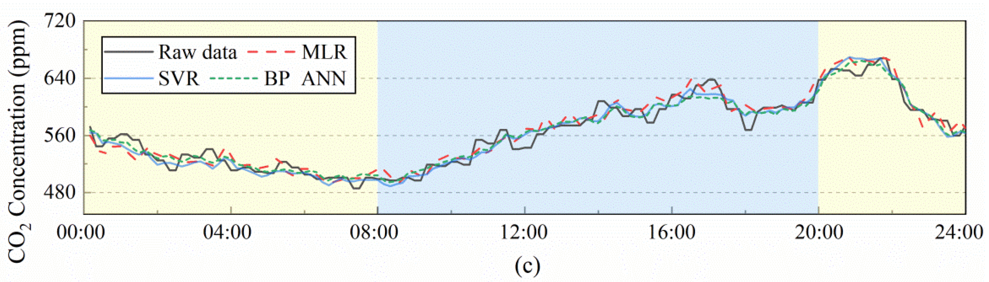
Figure 9 shows the fitted curves of the reconstructed data and the measured data by three algorithms. Although there are some deviations in the fit curves of the reconstructed data, the overall change trend is consistent, and the fit curves of the reconstructed humidity data have the highest coincidence with the measured data, followed by the temperature fit curve, the CO₂ concentration fitting curve was the worst. It indicates that the three algorithms have good accuracy in reconstructing temperature, humidity, and CO₂ concentration data.

$$R^2=1-\frac{{\sum }_{i=1}^M{\left(y^{\left(i\right)}-{\widehat{y}}^{\left(i\right)}\right)}^2}{{\sum }_{i=1}^M{\left(y^{\left(i\right)}-{\overline{y}}^{\left(i\right)}\right)}^2}$$

(14)

$$MSE=\frac{1}{M}{{\displaystyle \sum }}_{i=1}^M{\left(y^{\left(i\right)}-{\widehat{y}}^{\left(i\right)}\right)}^2$$

(15)

To further investigate the reconstruction accuracy of the three algorithms, R² and Mean Square Error are selected and their formulas are given in Equations (14) and (15), where M is the total number of samples, and y⁽ⁱ⁾, $\widehat{y}$⁽ⁱ⁾, $\overline{y}$ are the ith measured data, the ith reconstructed data, and the average value of the samples, respectively. The closer the R² is to 1 and the Mean Square Error is to 0, the better the model reconstruction is. 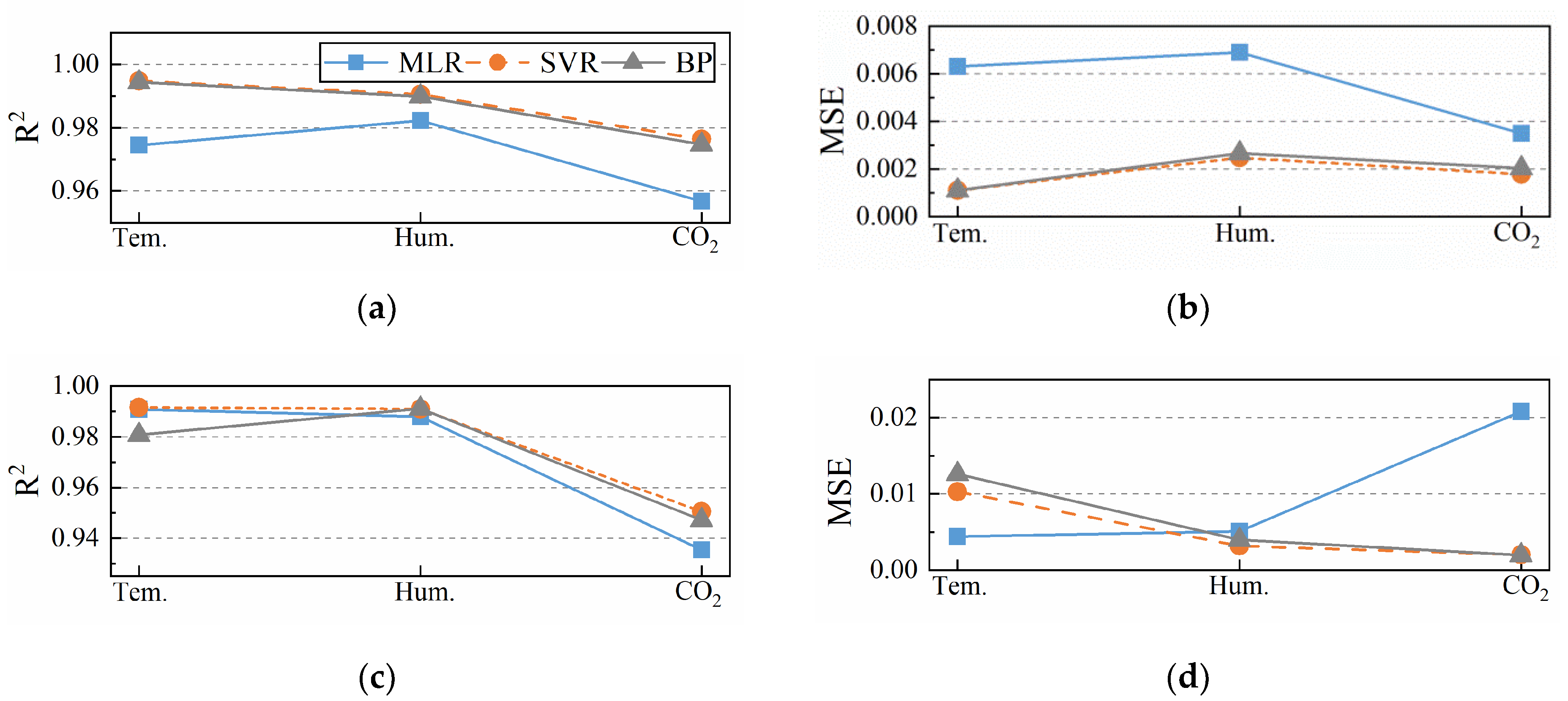It should be emphasized that since temperature, humidity, and CO₂ concentration have different units and magnitudes. Therefore, in the procedure of data preprocessing, the three data are normalized so that they are all distributed between 0 and 1. As an example to analyze the accuracy of the three algorithms in reconstructing temperature data, Figure 10 gives the specific performance of the three algorithms in reconstructing temperature data in the training and test sets. It can be seen that the performance of each model on the training and test sets is very close to each other, with no overfitting phenomenon. The R² based on the SVR model reconstruction is 0.9915, the MSE based on the MLR model reconstruction is 0.0044, and the R² and MSE based on the BP neural network model reconstruction are 0.9808 and 0.0126, and their performance is the worst in comparison with other methods. The results demonstrate that the accuracy of reconstructing temperature data based on SVR model and MLR model is higher than that based on BP neural network model. It has different performance in reconstructing temperature, humidity and CO₂ with exactly same algorithm, Figure 10c shows the accuracy of reconstructing the data based on BP algorithm is humidity, temperature, and CO₂ concentration in order. The accuracy of reconstructing the same data based on different algorithms also varies. Figure 10d reveals the highest accuracy of reconstructing temperature data is MLR algorithm, followed by SVR and BP algorithm. Accuracy is not the only index to measure the superiority of the algorithm. From the perspectives of program complexity, computing speed and difficulty in obtaining input conditions, MLR is the most suitable one of the three methods.

4. TRNSYS Modeling and Control Simulation

Because rooms are often over-conditioned needlessly, without properly dealing with the temperature uneven distribution, the performance of the temperature control may deteriorate and energy may be wasted. Therefore, the current control system needs to be retrofitted and a new zonal demand control strategy was proposed. The air conditioning system of the four subzones is modeled using TRNSYS, TRNSYS is a very popular commercial software that can be used in HVAC control field. The detailed building model of this large space is created by Type 56, as shown in Figure 11. Four subzones are connected with 4 regular PID (Propotional, Integral, Derivative) controllers to control their corresponding subzone with suitable airflow rate based on the subzone temperature set-point. CONTAM [45], developed by the U.S. national institute of standards and technology, is a multi-zone indoor air quality and ventilation analysis program designed to assist in identifying airflow, pollutant concentrations, and occupant exposures within a building. The application of CONTAM to predict airflow and pollutant transport was validated by many researchers [46,47,48]. CONTAM calculates infiltration and exfiltration airflow between interior areas of a building and the outdoors, airflow from room to room, and airflow from ventilation systems. These airflows are caused by pressure differences resulting from driving forces, including fans in mechanical ventilation systems, wind pressure acting on the exterior of the building, and buoyancy effects induced by temperature differences between zones, including outdoors. The building model separated into four subzones with a virtual boundary, for control applications, the airflow may interact between the virtual boundaries. Thus, it is important to calculate the airflow during every control time intervals. Fortunately, CONTAM can be competent to this task. The four subzones of the building temperature are connected to the CONTAM module, which uses these external input data to calculate the airflow exchange between the rooms and the outdoor environment as well as the airflow exchange between the rooms. The airflow exchange (airflow coupling) between the zones generated by CONTAM is connected to the rooms as input, and the mechanical ventilation of the system with the air conditioner synergistically affects the room temperature. 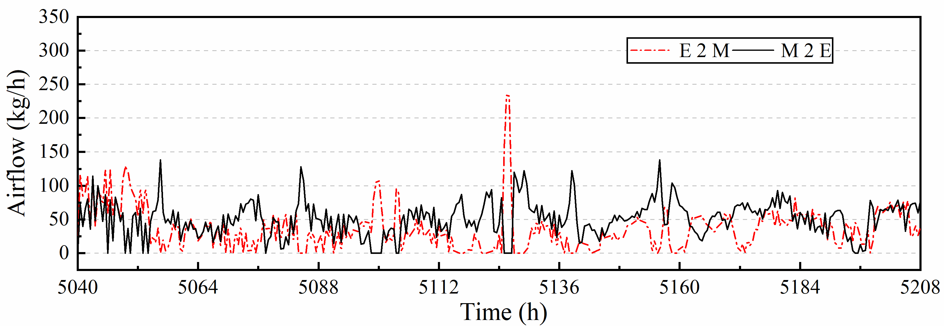The schematic diagram of airflow exchange in each subzone is shown in Figure 12, the interaction between the zones is marked with blue arrows in the figure. For example, M to E represents the airflow from Middle zone to East zone through virtual boundary.

4.1. Description of Three Control Modes

More wireless sensors can be deployed in a large space for precise measurements, which can be used as input to the temperature controller for more accurate zonal temperature control. Although the implementation of a BACnet-ZigBee gateway is impractical, the feasibility of wireless sensor-based temperature control will be discussed in advance. Here three control modes are used for comparison purpose:

• The traditional single-input-single-output (SISO) control: the use of only one temperature sensor to synchronously control the entire large space, the temperature sensor is usually located at the return air outlet, the airflow rate is delivered to the space evenly by the air terminals (e.g., square ceiling diffuser). This is the current temperature control mode for this large space. The baseline model or the benchmark model introduced here is for energy consumption comparison purpose.
• Zonal temperature control: The whole space is separated into four individual subzones, with each subzone can be independently controlled to its corresponding zonal set-point temperature (zonal set-point temperature may varies with different subzones for energy conservation).
• Zonal demand control: Based on the zonal temperature control, the following two aspects were considered: (i) The relationship between room set-point temperature and room load is shown in Figure 13. The temperature set-point changes with the load, when the load is on a small scale, the temperature set-point increases appropriately, when the load exceeds a certain value, for example 2 kW, the temperature set-point decreases accordingly; (ii) the airflow coupling between virtual boundaries are considered and calculated by CONTAM program.

The cooling load mainly depends on the number of mobile people inside, however it is very difficult to measure indoor loads directly. Alternatively, the real cooling load for consecutive weeks of the large space can be calculated by parameters such as air supply temperature, average zonal temperature from the wireless sensor nodes, and air supply flow rate, as shown in Figure 14. Interested readers may find more information in reference [17]. According to the actual use of the air conditioner in this area, the real load calculated is from July 1 to July 7, which is equivalent to the setting time of TRNSYS software: 5040 h~5208 h. From Figure 14 it can be seen that except for the north area, the peak load is about 5.59 kW and the average load is 4.63 kW. The load in West is smaller compared with the load in East and Middle, with a maximum value of about 4.85 kW and an average load of 2.37 kW. The load in the North zone is basically the same as the load in the West zone in the morning and evening, but in daytime the load in the North zone is significantly lower than the load in the West zone since this subzone is a corridor area with people rarely stay. The load change curve basically reflects the obvious characteristic of uneven distribution of the load in large spaces. Using the measured load in Figure 14 as input, the air conditioning system of the above three control strategies was modeled and controlled with TRNSYS and CONTAM program respectively.

4.2. Simulation Results

Figure 15 shows the temperature response curves for the four subzones. It can be seen that the temperature in all three rooms except the East subzone is subcooled (below the set-point temperature: 24.5 °C). The reason is the input temperature sensor of the conventional control is located in this subzone. Actually, in TRNSYS, the subzone can be only seemed as one temperature node, so the control receives feedback only based on the temperature of this node, not the temperature of the whole large space. Since the load in the East area is greater than the other three subzones, and the air supply is delivered evenly into the entire large space, the supply airflow rate only meets the load in the subzone with the largest load, it is unavoidable to cause overcooling in other subzones. Similarly, if the East area load is the smallest, it will inevitably result in the overheating phenomenon for the other subzones, if the East area load is between the maximum and minimum of the four regional load, it may lead to some subzones to be overheated and some other subzones to be overcooled.

The zonal temperature control is shown in Figure 16 with four subzones has the same temperature set-point 24.5 °C. The temperature of all four subzones fluctuates between 24.25 °C and 24.9 °C. The temperature in four subzones is controlled well, and the overheating and overcooling phenomena was eliminated. From the simulation results, it can be seen that the independent control of zoning can solve the problem of overcooling and overheating in the virtual zones. Although the indoor thermal comfort is improved, the independent zonal control is not necessarily energy-saving, especially when the load in the area is smaller than other areas, the fan energy consumption can be reduced by appropriately increasing the set-point temperature. Furthermore, in TRNSYS, the division of this space is separated and seemed to be the solid walls, while the actual division of the space is without physical partitions, the air exchange between subzones should be taken into account since it can interfere the temperature control, thus the simulation conducted here is inconsistent with the reality.

The TRNSYS model was modified based on the above zonal demand control, CONTAM program was added to this model to calculate the air coupling effect between subzones, thus zonal demand control can be achieved with temperature setting value changes with load accordingly. As shown in Figure 17, the temperature of the 4 subzones fluctuates continuously with different setting values, with a maximum of 26.75 °C and a minimum of 24.5 °C. The temperature between subzones in the TRNSYS model interacts with each other since the heat mass exchange between zones is being considered in the TRNSYS model. Therefore, the results of joint control by TRNSYS and CONTAM are more reliable and more realistic. Since the variable temperature setting is different from the fixed set-point, the set-point temperature of each subzone is basically different at every moment in the case of variable temperature setting mode, it will cause a greater temperature difference between different subzones, which leads to a more intense airflow and accelerates the heat mass exchange between subzones, and the disturbance is more intense.

Figure 18 shows the airflow exchange calculated by CONTAM program between East and Middle, it means the airflow via virtual boundaries can be mixed with each other. For example, in East subzone, the airflow is not only from the air terminals but also from its adjacent subzone: the Middle. It is noted there are 10 interactions of air exchange in this case which is not shown in this figure. The exchange between zones is equivalent to an external disturbance which has an impact on the conventional PID controller, hence room temperature control experiences a large fluctuation. That’s why the north subzone experienced a sharp temperature decrease in control respond since it interacts with the three subzones, see Figure 17. The traditional PID control system used in this model has poor anti-interference capability, which can be solved by feedforward compensation control or other control algorithms.

Fan energy consumption was listed in

Table 2. Fan energy consumption with three control strategies.

Control Strategies	SISO Control (Benchmark)	Zonal Temperature Control	Zonal Demand Control
Room set-point	24.5 °C	24.5 °C	24.5–26.5 °C
Fan energy consumption	420.4 kWh	370 kWh	343.5 kWh

. For benchmark control, the weekly energy consumption by the fan is 420.4 kWh with room set-point 24.5 °C, fan power consumption for Zonal temperature control strategy is reduced to 370 kWh, which achieved 12% of energy savings compared to the benchmark model. For zonal demand control, the fan energy consumption is further reduced by 18% due to the variable temperature settings with respect to the benchmark model.

5. Discussion and Conclusions

In this study, a wireless sensor network has been constructed to monitor the temperature, humidity and CO₂ in a selected large indoor space with the purposes of improving the temperature control for energy saving as well as improving thermal comfort.

Due to various uncertainty factors, data loss, data duplication, data abnormalities and other problems may occur during data transmission, data loss is a common phenomenon in the operation of the wireless network. Firstly, the data loss rate was analyzed in a typical summer month. Twenty sensors collected a total of 74,880 temperature data with an average of 3744 data collected by each node. The number of missing data was 639 with an average loss rate of 0.85%. It is found different wireless sensor nodes have different data loss rates, No. 116 has the largest number of data loss, accounting for 10.26%, followed by node No. 129, 123, 111 and 120, and the rest of the nodes have less than 5 data loss.

Secondly, the daily and monthly data of temperature, humidity and CO₂ concentration was analyzed and summarized. Uneven distribution of temperature, humidity and CO₂ was observed, it is found the temperature in horizontal breathing level can be reached to 2.5 °C, which indicates the existence of local overcooling/overheating phenomenon in the large space for the current temperature control system, consequently, thermal comfort is not guaranteed.

Thirdly, from the point of view of temperature control, the wireless data will be employed as the input of the wired control system, thus the wireless measurement data must be reliable and continuous, since the input data has a significant impact on the operation and monitoring of the control system, so it is much crucial to reconstruct the lost data to ensure the system operated stably. Three algorithms for reconstructing data, namely multiple linear regression, Support Vector Regression and Back Propagation neural network, have been implemented and compared. The results demonstrate that the accuracy of reconstructing temperature data based on Support Vector Regression model and multiple linear regression model is higher than that based on BP neural network model. From the perspective of program complexity, computing speed and difficulty in obtaining input conditions, multiple linear regression is the most convenient of the three methods.

Finally, the feasibility of wireless sensor-based temperature control has been discussed in this paper as well. More wireless sensors can be deployed in a large space for precise measurements, which can be used as input to the temperature controller for more accurate zonal temperature control. Based on the monitored parameters, a multi-zone demand control model has been established on a TRNSYS-CONTAM joint-control platform to alleviate the phenomenon of overcooling/overheating for this large indoor space. The airflow exchanges across the virtual boundaries have been considered (it was calculated by an external program CONTAM) as well. Three control modes have been conducted: the benchmark model (the current conventional temperature Single-Input-Single-Output control model), the zonal model and the proposed zonal demand model. The simulation results showed the zonal demand model could alleviate the over-cooling or over-heating phenomenon in conventional temperature control. Thermal comfort performance was also improved by considering the zonal temperature demand. Moreover, it contributed to 18% reduction in fan power consumption compared to the benchmark model.

Limitations and outlook: The authors did not consider a larger sample space for the training set, only one week of data was selected as the training set in this paper. The meta parameters of Support Vector Regression and Back Propagation neural network methods are set by default, the effect of meta-parameters on data reconstruction results is not taken into account. The control simulation in this paper is conducted by simulation and not experimentally verified. Future work will focus on optimizing the data more efficiently, as well as enabling the integration of wireless data and control.