
Theoretical Impact of Building Façade Thickness on Daylight Metrics and Lighting Energy Demand in Buildings: A Case Study of the Tropics


Abstract
:1. Introduction
2. Concept
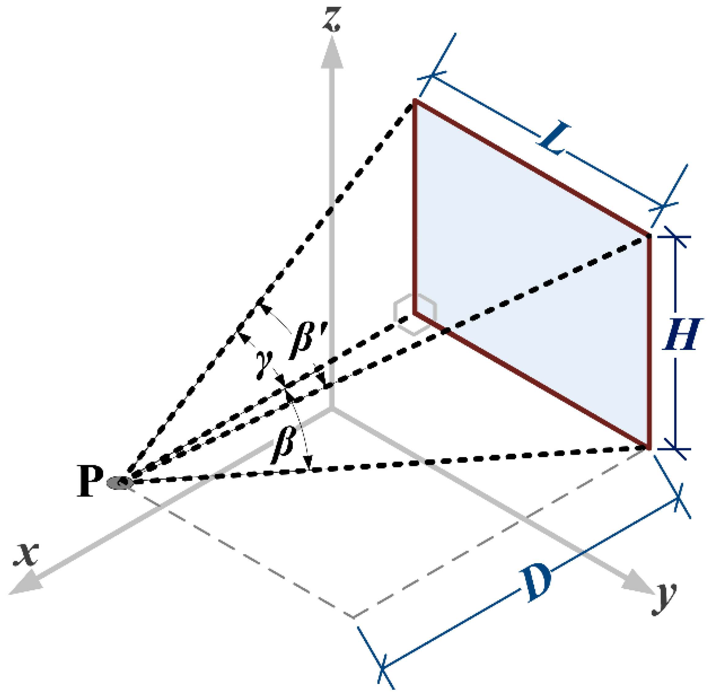
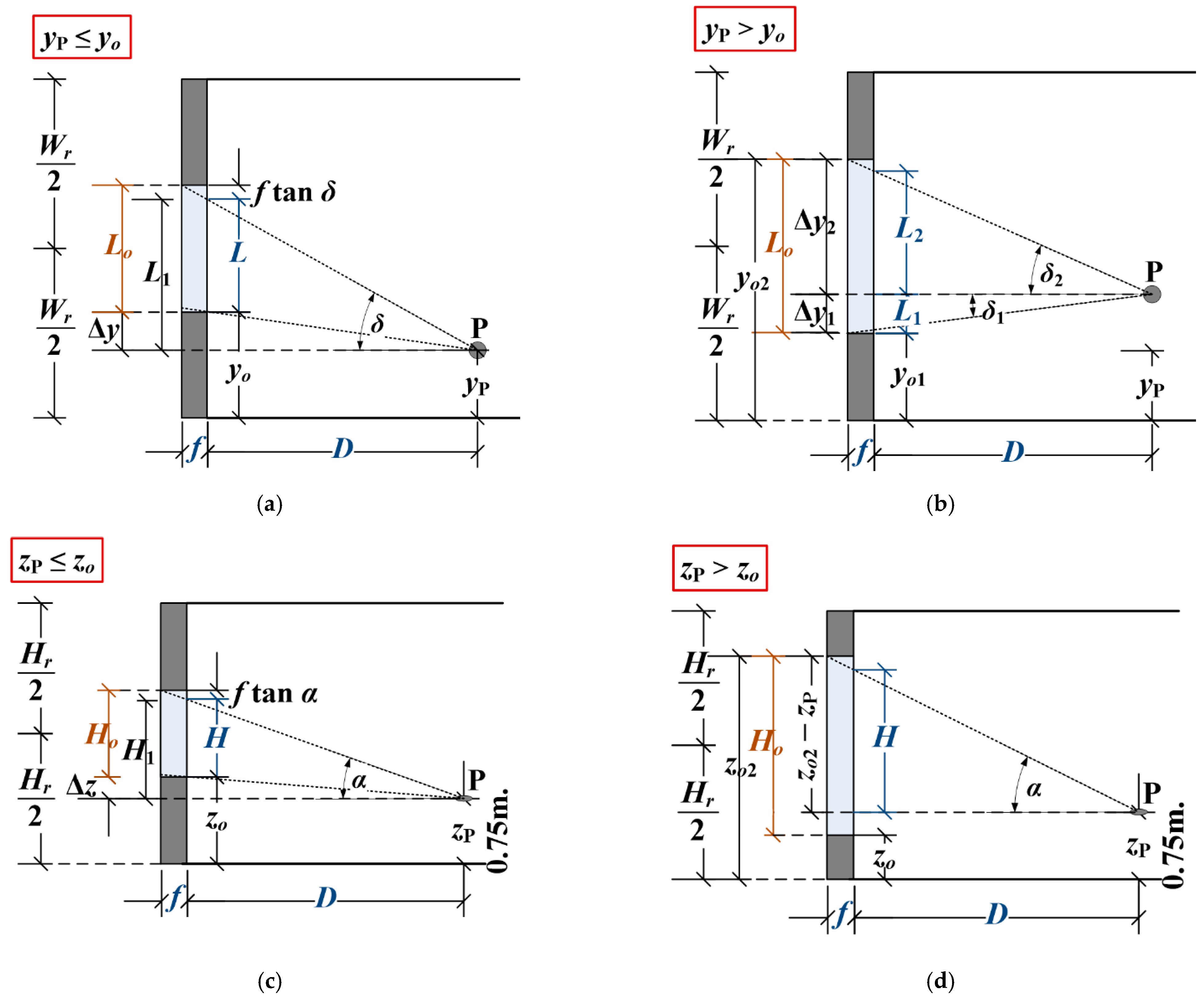
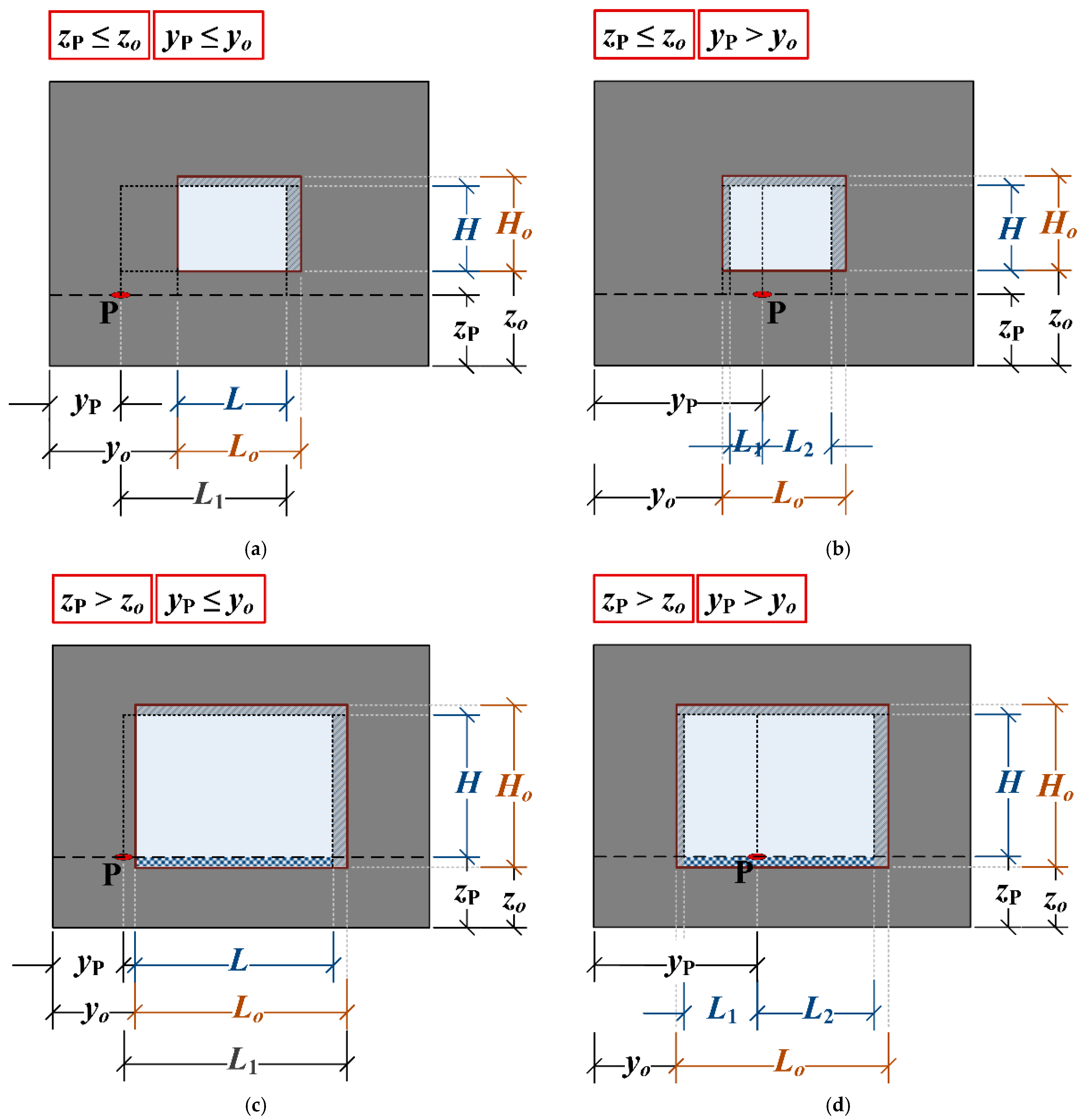
2.1. Sky Component
- (1)
- (2)
- (3)
- (4)
2.2. Externally Reflected Component
2.3. Daylight Factor
2.4. Climate-Based Daylight Metrics
- (1)
- Daylight autonomy, 300 lx threshold (referring to the LEED v4.1 recommendation [40]) (DA300):
- (2)
- Useful daylight illuminance, autonomous (100–2000 lx, i.e., the original range proposed by [41]) (UDI-a):
- (3)
- Useful daylight illuminance, autonomous (300–3000 lx, i.e., the new range proposed by [42]) (UDI-a′):
- (4)
- Useful daylight illuminance, exceeded (>2000 lx, i.e., the original range) (UDI-e):
- (5)
- Useful daylight illuminance, exceeded (>3000 lx, i.e., the new range) (UDI-e′):
2.5. Annual Lighting Energy Demand
3. Methods
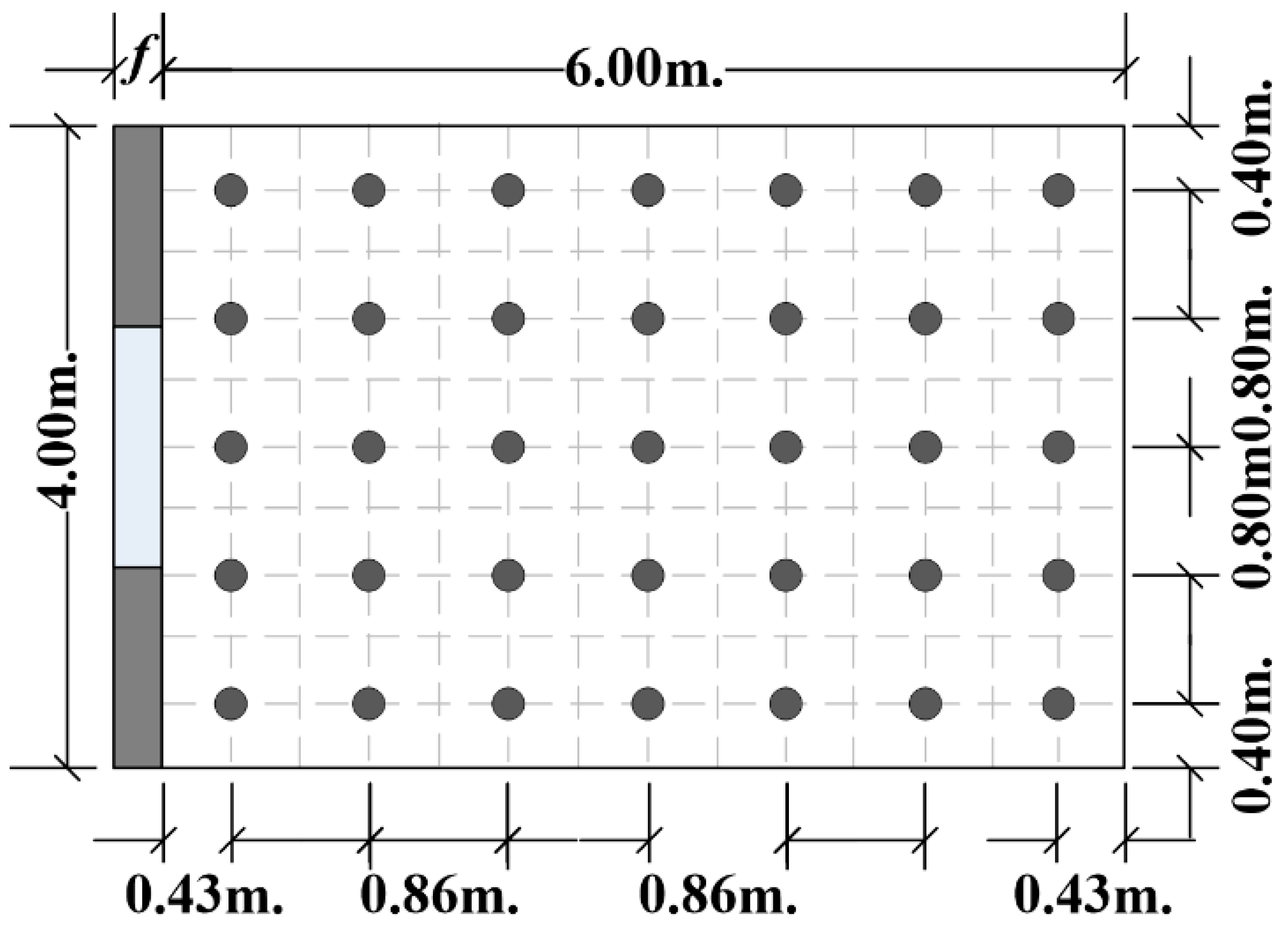
3.1. Room Settings
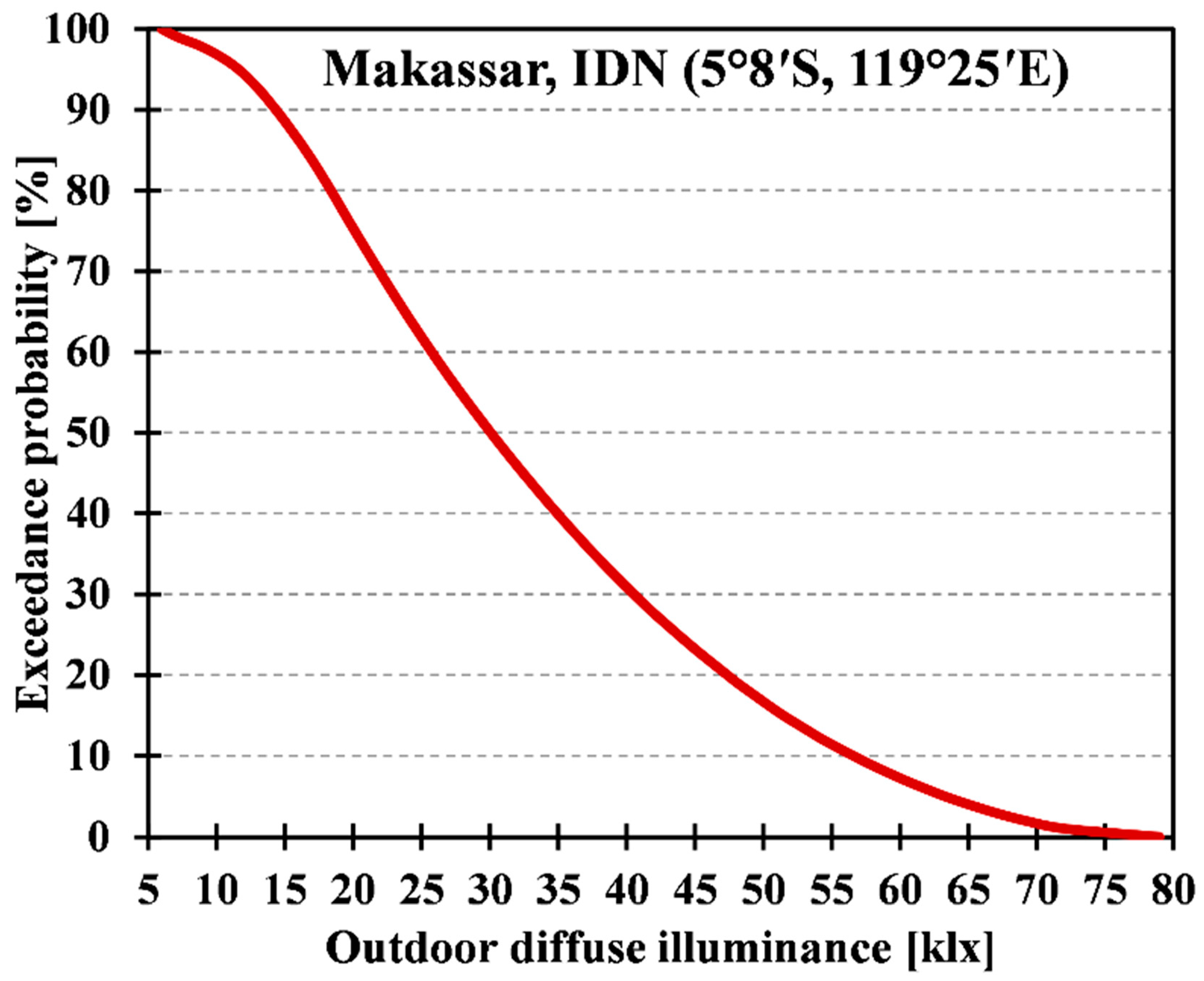
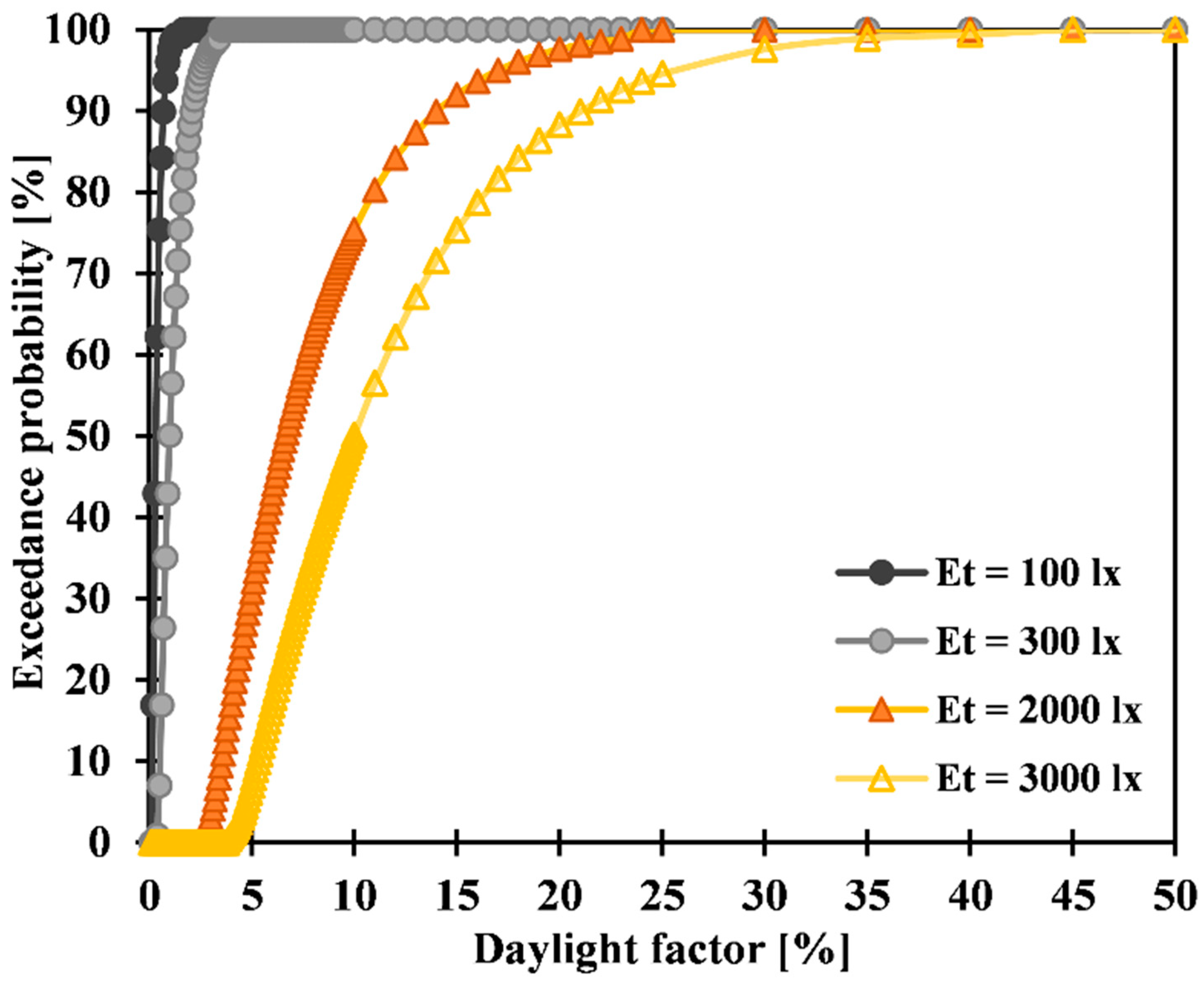
3.2. Annual Daylight Profile
3.3. Sensitivity and Uncertainty Analyses
- (1)
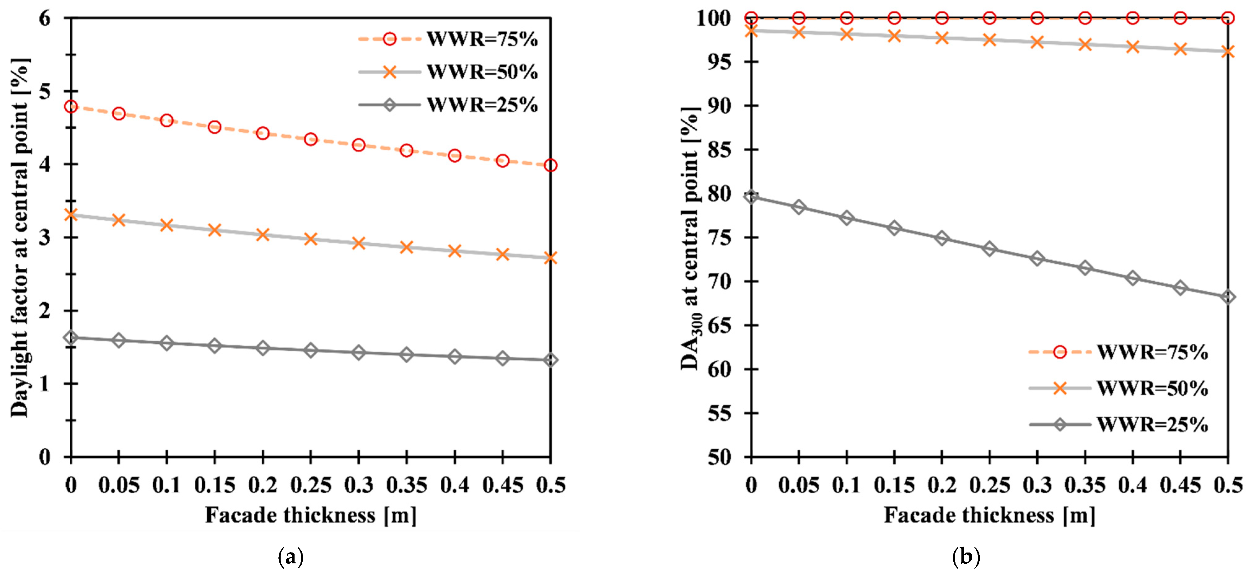
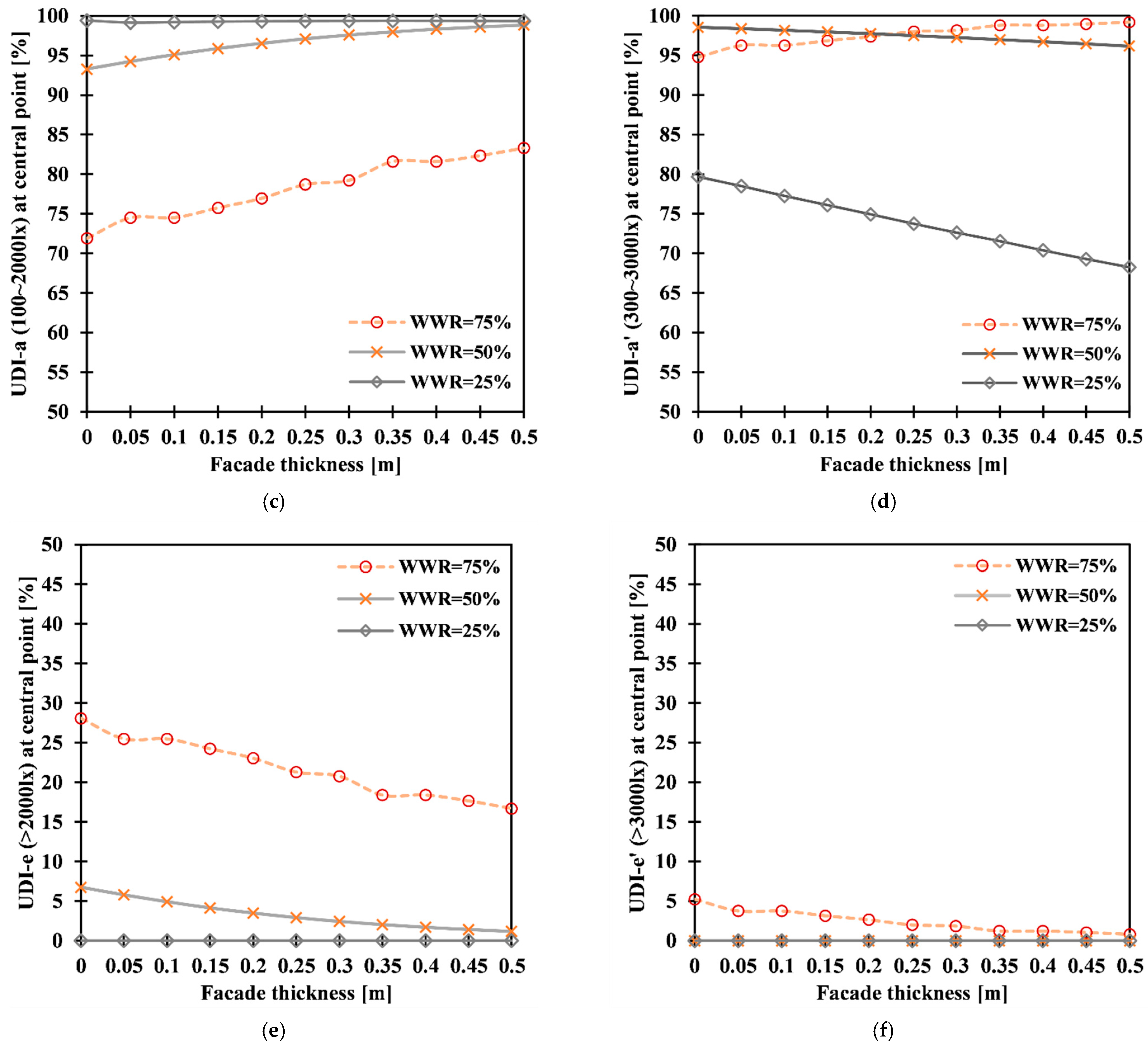
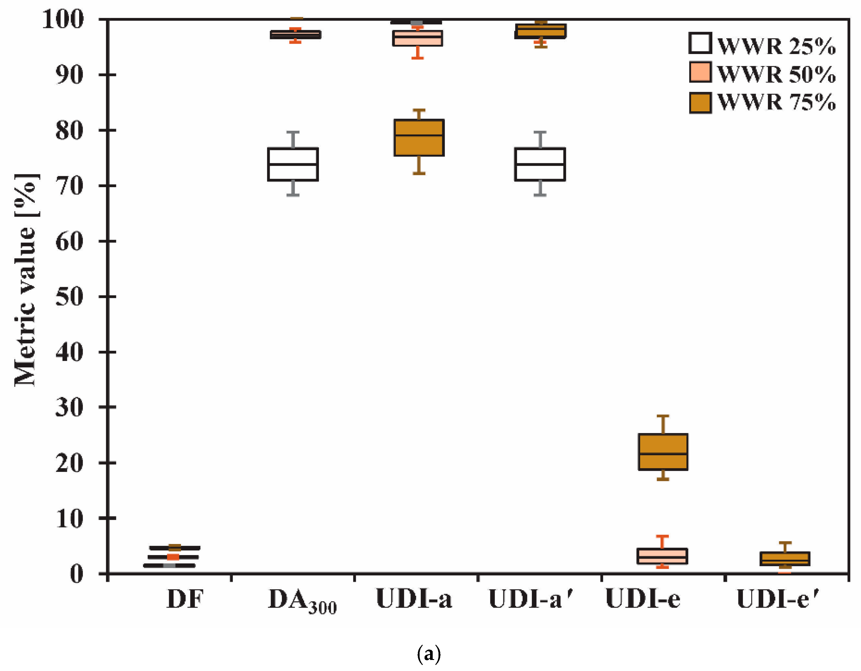
- Metrics at the central calculation point (cf. Figure 4), which include: DF, DA300, UDI-a, UDI-a′, UDI-e, and UDI-e′.
- (2)
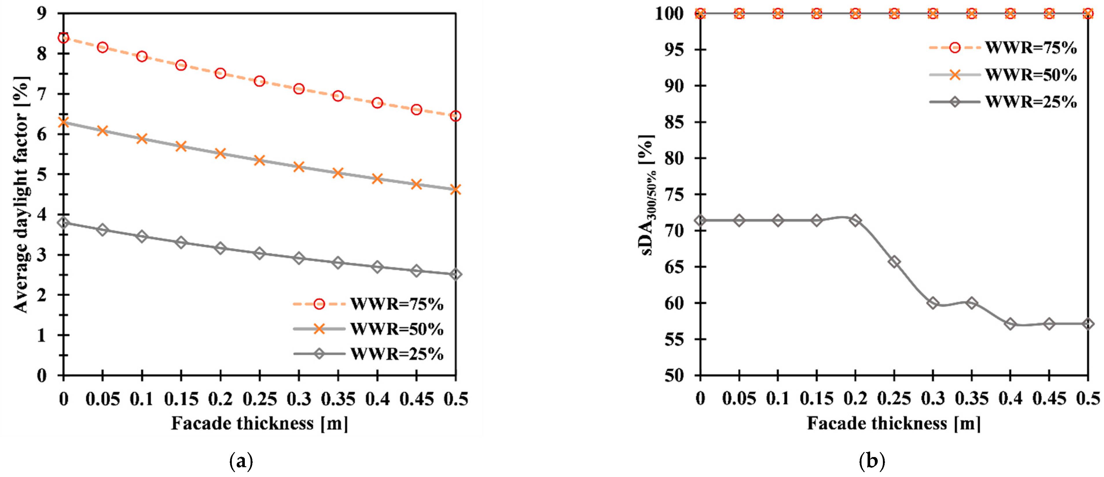
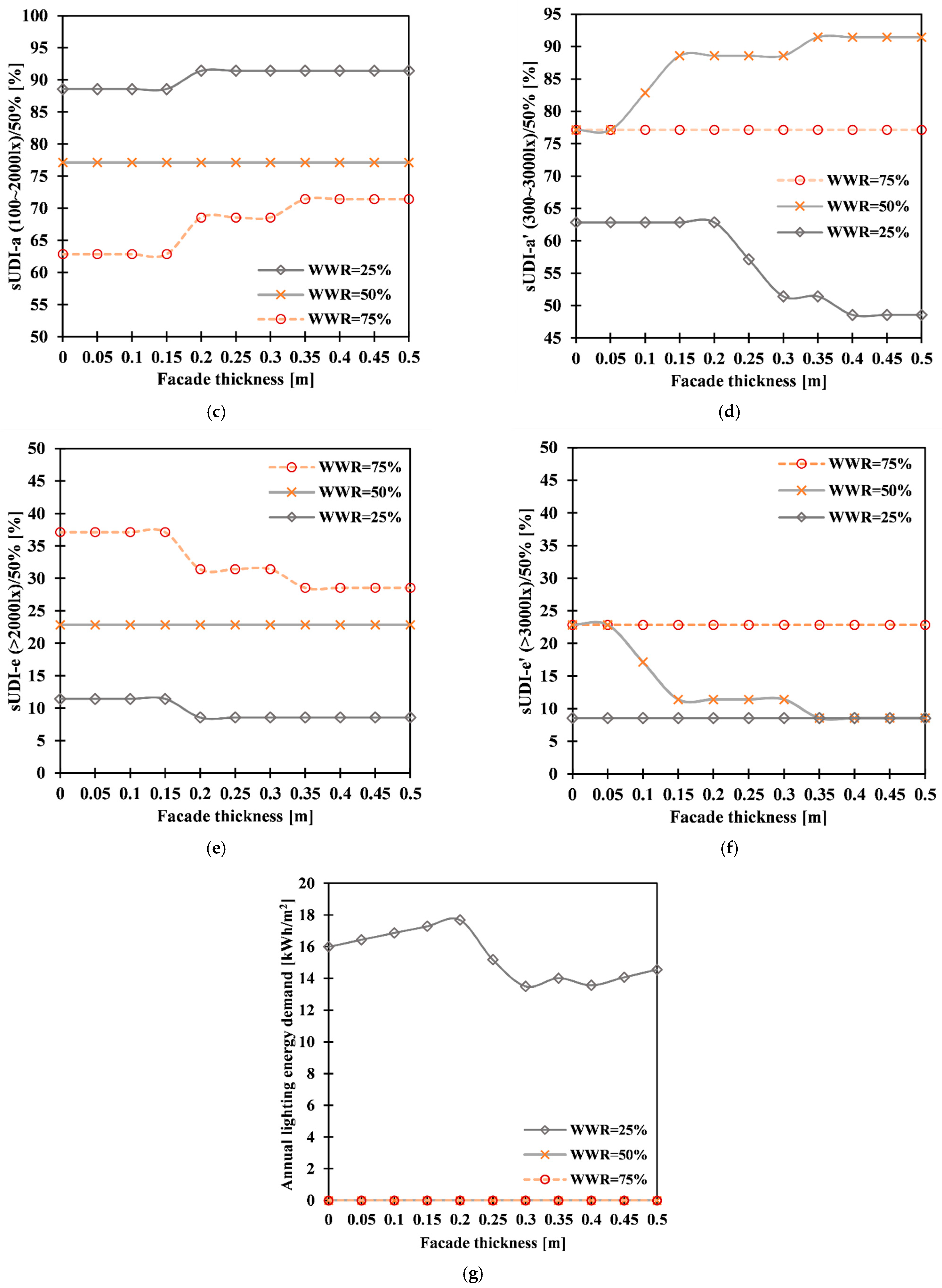
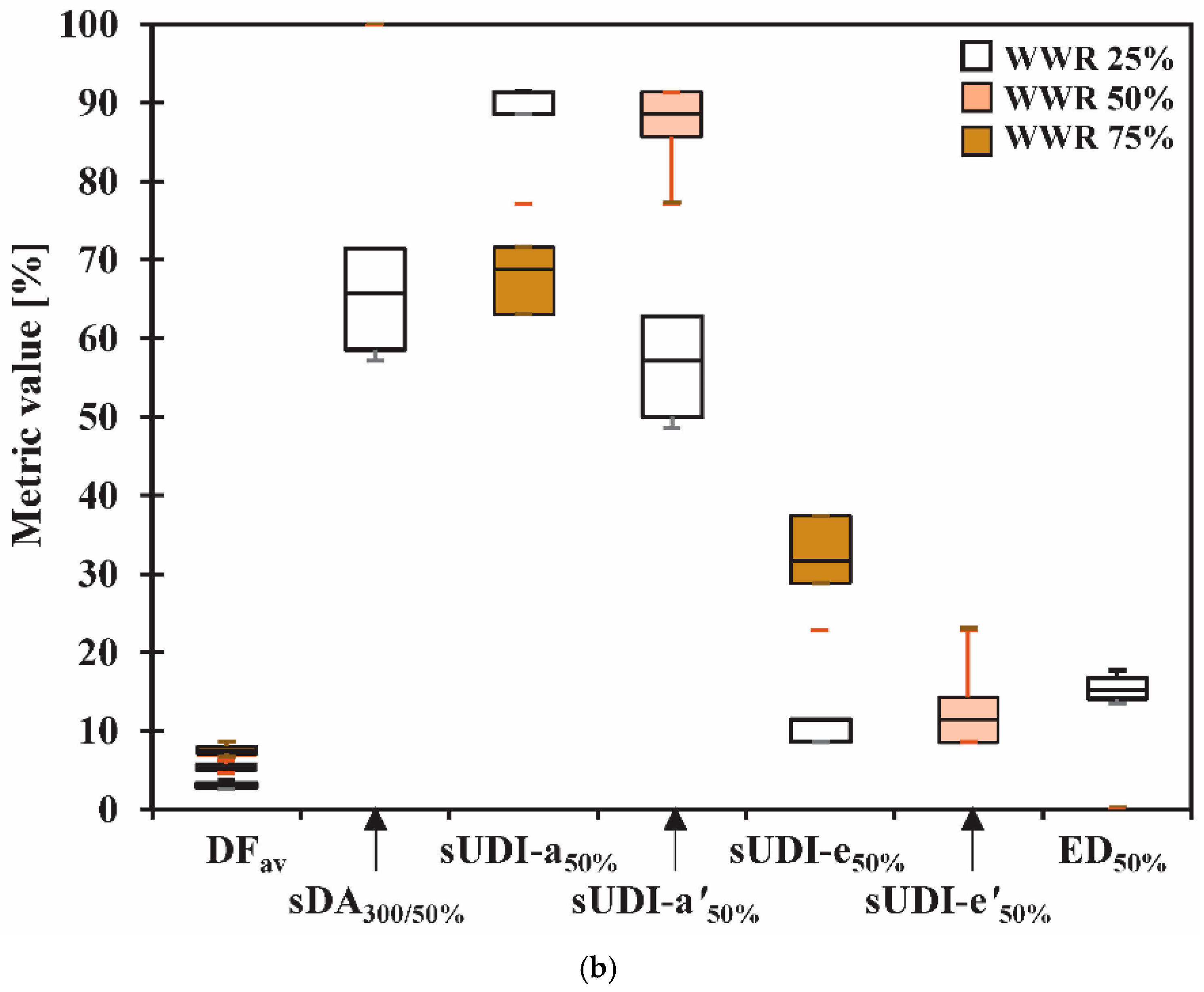
- Metrics for the entire room, based on all calculation points in Figure 4, which include: DFav, sDA300/50%, sUDI-a50%, sUDI-a′50%, sUDI-e50%, sUDI-e′50%, and ED50%.
4. Results
4.1. Sensitivity Analysis
4.2. Uncertainty Analysis
5. Discussion
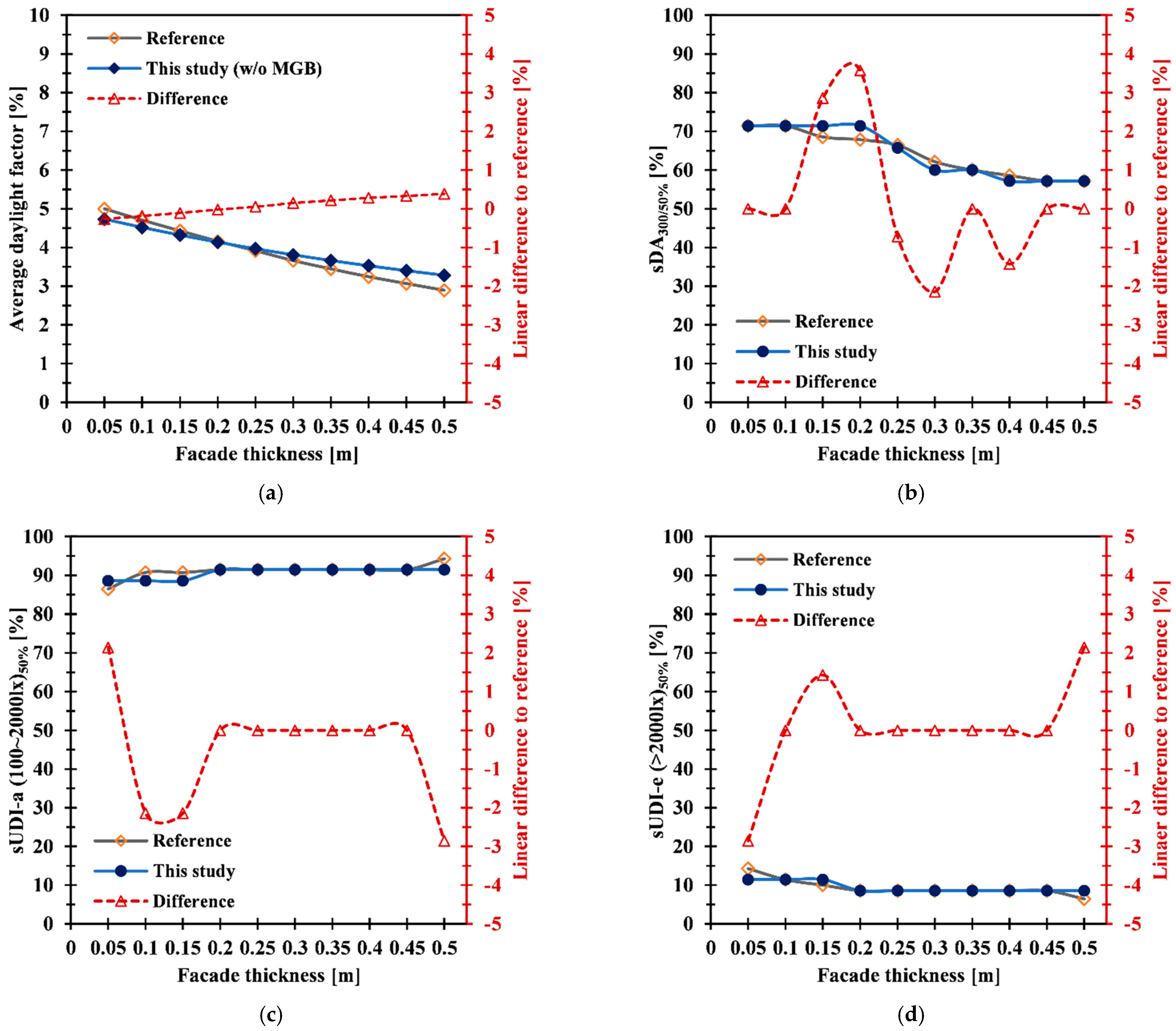
5.1. Inter-Model Comparison
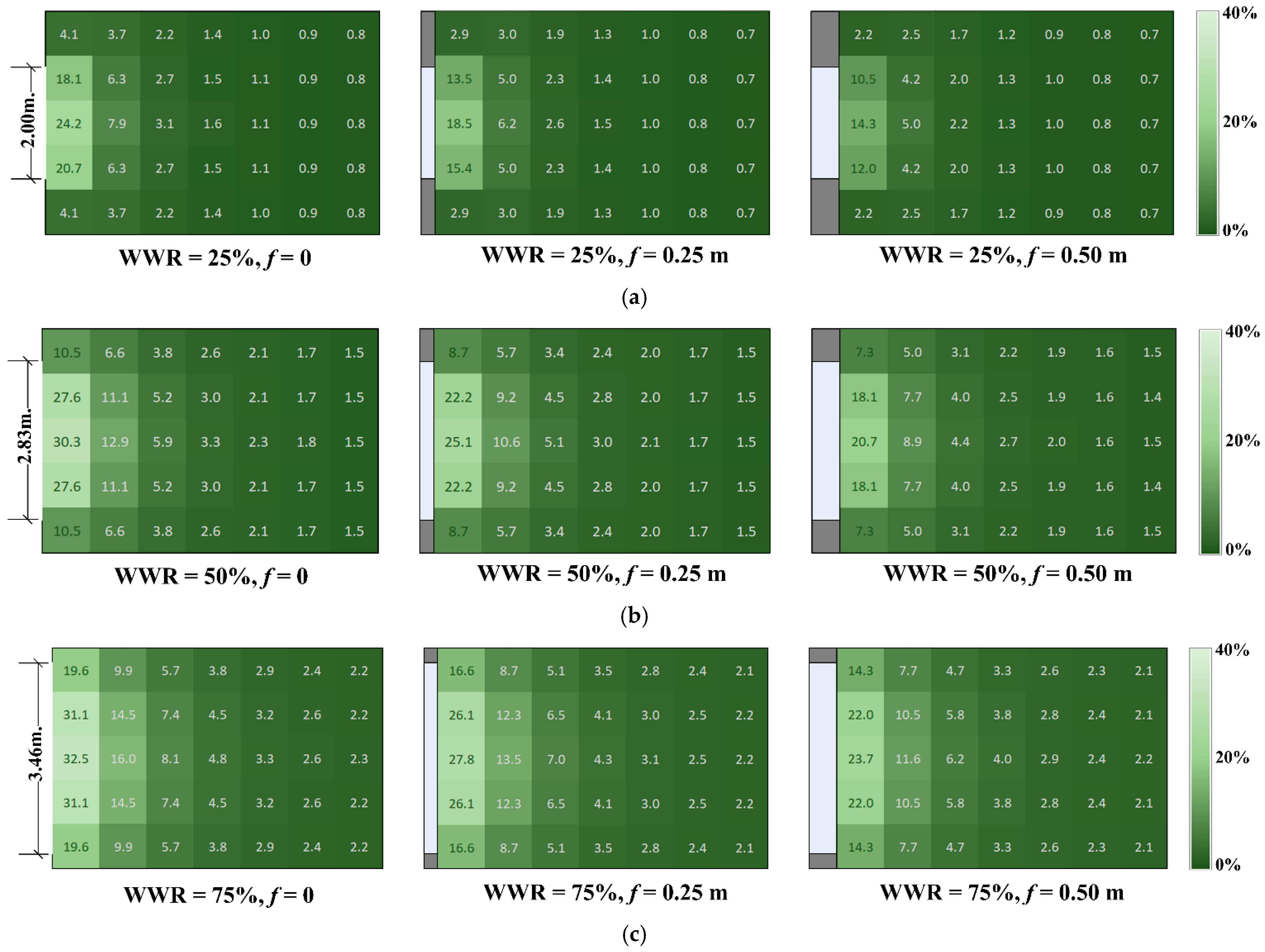
5.2. Spatial Distribution
5.3. General Discussion
6. Conclusions
Author Contributions
Funding
Institutional Review Board Statement
Informed Consent Statement
Data Availability Statement
Conflicts of Interest
References
- Bluyssen, P.M.; Aries, M.; van Dommelen, P. Comfort of Workers in Office Buildings: The European HOPE Project. Build. Environ. 2011, 46, 280–288. [Google Scholar] [CrossRef]
- Aries, M.B.C.; Veitch, J.A.; Newsham, G.R. Windows, View, and Office Characteristics Predict Physical and Psychological Discomfort. J. Environ. Psychol. 2010, 30, 533–541. [Google Scholar] [CrossRef]
- Aries, M.B.C.; Aarts, M.P.J.; van Hoof, J. Daylight and Health: A Review of the Evidence and Consequences for the Built Environment. Lighting Res. Technol. 2015, 47, 6–27. [Google Scholar] [CrossRef]
- Alzoubi, H.; Al-Rqaibat, S.; Bataineh, R.F. Pre-versus Post-Occupancy Evaluation of Daylight Quality in Hospitals. Build. Environ. 2010, 45, 2652–2665. [Google Scholar] [CrossRef]
- Lim, G.-H.; Hirning, M.B.; Keumala, N.; Ghafar, N.A. Daylight Performance and Users’ Visual Appraisal for Green Building Offices in Malaysia. Energy Build. 2017, 141, 175–185. [Google Scholar] [CrossRef]
- Jamrozik, A.; Clements, N.; Hasan, S.S.; Zhao, J.; Zhang, R.; Campanella, C.; Loftness, V.; Porter, P.; Ly, S.; Wang, S.; et al. Access to Daylight and View in an Office Improves Cognitive Performance and Satisfaction and Reduces Eyestrain: A Controlled Crossover Study. Build. Environ. 2019, 165, 106379. [Google Scholar] [CrossRef]
- Davoodi, A.; Johansson, P.; Henricson, M.; Aries, M. A Conceptual Framework for Integration of Evidence-Based Design with Lighting Simulation Tools. Buildings 2017, 7, 82. [Google Scholar] [CrossRef] [Green Version]
- Hirning, M.B.; Isoardi, G.L.; Coyne, S.; Garcia Hansen, V.R.; Cowling, I. Post Occupancy Evaluations Relating to Discomfort Glare: A Study of Green Buildings in Brisbane. Build. Environ. 2013, 59, 349–357. [Google Scholar] [CrossRef] [Green Version]
- Hirning, M.B.; Isoardi, G.L.; Cowling, I. Discomfort Glare in Open Plan Green Buildings. Energy Build. 2014, 70, 427–440. [Google Scholar] [CrossRef] [Green Version]
- Handina, A.; Mukarromah, N.; Mangkuto, R.A.; Atmodipoero, R.T. Prediction of Daylight Availability in a Large Hall with Multiple Facades Using Computer Simulation and Subjective Perception. Procedia Eng. 2017, 170, 313–319. [Google Scholar] [CrossRef]
- Goia, F.; Haase, M.; Perino, M. Optimizing the Configuration of a Façade Module for Office Buildings by Means of Integrated Thermal and Lighting Simulations in a Total Energy Perspective. Appl. Energy 2013, 108, 515–527. [Google Scholar] [CrossRef] [Green Version]
- Zhang, A.; Bokel, R.; van den Dobbelsteen, A.; Sun, Y.; Huang, Q.; Zhang, Q. Optimization of Thermal and Daylight Performance of School Buildings Based on a Multi-Objective Genetic Algorithm in the Cold Climate of China. Energy Build. 2017, 139, 371–384. [Google Scholar] [CrossRef]
- Ghisi, E.; Tinker, J.A. An Ideal Window Area Concept for Energy Efficient Integration of Daylight and Artificial Light in Buildings. Build. Environ. 2005, 40, 51–61. [Google Scholar] [CrossRef]
- Ochoa, C.E.; Aries, M.B.C.; van Loenen, E.J.; Hensen, J.L.M. Considerations on Design Optimization Criteria for Windows Providing Low Energy Consumption and High Visual Comfort. Appl. Energy 2012, 95, 238–245. [Google Scholar] [CrossRef] [Green Version]
- González, J.; Fiorito, F. Daylight Design of Office Buildings: Optimisation of External Solar Shadings by Using Combined Simulation Methods. Buildings 2015, 5, 560–580. [Google Scholar] [CrossRef] [Green Version]
- Acosta, I.; Campano, M.Á.; Molina, J.F. Window Design in Architecture: Analysis of Energy Savings for Lighting and Visual Comfort in Residential Spaces. Appl. Energy 2016, 168, 493–506. [Google Scholar] [CrossRef]
- Mangkuto, R.A.; Rohmah, M.; Asri, A.D. Design Optimisation for Window Size, Orientation, and Wall Reflectance with Regard to Various Daylight Metrics and Lighting Energy Demand: A Case Study of Buildings in the Tropics. Appl. Energy 2016, 164, 211–219. [Google Scholar] [CrossRef]
- Özel, G.; Açıkkalp, E.; Görgün, B.; Yamık, H.; Caner, N. Optimum Insulation Thickness Determination Using the Environmental and Life Cycle Cost Analyses Based Entransy Approach. Sustain. Energy Technol. Assess. 2015, 11, 87–91. [Google Scholar] [CrossRef]
- Olivieri, F.; Grifoni, R.C.; Redondas, D.; Sánchez-Reséndiz, J.A.; Tascini, S. An Experimental Method to Quantitatively Analyse the Effect of Thermal Insulation Thickness on the Summer Performance of a Vertical Green Wall. Energy Build. 2017, 150, 132–148. [Google Scholar] [CrossRef]
- Braulio-Gonzalo, M.; Bovea, M.D. Environmental and Cost Performance of Building’s Envelope Insulation Materials to Reduce Energy Demand: Thickness Optimisation. Energy Build. 2017, 150, 527–545. [Google Scholar] [CrossRef] [Green Version]
- Barrau, J.; Ibañez, M.; Badia, F. Impact of the Optimization Criteria on the Determination of the Insulation Thickness. Energy Build. 2014, 76, 459–469. [Google Scholar] [CrossRef]
- Azari, R.; Garshasbi, S.; Amini, P.; Rashed-Ali, H.; Mohammadi, Y. Multi-Objective Optimization of Building Envelope Design for Life Cycle Environmental Performance. Energy Build. 2016, 126, 524–534. [Google Scholar] [CrossRef]
- Ashouri, M.; Astaraei, F.R.; Ghasempour, R.; Ahmadi, M.H.; Feidt, M. Optimum Insulation Thickness Determination of a Building Wall Using Exergetic Life Cycle Assessment. Appl. Therm. Eng. 2016, 106, 307–315. [Google Scholar] [CrossRef]
- Zhou, B.; Yoshioka, H.; Noguchi, T.; Ando, T. Effects of Opening Edge Treatment and EPS Thickness on EPS External Thermal Insulation Composite Systems (ETICS) Façade Reaction-to-Fire Performance Based on JIS A1310 Standard Façade Fire Test Method. Fire Mater. 2018, 42, 537–548. [Google Scholar] [CrossRef]
- Van Dijk, D.; Platzer, W. Reference Office for Thermal, Solar and Lighting Calculations, Report No. Swift-Wp3-Tno-Dvd-030416. International Energy Agency (IEA) Task 27; TNO Building and Construction Research: Delft, The Netherlands; Fraunhofer Institute for Solar Energy Systems: Freiburg, Germany, 2003. [Google Scholar]
- Reinhart, C.F.; Jakubiec, J.; Ibarra, D. Definition of a Reference Office for Standardized Evaluations of Dynamic Façade and Lighting Technologies. In Proceedings of the Building Simulation 2013—13th Conference of International Building Performance Simulation Association, Chambery, France, 26–28 August 2013. [Google Scholar]
- Mangkuto, R.A.; Fela, R.F.; Utami, S.S. Effect of Façade Thickness on Daylight Performance in a Reference Office Building. In Proceedings of the Building Simulation 2019—16th Conference of International Building Performance Simulation Association, Rome, Italy, 2–4 September 2019. [Google Scholar]
- Moon, P.; Spencer, D.E. Illumination from a Non-Uniform Sky. Trans. Illum. Eng. Soc. 1942, 37, 707–726. [Google Scholar]
- British Standard Institution (BSI). BS 8206-2:2008: Lighting for Buildings—Part 2: Code of Practice for Daylighting; British Standard Institution: London, UK, 2008. [Google Scholar]
- Comité Européen de Normalisation (CEN). EN 17037:2018: Daylight in Buildings; Comité Européen de Normalisation: Brussels, Belgium, 2018. [Google Scholar]
- Seshadri, T.N. Equations of Sky Components with a “C.I.E. Standard Overcast Sky”. Proc. Indian Acad. Sci. 1960, 51, 233–242. [Google Scholar] [CrossRef]
- Hopkinson, R.G.; Petherbridge, P.; Longmore, J. Daylighting; Heinemann: London, UK, 1966. [Google Scholar]
- Andersen, M. Generalization of the Direct Sky Component Calculation to Openings of Arbitrary Tilt Angle. LEUKOS 2005, 1, 39–55. [Google Scholar] [CrossRef] [Green Version]
- Tregenza, P.R. Modification of the Split-Flux Formulae for Mean Daylight Factor and Internal Reflected Component with Large External Obstructions. Lighting Res. Technol. 1989, 21, 125–128. [Google Scholar] [CrossRef]
- Szokolay, S.V. Introduction to Architectural Science: The Basis of Sustainable Design, 2nd ed.; Architectural Press: Oxford, UK, 2008; ISBN 978-0-7506-8704-1. [Google Scholar]
- Acosta, I.; Campano, M.Á.; Domínguez, S.; Fernández-Agüera, J. Minimum Daylight Autonomy: A New Concept to Link Daylight Dynamic Metrics with Daylight Factors. LEUKOS 2019, 15, 251–269. [Google Scholar] [CrossRef]
- Rahim, R. Teori Dan Aplikasi Distribusi Luminansi Langit Di Indonesia [Theory and Application of Sky Luminance Distribution in Indonesia]; Universitas Hasanuddin: Makassar, Indonesia, 2009. (In Indonesian) [Google Scholar]
- Rahim, R.; Baharuddin; Mulyadi, R. Classification of Daylight and Radiation Data into Three Sky Conditions by Cloud Ratio and Sunshine Duration. Energy Build. 2004, 36, 660–666. [Google Scholar] [CrossRef]
- Mangkuto, R.A.; Siregar, M.A.A.; Handina, A.; Faridah. Determination of Appropriate Metrics for Indicating Indoor Daylight Availability and Lighting Energy Demand Using Genetic Algorithm. Sol. Energy 2018, 170, 1074–1086. [Google Scholar] [CrossRef]
- United States Green Building Council (USGBC). LEED v4.1: Building Design and Construction; USGBC Inc.: Washington, DC, USA, 2021. [Google Scholar]
- Nabil, A.; Mardaljevic, J. Useful Daylight Illuminances: A Replacement for Daylight Factors. Energy Build. 2006, 38, 905–913. [Google Scholar] [CrossRef]
- Mardaljevic, J.; Andersen, M.; Roy, N.; Christoffersen, J. Daylighting Metrics: Is There a Relation between Useful Daylight Illuminance and Daylight Glare Probability? In Proceedings of the Building Simulation and Optimization Conference 2012, Loughborough, UK, 10–11 September 2012; pp. 189–196. [Google Scholar]
- Gan, W.; Cao, Y.; Jiang, W.; Li, L.; Li, X. Energy-Saving Design of Building Envelope Based on Multiparameter Optimization. Math. Probl. Eng. 2019, 2019, 5261869. [Google Scholar] [CrossRef] [Green Version]
- Chan, A. Methods for Daylight Factor Estimation; City University of Hong Kong: Kowloon Tong, Hongkong, 2008. [Google Scholar]
- Mangkuto, R.A.; Asri, A.D.; Rohmah, M.; Soelami, F.X.; Soegijanto, R.M. Revisiting the National Standard of Daylighting in Indonesia: A Study of Five Daylit Spaces in Bandung. Sol. Energy 2016, 126, 276–290. [Google Scholar] [CrossRef]
- Commission Internationale de l’Éclairage (CIE). CIE 171:2006—Test Cases to Assess the Accuracy of Lighting Computer Program; CIE: Vienna, Austria, 2006. [Google Scholar]
- Maamari, F.; Fontoynont, M.; Adra, N. Application of the CIE test cases to assess the accuracy of lighting computer programs. Energy Build. 2006, 38, 869–877. [Google Scholar] [CrossRef]
- Judkoff, R.; Neymark, J. International Energy Agency Building Energy Simulation Test (BESTEST) and Diagnostic Method; Report NREL/TP-472-6231; NREL: Golden, CO, USA, 1995.
- American Society of Heating, Refrigerating, and Air Conditioning (ASHRAE). ANSI/ASHRAE Standard 140-2004: Standard Method of Test for the Evaluation of Building Energy Analysis Computer Programs; ASHRAE: Atlanta, GA, USA, 2004. [Google Scholar]
- Badan Standardisasi Nasional (BSN). SNI 03-2396-2001: Tata Cara Perancangan Sistem Pencahayaan Alami Pada Bangunan Gedung. [Design Guidelines for Daylighting System in Buildings]; Badan Standardisasi Nasional (BSN): Jakarta, Indonesia, 2001. (In Indonesian)
- Reinhart, C.F. A Simulation-Based Review of the Ubiquitous Window-Head-Height to Daylit Zone Depth Rule of Thumb. In Proceedings of the Building Simulation 2005—9th Conference of International Building Performance Simulation Association, Montreal, QC, Canada, 15–18 August 2000. [Google Scholar]
- Reinhart, C.F.; Weissman, D.A. The Daylit Area—Correlating Architectural Student Assessments with Current and Emerging Daylight Availability Metrics. Build. Environ. 2012, 50, 155–164. [Google Scholar] [CrossRef]


| WWR (%) | Ratio between Value at f = 0 and f = 0.25 m | |||||
| DF | DA300 | UDI-a | UDI-a′ | UDI-e | UDI-e′ | |
| 25 | 1.12 | 1.08 | 1.00 | 1.08 | n/a | n/a |
| 50 | 1.11 | 1.01 | 0.96 | 1.01 | 2.32 | n/a |
| 75 | 1.10 | 1.00 | 0.91 | 0.97 | 1.32 | 2.62 |
| WWR (%) | Ratio between Value at f = 0 and f = 0.50 m | |||||
| DF | DA300 | UDI-a | UDI-a′ | UDI-e | UDI-e′ | |
| 25 | 1.23 | 1.17 | 1.00 | 1.17 | n/a | n/a |
| 50 | 1.22 | 1.02 | 0.94 | 1.02 | 5.84 | n/a |
| 75 | 1.20 | 1.00 | 0.86 | 0.96 | 1.68 | 6.44 |
| WWR (%) | Ratio between Value at f = 0 and f = 0.25 m | ||||||
| DFav | sDA300/50% | sUDI-a50% | sUDI-a′50% | sUDI-e50% | sUDI-e′50% | ED50% | |
| 25 | 1.25 | 1.09 | 0.97 | 1.10 | 1.33 | 1.00 | 1.05 |
| 50 | 1.18 | 1.00 | 1.00 | 0.87 | 1.00 | 2.00 | n/a |
| 75 | 1.15 | 1.00 | 0.92 | 1.00 | 1.18 | 1.00 | n/a |
| WWR (%) | Ratio between Value at f = 0 and f = 0.50 m | ||||||
| DFav | sDA300/50% | sUDI-a50% | sUDI-a′50% | sUDI-e50% | sUDI-e′50% | ED50% | |
| 25 | 1.51 | 1.25 | 0.97 | 1.29 | 1.33 | 1.00 | 1.10 |
| 50 | 1.36 | 1.00 | 1.00 | 0.84 | 1.00 | 2.67 | n/a |
| 75 | 1.30 | 1.00 | 0.88 | 1.00 | 1.30 | 1.00 | n/a |
| WWR (%) | Coefficient of Variation (-) | |||||
|---|---|---|---|---|---|---|
| DF | DA300 | UDI-a | UDI-a′ | UDI-e | UDI-e′ | |
| 25 | 0.07 | 0.05 | 0.00 | 0.05 | n/a | n/a |
| 50 | 0.07 | 0.01 | 0.02 | 0.01 | 0.56 | n/a |
| 75 | 0.06 | 0.00 | 0.05 | 0.01 | 0.17 | 0.58 |
| WWR (%) | Coefficient of Variation (-) | ||||||
|---|---|---|---|---|---|---|---|
| DFav | sDA300/50% | sUDI-a50% | sUDI-a′50% | sUDI-e50% | sUDI-e′50% | ED50% | |
| 25 | 0.14 | 0.10 | 0.02 | 0.12 | 0.15 | 0.00 | 0.10 |
| 50 | 0.10 | 0.00 | 0.00 | 0.06 | 0.00 | 0.42 | n/a |
| 75 | 0.09 | 0.00 | 0.06 | 0.00 | 0.12 | 0.00 | n/a |
| WWR (%) | IQR of Metric at the Central Point (%) | ||||||
| DF | DA300 | UDI-a | UDI-a′ | UDI-e | UDI-e′ | ||
| 25 | 0.15 | 5.71 | 0.07 | 5.71 | 0.00 | 0.00 | |
| 50 | 0.29 | 1.20 | 2.67 | 1.20 | 2.67 | 0.00 | |
| 75 | 0.40 | 0.00 | 6.47 | 2.24 | 6.47 | 2.24 | |
| WWR (%) | IQR of Metric for the Entire Room (%) | ||||||
| DFav | sDA300/50% | sUDI-a50% | sUDI-a′50% | sUDI-e50% | sUDI-e′50% | ED50% | |
| 25 | 0.63 | 12.86 | 2.86 | 12.86 | 2.86 | 0.00 | 2.61 |
| 50 | 0.83 | 0.00 | 0.00 | 5.71 | 0.00 | 5.71 | 0.00 |
| 75 | 0.96 | 0.00 | 8.57 | 0.00 | 8.57 | 0.00 | 0.00 |
| f (m) | ||||||||||
|---|---|---|---|---|---|---|---|---|---|---|
| Metric | 0.05 | 0.10 | 0.15 | 0.20 | 0.25 | 0.30 | 0.35 | 0.40 | 0.45 | 0.50 |
| DFav | ||||||||||
| North | 4.97 | 4.74 | 4.42 | 4.16 | 3.92 | 3.67 | 3.46 | 3.25 | 3.07 | 2.89 |
| South | 5.02 | 4.71 | 4.41 | 4.16 | 3.90 | 3.65 | 3.45 | 3.25 | 3.08 | 2.94 |
| East | 4.98 | 4.69 | 4.46 | 4.16 | 3.95 | 3.67 | 3.43 | 3.22 | 3.08 | 2.86 |
| South | 5.01 | 4.69 | 4.43 | 4.16 | 3.89 | 3.65 | 3.43 | 3.24 | 3.03 | 2.89 |
| Average | 5.00 | 4.70 | 4.43 | 4.16 | 3.91 | 3.66 | 3.44 | 3.24 | 3.07 | 2.89 |
| CV | 0.01 | 0.01 | 0.00 | 0.00 | 0.01 | 0.00 | 0.00 | 0.00 | 0.01 | 0.01 |
| sDA300/50% | ||||||||||
| North | 71.4 | 71.4 | 65.7 | 68.6 | 65.7 | 60.0 | 62.9 | 57.1 | 57.1 | 57.1 |
| South | 71.4 | 71.4 | 68.6 | 65.7 | 65.7 | 62.9 | 57.1 | 57.1 | 57.1 | 57.1 |
| East | 71.4 | 71.4 | 68.6 | 65.7 | 65.7 | 60.0 | 57.1 | 57.1 | 57.1 | 57.1 |
| South | 71.4 | 71.4 | 71.4 | 71.4 | 68.6 | 65.7 | 62.9 | 62.9 | 57.1 | 57.1 |
| Average | 71.4 | 71.4 | 68.6 | 67.9 | 66.4 | 62.1 | 60.0 | 58.6 | 57.1 | 57.1 |
| CV | 0.00 | 0.00 | 0.03 | 0.04 | 0.02 | 0.04 | 0.05 | 0.05 | 0.00 | 0.00 |
| sUDI-a50% | ||||||||||
| North | 82.9 | 91.4 | 91.4 | 91.4 | 91.4 | 91.4 | 91.4 | 91.4 | 91.4 | 94.3 |
| South | 88.6 | 91.4 | 91.4 | 91.4 | 91.4 | 91.4 | 91.4 | 91.4 | 91.4 | 94.3 |
| East | 85.7 | 88.6 | 88.6 | 91.4 | 91.4 | 91.4 | 91.4 | 91.4 | 91.4 | 91.4 |
| South | 88.6 | 91.4 | 91.4 | 91.4 | 91.4 | 91.4 | 91.4 | 91.4 | 91.4 | 97.1 |
| Average | 86.4 | 90.7 | 90.7 | 91.4 | 91.4 | 91.4 | 91.4 | 91.4 | 91.4 | 94.3 |
| CV | 0.03 | 0.02 | 0.02 | 0.00 | 0.00 | 0.00 | 0.00 | 0.00 | 0.00 | 0.02 |
| sUDI-e50% | ||||||||||
| North | 17.1 | 14.3 | 11.4 | 8.6 | 8.6 | 8.6 | 8.6 | 8.6 | 8.6 | 8.6 |
| South | 11.4 | 8.6 | 8.6 | 8.6 | 8.6 | 8.6 | 8.6 | 8.6 | 8.6 | 5.7 |
| East | 17.1 | 14.3 | 11.4 | 8.6 | 8.6 | 8.6 | 8.6 | 8.6 | 8.6 | 8.6 |
| South | 11.4 | 8.6 | 8.6 | 8.6 | 8.6 | 8.6 | 8.6 | 8.6 | 8.6 | 2.9 |
| Average | 14.3 | 11.4 | 10.0 | 8.6 | 8.6 | 8.6 | 8.6 | 8.6 | 8.6 | 6.4 |
| CV | 0.23 | 0.29 | 0.16 | 0.00 | 0.00 | 0.00 | 0.00 | 0.00 | 0.00 | 0.43 |
Publisher’s Note: MDPI stays neutral with regard to jurisdictional claims in published maps and institutional affiliations. |
© 2021 by the authors. Licensee MDPI, Basel, Switzerland. This article is an open access article distributed under the terms and conditions of the Creative Commons Attribution (CC BY) license (https://creativecommons.org/licenses/by/4.0/).
Share and Cite
Mangkuto, R.A.; Atthaillah; Koerniawan, M.D.; Yuliarto, B. Theoretical Impact of Building Façade Thickness on Daylight Metrics and Lighting Energy Demand in Buildings: A Case Study of the Tropics. Buildings 2021, 11, 656. https://doi.org/10.3390/buildings11120656
Mangkuto RA, Atthaillah, Koerniawan MD, Yuliarto B. Theoretical Impact of Building Façade Thickness on Daylight Metrics and Lighting Energy Demand in Buildings: A Case Study of the Tropics. Buildings. 2021; 11(12):656. https://doi.org/10.3390/buildings11120656
Chicago/Turabian StyleMangkuto, Rizki A., Atthaillah, Mochamad Donny Koerniawan, and Brian Yuliarto. 2021. "Theoretical Impact of Building Façade Thickness on Daylight Metrics and Lighting Energy Demand in Buildings: A Case Study of the Tropics" Buildings 11, no. 12: 656. https://doi.org/10.3390/buildings11120656