1. Introduction
The construction of energy-efficient buildings has been inevitable over the past years to mitigate global warming. In particular, the implementation of the zero-energy building (ZEB) is regarded as one of the most effective ways to reduce greenhouse gas emissions from buildings. According to the technical report issued by U.S. Department of Energy and National Institute of Building Science [
1], ZEB is defined as an energy-efficient building, on a source energy basis, and the actual annual delivered energy is less than or equal to the on-site renewable exported energy. To achieve the aim of ZEB, both the reduction of energy demand of the building and the production of energy in the building should be met. In addition to the implementation of the ZEB, it was experimentally demonstrated that the usage of different types of renewable energy systems (RES) in a building effectively lowers its dependency on fossil fuel [
2].
Therefore, the design process of ZEB is more complex than that of conventional buildings; hence, it must be designed carefully. This can be achieved by appropriate decision-making during the design process by architects and HVAC engineers. In particular, decision-making in the early design stage is more influential to the performance of the building than that in the later stages because, decision-making in the early stage helps to determine approximately 80% of the operational costs of a building as well as environmental impacts [
3].
One of the requirements for ZEB is to produce sufficient energy from RES. Hence, architects and HVAC engineers need to understand the types of RES and their size specifications. However, several factors pose a challenge for the architects and HVAC engineers to design appropriate RES systems in the early design stage. One of them is that the estimation of the amount of energy generation from RES is uncertain when the design variables affecting the energy performance of RES are not determined.
In recent studies, building simulations have been used to aid architects or engineers in decision-making during the early design stage. Building information modeling (BIM) allows architects to perform architectural design by incorporating building energy simulations. Data-driven methodology such as artificial neural network is used for the performance analysis of RES [
4]. Nevertheless, building energy modeling is commonly used as it allows architects or HVAC engineers to estimate the amount of energy generation from RES considering various performance parameters. Despite its strengths, simulation-based decision-making in the early design stage entails several difficulties, such as a time-consuming modeling process, uncertainties in the early design stage, rapid changes in the design, conflicting requirements, and large design variability.
Accordingly, this study proposes a novel sizing method to determine the size of RES instead of building energy modeling. Among the different types of RES commonly adopted in buildings, this study focuses on determining the size of a single U-tube ground heat exchanger (GHE). The objective of this study is to meet three major requirements. Firstly, the method should be developed in such a way that architects or HVAC engineers can use it effortlessly. Secondly, the method must be used in the early design stage when a number of design variables and parameters are not yet determined. Lastly, it is essential to consider major heat transfer mechanism related to production of energy from a GHE. To meet the three requirements, a complex heat transfer mechanism is approximated in the GHE and several equations are computed for the novel design method.
Previous studies related to the design and performance analysis methods of GHE are reviewed to design the novel sizing method. Then, transient simulation for a single GHE is performed and its results are used to derive the sizing method. Finally, the proposed sizing method is verified against a transient thermal analysis model and its applications are discussed.
2. Literature Review & Problem Statement
GHEs are the fundamental components of a ground source heat pump (GSHP) as serving a heat sink in the cooling mode and a heat source in the heating mode. The normal operation of GSHP requires sufficient fluid temperature by heat transfer from the GHEs. Several influential parameters affect the fluid temperature; however, the size of the GHEs is particularly significant. This means that, if the GHE is not long enough, the GSHP does not work properly. As the necessity for an energy-efficient building is increasing, the importance of sizing of GHEs has also increased. Considering that decision-making in the early design stage has the greatest influence on the performance of the building, it is necessary to determine whether the ideal size of GHEs in the early design stage.
Accordingly, a couple of studies have proposed simple sizing methods for GHEs. The Verein Deutscher Ingenieure (VDI) design [
5] is regarded as one of the most representative sizing methods. To aid architects and HVAC engineers to estimate the size of GHEs easily, VDI guidelines suggested the heat extraction rate per borehole length that is equivalent to the specific heat extraction rate (SHER) by soil type and yearly heating operation times. Furthermore, Curtis et al. [
6] implemented a method in which the initial ground temperature and soil types were considered. In both the methods, rather than accounting for all design parameters that affect the heat extraction rate of GHEs, only major design parameters such as soil type are used.
In addition to the effects of soil type on the SHER, recent studies have identified the ground temperature recovery as another parameter that has a significant effect on the estimation of SHER. Cui et al. [
7] have proved that the surrounding ground temperature is effectively alleviated by discontinuous operation and alternative cooling/heating operations. Jalaluddin and Miyara [
8] found that discontinuous operation not only leads to the mitigation of the surrounding ground temperature but also enhances the heat extraction rate of GHEs. Another study [
9] investigated the effects of operation time on the performance of GHEs and it was found that more heat was extracted or sinked with an increase in the duration of system stop time. Furthermore, Baek et al. [
10] argued that the consideration of heating and cooling operations in the design of GHEs reduces the length of GHEs and saves borehole drilling costs.
As stated before, the yearly heating operation time is considered as a major parameter for determining SHER in the VDI design guidelines because the system operation time has a strong impact on SHER. Nevertheless, the use of VDI design guidelines is feasible only in the heating operation mode. In other words, for general operating conditions in which the heating and cooling modes operate alternately and repeatedly, the guidelines may not be feasible.
Thus, a novel sizing method for GHEs that can estimate the heat extraction rate by system operation time or thermal recovery effects is necessary. In addition, this method aids the architects or HVAC engineers to easily estimate SHER in the early design stage. In other words, the novel sizing method should meet two objectives: the ability to consider thermal recovery and simple usage.
Despite its necessity, it is difficult to simplify the transient effect of GHEs that can be used in the early design stage. Several studies have attempted to propose a simple method to consider transient effects. The most representative method is the g-function proposed by Eskilson [
11]. Prior to this, the thermal analysis method for GHEs intensively focused on analytical methods, such as an infinite line source Ingersoll & Plass [
12] and cylindrical heat sources Carslaw & Jaeger [
13]. These methods are capable of estimating the change in ground temperature for long term; however, they have several limitations. Thanks to the enhancement of computing power, the use of numerical analysis has been implemented practically. Accordingly, Eskilson [
11] developed a three-dimensional (3D) finite difference method (FDM) and recorded the performance results under different conditions. Then, the g-function, which is a simple equation, was developed based on the results obtained. The g-function allowed the user to estimate the ground temperature for long term under the conditions of heat loss or gain on the ground surface and effects of thermal interference between adjacent boreholes. Gultekin et al. [
14] also implemented a numerical analysis model known as COMSOL to propose the data of performance loss of GHEs caused by heating and cooling operations. Based on these two studies, it can be concluded that numerical analysis is useful for proposing a novel sizing method.
Among the different numerical analysis-based models for GHE thermal analysis, the fully discretized transient simulation technique provides the most detailed modeling process. This model is used to analyze the 3D heat flow inside the ground, heat transfer on the ground surface, and thermal interference inside GHEs with the finest 3D mesh generation techniques applied to GHEs and surrounding ground. However, this model is rarely used in practical applications for research purposes because it requires extensive computational time.
To achieve both sufficient calculation accuracy and calculation time reduction, relatively simple techniques have been proposed. Several studies have attempted to couple two different analysis techniques: a one-dimensional (1D) model for the borehole inside and 3D model for the borehole outside. According to Ozudogru et al. [
15], heat extraction and sinks from the GHE to the ground were modeled by a finite line source (FLS)-based 1D model, and the temperature variation in the ground was modeled using a finite element method (FEM)-based 3D model. Al-Khoury and Bonnier [
16] also used coupling techniques with 1D and 3D FEM models to minimize the computational time. This technique seems to be appropriate because the ground temperature variation is more important for estimating long-term performance. Even though the calculation time is significantly reduced by the coupling technique, excessive computation is still required for the estimation.
A simplified transient numerical analysis technique is another alternative that provides both sufficient accuracy and calculation time reduction. The duct storage model (DST) is a representative simplified numerical analysis technique. The inside region of the borehole is assumed to be in a steady state, and the finite difference method (FDM) with a coarse mesh generation scheme is applied to the ground. The DST technique is simulated using TRNSYS because of its simplicity of analysis. The equivalent model, which is another simplified transient analysis model, provides more flexibility than the DST model. Baek et al. [
10] and Lee & Lam [
17] proposed 3D equivalent transient analysis models. The section of the borehole is approximated to a square to enable the simplicity of generating mesh. Both the studies utilized the FDM and thermal capacity of the grouting material as well as the surrounding ground.
The thermal resistance-capacitance (RC) model is more simplified and does not rely on a common numerical analysis methodology. Bauer et al. [
18] proposed two-dimensional (2D) thermal RC models for different types of GHEs. The thermal capacity of each part of the GHE, including fluid, pipe, and grouting material is considered while modeling. The heat transfer between each part was modeled by thermal resistance. Bauer et al. [
19] improved the previously developed 2D RC model by developing a 3D RC model. Owing to the capacity for each part of the GHE, the RC model enables the analysis model to consider the thermal capacity inside the borehole.
3. Establishment of a Methodology for Sizing a Single U-Tube Ground Heat Exchanger (GHE)
3.1. Major Concept
As discussed in the literature review, it is necessary to consider the transient effects of both ground and GHEs on the size of the GHEs. The heat transfer mechanism is complex; however, it can be simplified into two processes: heat extraction from the GHEs and heat recovery from the surrounding ground. The SHER from the GHEs continuously decreases as the heat is extracted. This phenomenon is caused by variations in the ground temperature. In contrast, the SHER from the GHEs increases as heat is recovered from the ground. Thus, it is feasible to identify the ideal sizing of GHEs considering the thermal recovery effect even in the early design stage of the novel method.
Considering the heat extraction from GHEs as heat transfer between the fluid and surrounding material, the major parameters affecting the heat extraction rate are classified into three parts: the fluid temperature, ground temperature, and thermal properties of the materials. Among them, the ground temperature changes continuously by heat extraction and recovery. In short, the SHER and GHE thermally affect each other. Thus, to consider the thermal recovery effects for the sizing of GHEs, two major heat transfer mechanisms, that is, long-term ground temperature change and thermal dependency between the heat extraction rate and ground temperature should be considered.
3.2. Transient Simulation to Derive the Sizing Method
3.2.1. Transient Simulation Condition
Among the different simulation techniques, the 3D equivalent numerical analysis model proposed by Baek et al. [
10] was used in this study. This method was verified against measurement data and was successfully used to investigate the effects of heating and cooling operations on the ground temperature recovery. The major hypothesis of this method is to modify the circular section of the borehole into a square. Owing to this technique, 3D FDM and coarse mesh generation techniques can be adopted.
A transient simulation was performed for a single GHE with a length of 150 m. To determine the effects of ground temperature recovery, intermittent operation was assumed. The duration of each heating and cooling season was four months. During these seasons, the daily operation and stop time was 12 h.
Table 1 lists the simulation input data.
3.2.2. Simulation Results
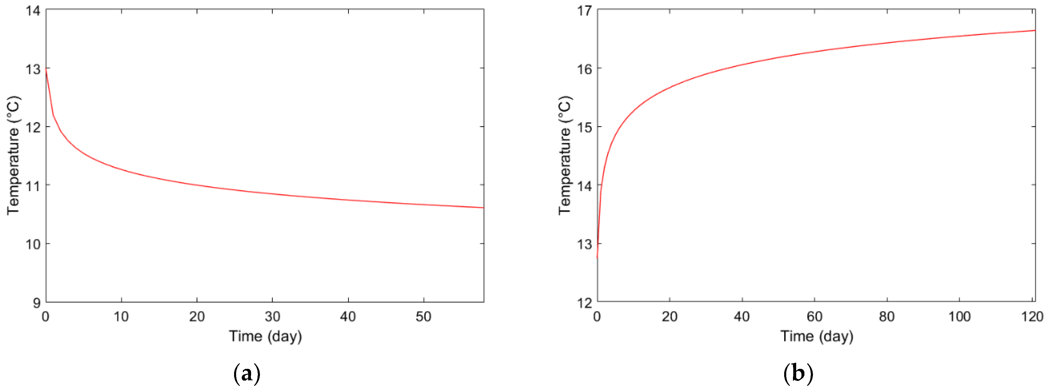
First, the results of ground temperature variation were investigated. It was observed that the ground temperature varies with distance from the center of the borehole. In previous design methods, the borehole wall temperature was generally used as a reference for estimating the heat extraction rate.
Figure 1 shows the variations in the borehole wall temperature at the end of the operating time of each day.
As shown in
Figure 1, the borehole wall temperature gradually declines during the heating season and increases during the cooling season. In both the seasons, the temperature changes rapidly in the early days of operation but stabilizes with continued operation. A logarithmic trend line was fitted to the results of
Figure 1 using an R2 value of 0.9992, which fits both the curves.
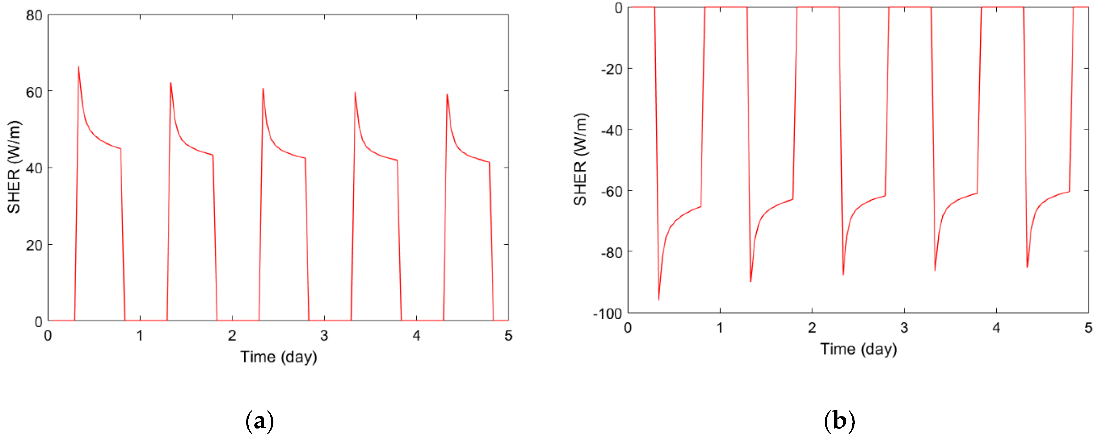
Additionally, the SHER was also investigated using the proposed model.
Figure 2 shows the variations in the SHER during the first five days of the heating and cooling seasons. The trend of SHER is logarithmic with an average R2 of 0.901 for the heating operation and 0.904 for the cooling operation. These results show that using a logarithmic trend line has the potential to estimate variations in SHER during operation.
3.3. Method for Estimating SHER
With the simulation results from the previous section, equations are derived to estimate the SHER and ground temperature. By expanding these results, sizing method for SHER can be established based on the following assumptions:
Only a single borehole of a single U-tube type was considered. The surrounding ground was assumed to be homogeneous and isotropic.
The ground had a uniform initial temperature. The heat loss or gain at the ground surface and effects of groundwater were neglected.
In extracting heating or cooling energy from the GHE, the entering temperature and mass flow rate of the circulating fluid were assumed to be constant.
As shown in
Figure 2, the value of SHER declines during the day and over a period of heating and cooling operations. This is due to a change in the ground temperature by an intermittent system operation. Nonetheless, the trend of daily change in SHER is almost the same over five days; however, the value of SHER differs every day. Thus, this study defined the general equation for estimating SHER during the operating time in a day as shown in Equation (1):
Equation (1) indicates that SHER can be estimated easily by solely inputting the time of a day. However, and pairs must be defined before they are used. Mathematically, and can be determined by using two different pairs of and . That is, if at two different time durations in a day are provided, it is possible to determine and . During the day, a number of different values of exist at a particular time. In this study, s at the beginning and ending time periods of the operation are used.
For this purpose, another equation is established to determine
.
is defined as the quantity of heat transferred per borehole length by the circulation of a fluid along the pipe. Thus,
is simply defined as shown in Equation (2) by multiplying thermal conductance between the fluid and surrounding material and the temperature difference between them. In Equation (2), arithmetic average of the inlet and outlet fluid temperatures are used.
The heat transfer between the fluid and surrounding material induces a change in the temperature of the fluid. In other words,
can also be defined as shown in Equation (3) based on the increase or decrease of fluid temperature.
Combining Equations (2) and (3), a new Equation (4) for the fluid outlet temperature is obtained as:
By substituting
into Equation (3), Equation (5) for SHER is obtained as:
In Equation (5), several parameters are required to calculate
with
being the most significant. According to
Figure 1, the ground temperature gradually increases or decreases in the cooling and heating seasons, respectively. Change in the ground temperature is greatly affected by the amount of heat transfer between the fluid and ground. Hence, the ground temperature in Equation (5) can be estimated by considering the amount of heat transfer. Nonetheless,
and
thermally depend on each other; hence, it is difficult to estimate
by considering the effect of each parameter. However,
can also be defined based on the results included in
Figure 1. The trend curve of ground temperature change is defined as a general equation based on Equation (3) as shown in Equation (6) that is given by:
By inputting the number of days in Equation (6), it is easy to obtain . In addition, the usage of and facilitates the estimation of considering the effect of amount of heat transfer. For example, the ground temperature changes rapidly when the amount of heat transfer is significant. Additionally, the change in ground temperature along the period is also significant. In this case, the value of determined will be large. Therefore, instead of inputting the amount of heat transfer directly in Equation (6), the values of and can be used to estimate the ground temperature considering its effect.
Similarly, and can also be determined. Two different pairs of and are used to determine and . In this study, the ground temperatures at the end of the first and second days are estimated, and then they are used as input for determining both the parameters. The ground temperature at the end of the day can be estimated by calculating the rise or drop in temperature by daily operation, which is a consequence of heat transfer between the fluid and surrounding material. Hence, Equation (1) can be used for calculating the amount of heat transfer for a day.
Besides the determination of parameters in Equations (1) and (6), estimation of the equivalent thermal conductance in Equation (5) is also significant. Since thermal conductance is the reciprocal of thermal resistance, this study focuses on finding a suitable method for determining thermal resistance based on the effect of heat transfer inside the borehole. This means that thermal interference between pipes must be considered along with convection inside the pipe and conduction between the fluid and surrounding material. Therefore, we have defined equivalent thermal conductance as shown in Equation (7) by referring to the concept of an effective borehole thermal resistance [
20].
4. Verification
Verification was performed to confirm that the sizing method can estimate the SHER accurately under different parameters including intermittent operating conditions. A total of 10 design cases were set up for the purpose of verification. For each design case, the SHER was calculated using the proposed design method and compared with the results obtained by transient simulation.
The two sets of results were examined by the coefficient of variation of the root mean square error (CV(RMSE)). CV(RMSE) is an index commonly used to calibrate building performance simulation models depicting the normalized measure of variability between measured and simulated values [
21,
22]. It is calculated using Equation (11) [
23].
where
According to the M&V guideline [
23], acceptable tolerance of CV(RMSE) is 15% at a monthly level and 30% at an hourly level.
4.1. Design Cases for Verification
The proposed design method is only capable of a single-borehole design using a single U-tube borehole type. Thus, verification was performed for a single borehole. Nonetheless, the number of design variables and performance parameters that influence the performance of GHE can be identified. Among them, the most influential design variables and performance parameters were selected and combined to generate the design conditions.
A previous study [
24] investigated the effects of major factors on the performance of the GCHP. Using these findings, the influential variables were chosen to be thermal conductivity and specific heat of the ground and grout material, length of the GHE, initial ground temperature, and fluid mass flow rate. In addition, intermittent operating conditions were applied.
It was observed that the values of the variables in design case 1 were the same as that of the simulation input values in the previous section. Based on design case 1, design cases 2 through 10 were generated by changing only one variable. The values of the influential variables for each of the design cases are described in
Table 2. The remaining design variables and performance parameters were constant for all the design cases. These values are listed in
Table 1.
4.2. Results of the Ground Region Temperature
Verification was performed by estimating the change in temperature of the ground and SHER. In the design method, the ground region temperature is calculated at an interval of a day; however, in the transient simulation, the temperatures of each node within the ground region are calculated at every time step of 6 min. The spatial average temperature was calculated for every node in the transient simulation and then compared with the results of the design method.
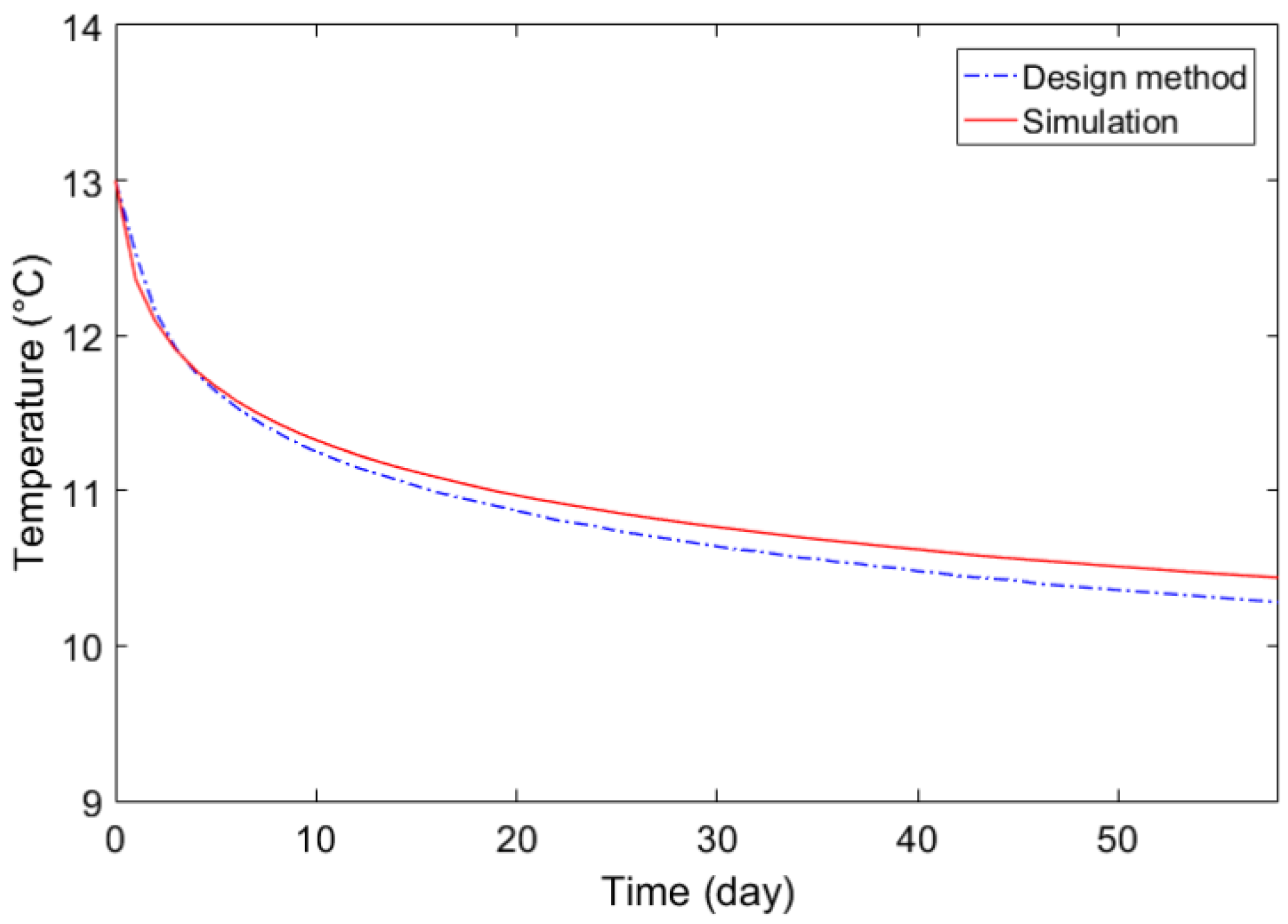
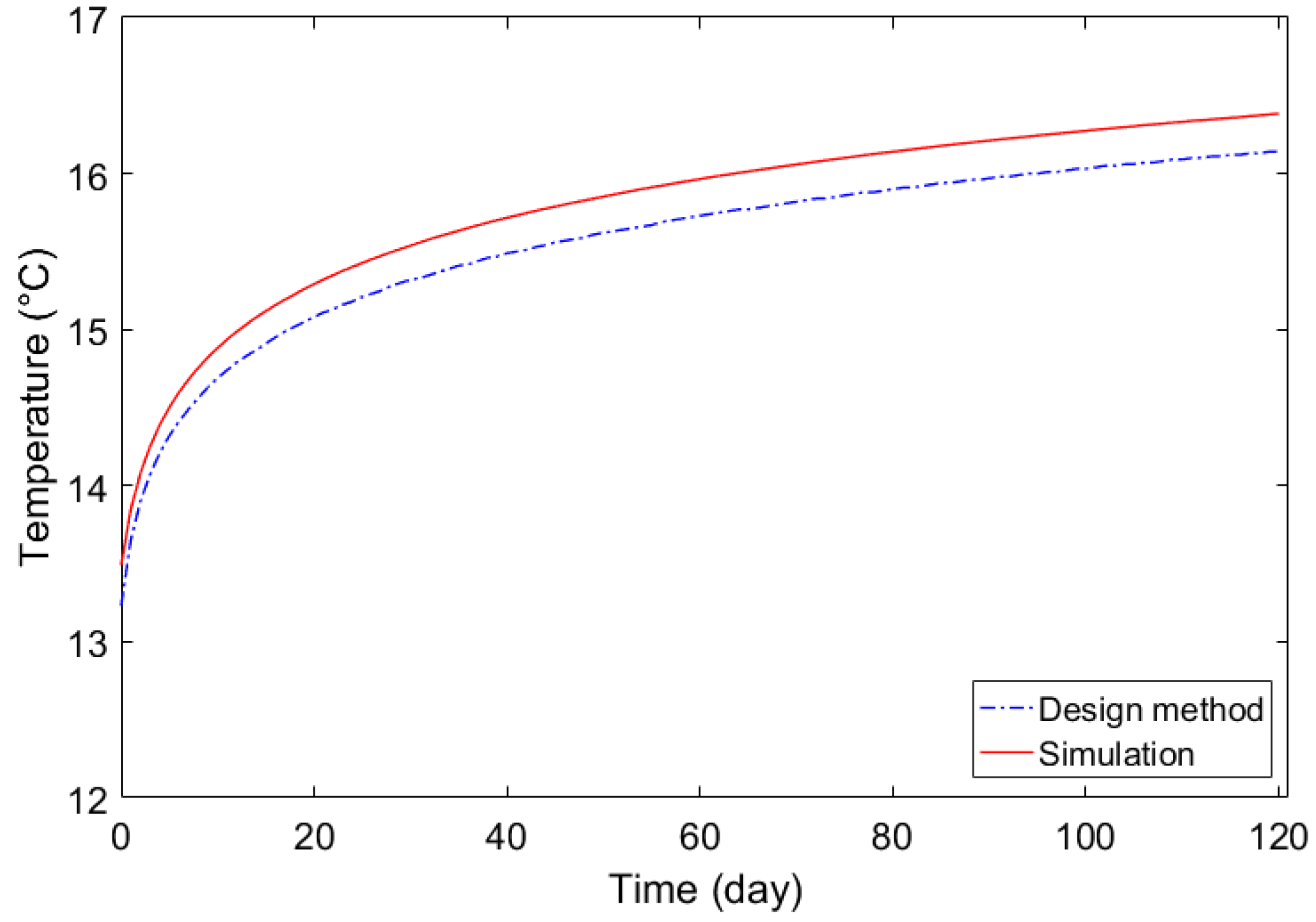
First, the ground region temperature change trends were compared.
Figure 3 and
Figure 4 show the change in the ground region temperature during the heating and cooling seasons of design case 1. For both the seasons, the ground region temperature changed rapidly in the early days of operation but slowed down in the latter days of operation. Overlaying the results, the curves of the ground region temperature change from both the design method and transient simulation appear similar.
Although the initial ground temperatures were the same, the temperature difference between the design method and transient simulation increased slightly as the heating and cooling operations continued. Consequently, by examining the temperature difference between the design method and transient simulation in a later operation period, we can assess whether using the design method is sufficient for designing GHEs. The ground region temperatures at the end of each season for both approaches are summarized in
Table 3. To determine the differences between the two approaches, the CV(RMSE) for each case is calculated.
Among the results of the ten design cases, the largest ground region temperature difference during the heating season was in case 4 at 0.76 °C. During the cooling seasons, the largest ground region temperature difference was in case 5 at 1.18 °C. Examining the CV(RMSE), the largest difference during the heating season was in case 4 at 5.28%. During the cooling season, the largest difference was 6.41% in case 5. All the values of CV(RMSE) in
Table 3 are smaller than 7% and are consistent with the design method and the transient simulation.
4.3. Results of SHER
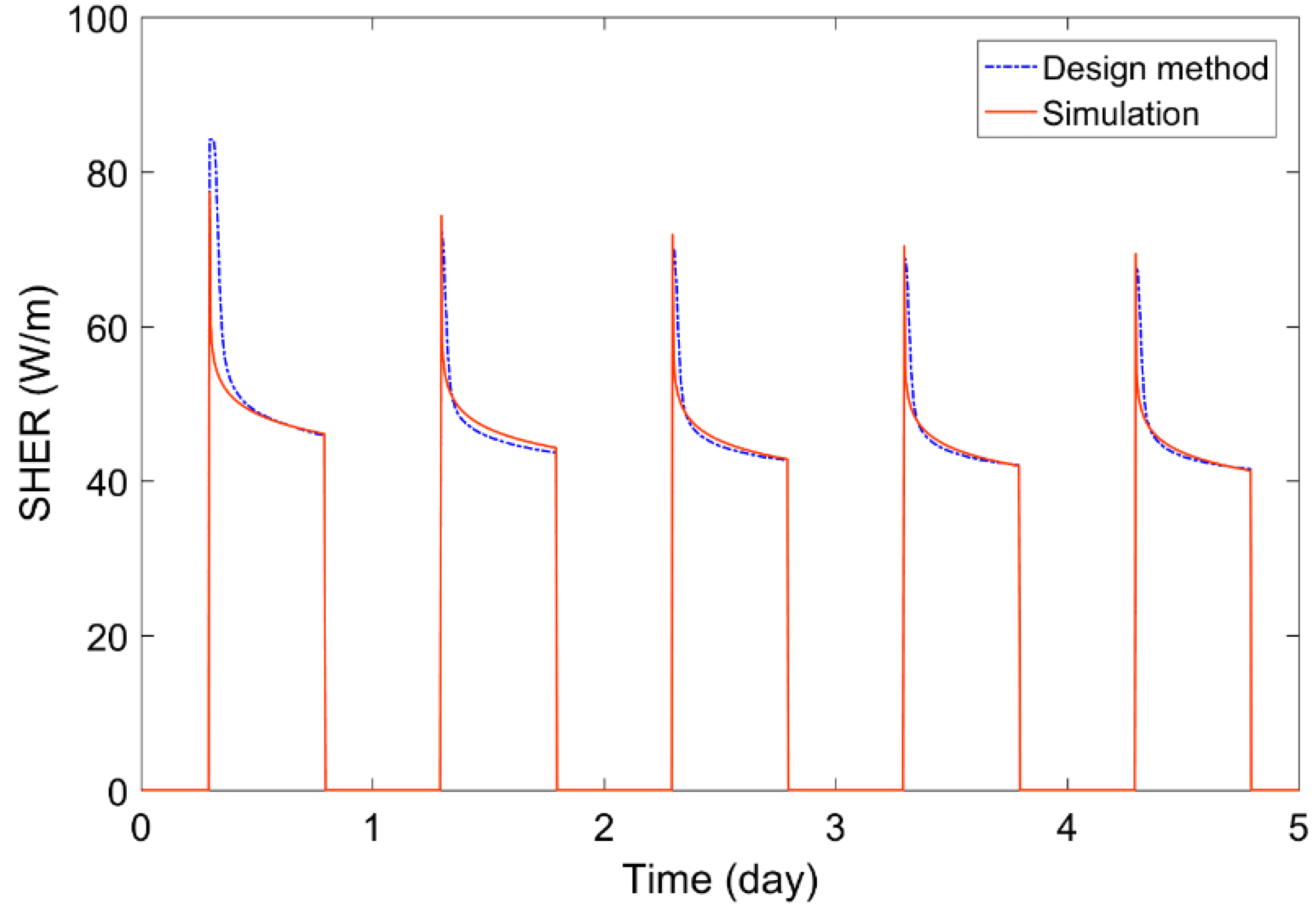
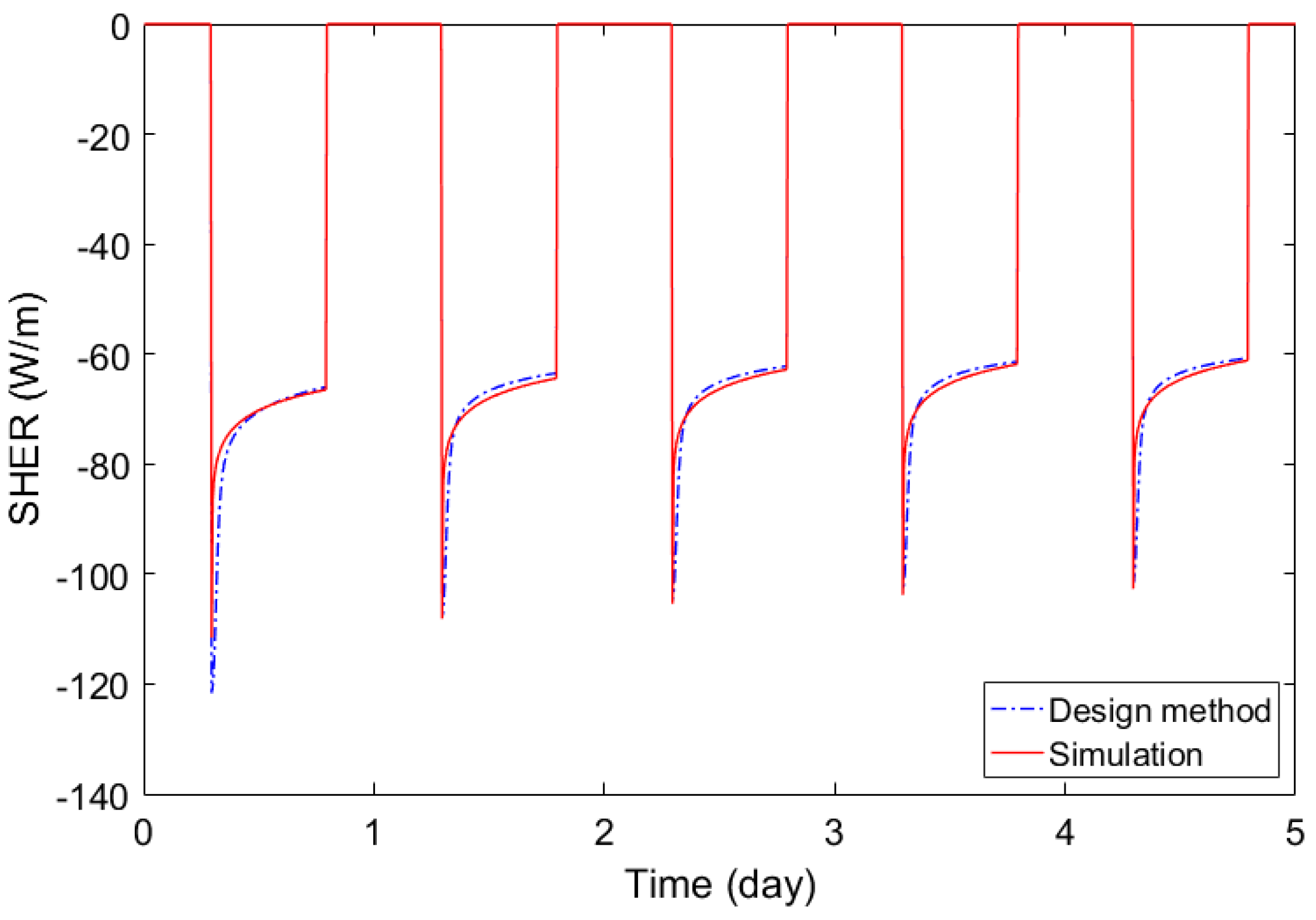
The second step of verification compares the change in SHER using the design method and transient simulation.
Figure 5 and
Figure 6 show the variations in SHER within the first five days of the heating and cooling seasons of design case 1. The SHER declines rapidly during the early minutes of the operating time; however, it declines gradually during the late hours. Similar to the results of the ground region temperature, the trends of change in SHER of the design method and the transient simulation are similar.
The SHER gradient for a day of the design method appears to be steeper than that of the transient simulation and in the early minutes of operation, both heating and cooling SHER of the design method are larger than those of the transient simulation. In the later hours of operation, both heating and cooling SHER of the design method are estimated to be smaller than those of the transient simulation. This means that the SHER of the design method was slightly overestimated for early operating minutes but underestimated for later operating hours.
To examine the estimated accuracy of the SHER, the CV(RMSE) was calculated for each case. Additionally, the average SHER for the heating and cooling seasons using both methods was calculated for comparison. The average SHER for the heating and cooling seasons and CV(RMSE) are listed in
Table 4.
For the ten design cases, the greatest difference between the average SHER of the heating season for the two methods was 2.45 W/m in case 3. For the cooling season, the largest difference was 2.85 W/m in case 10. Regarding the CV(RMSE), the largest difference for the heating season was 14.97% in case 7. The largest difference of CV(RMSE) for the cooling season was 12.44% in case 7. These results are also consistent with the design method and transient simulation.
4.4. Discussion on the Applicability of Design Method
According to these results, even if the ground region temperature and SHER were estimated using significantly approximated equations, the proposed design method would still produce a GHE with satisfactory performance. The practical applicability of the design method for designing GHEs under different design conditions was further investigated based on the results of verification.
The practical applicability of the design method for GHEs under different design conditions was further investigated based on the verification results. Firstly, the results of design cases 1 and 7 were compared to investigate the effects of a borehole size on the performance of GHE. The results showed that the average SHER for heating and cooling seasons increased from 22.5% to 24.1%, respectively. Even though SHER is expressed as heat transfer rate per length, the amount of heat extracted from the ground is higher for a longer borehole.
Other significant design parameters, thermal conductivities of a ground, and grouting material are also investigated to verify their effects on SHER of a GHE. According to the results of design cases 2, 1, and 3, the SHER for heating season increased by 28.5% and 41.5%. Similarly for cooling season, it increased from 30.8% to 41.6%. A similar tendency was observed in the cases based on the effects of thermal conductivity of the grout material. Comparing cases 4, 1, and 5, as the thermal conductivity of the grout changed by 0.68, 1.6, and 2.2 W/mK, respectively, the SHER increased from 17.4% to 26.4% during the heating season and from 18.4% to 28.3% during the cooling season. In the design of GHEs, the thermal conductivities of the ground and grout materials are the most significant performance parameters and these results verify their significant influence.
In addition, the effect of an initial ground temperature on SHER has been highlighted in this study. On comparing cases 1 and 8, the initial ground temperature increased from 13 to 15 °C, and the SHER increased by 19.4% during the heating season and decreased by 13.3% during the cooling season.
Lastly, comparing the results of case 1 with a 12 h operating time with those of case 9 with an 8 h operating time, the effects of heating and cooling operation time periods on SHER were investigated. The average SHER of the heating and cooling seasons increased by 5.7% and 3.0%, respectively. However, the comparison of case 1 with case 10 and a 16 h operating time revealed that the average SHER of the heating and cooling seasons decreased by 3.4% and 0.7%, respectively. The positive impact of increasing the stop time of the system has been proven in several studies. Hence, the results obtained in this study indicate that by increasing the stop time, SHER can be increased.
5. Conclusions
In this study, a novel sizing method was proposed for a single GHE. To consider the effects of heating and cooling operations of a building as well as those of soil properties, the estimate function for the SHER and ground region temperature was derived from the results of the transient simulation. For verification, ten design cases were generated by combining different values of influential performance parameters. This study identified that the CV(RMSE) for all ten design cases was lower than 15% during the heating and cooling seasons. Based on the results and criteria suggested by the standard, it was concluded that the proposed design method was capable of designing a GHE under different influential variables and intermittent operating conditions.
The influential parameters considered for the proposed method were initial ground temperature, building heating and cooling operation, and soil thermal properties. These parameters were determined in the early design stage. Hence, the proposed method was used in the early design stage to estimate the SHER. Moreover, the methods consisted of simple equations that help the architects to estimate SHER by simply inputting values into equations.
However, this method has limitations. The applicability of the proposed method is limited to a single borehole with a single U-tube type. Because multiple boreholes are commonly adopted in buildings, further research is essential to expand the applicability of the proposed design method.


