Laboratory Measurement and Boundary Conditions for the Water Vapour Resistivity Properties of Typical Australian Impermeable and Smart Pliable Membranes

Abstract

The duo of better insulated and more air-tight envelopes without appropriate consideration of water vapour diffusion and envelope moisture management has often demonstrated an increased potential of moisture accumulation, interstitial condensation, and mould growth within the building envelope. To inform a resilient, energy efficient, and healthy building design, long-term transient hygrothermal modelling are required. Since 2008, concern has been raised to the Australian building regulators regarding the need to establish the vapour diffusion properties of construction materials, in order to develop a hygrothermal regulatory framework. This paper discusses the results from laboratory testing of the vapour diffusion properties of two common reflective pliable membranes, and one smart pliable membrane. The two reflective pliable membranes are often used within the exterior walls of Australian buildings. The smart pliable membrane is a relatively new, internationally available product. The three membranes were tested as per ISO 12,572 at 23 °C and 50% RH. To establish if the vapour resistivity properties were constant, under different relative humidity conditions, the membranes were further tested at 23 °C and relative humidity values of 35%, 65%, and 80%. The results of the three pliable membranes show that the vapour resistivity properties varied in a non-linear (dynamic) manner subject to relative humidity. In conclusion, this research demonstrates that regardless of the class, each of the tested membrane types behaved differently under varying relative humidity and pressure gradients within the testing laboratory.

1. Introduction

The aim of this research was to investigate whether the single point vapour resistivity test method as described in ISO 12572 and ASTM E 96m provides adequate data to inform building envelope hygrothermal simulation. The current standard only requires a single point measurement for materials tested at 23 °C and 50% relative humidity (RH). The incorporation of high-quality material property inputs in the hygrothermal simulation has been identified by many as critical, which may significantly impact the moisture and mould risk calculations. This article reports on the observed water vapour resistivity properties of two impermeable pliable membranes, and one smart pliable membrane, when tested under different relative humidity conditions (humidity-dependent), in order to plot multiple point, rather than single point, hygrothermal boundary curves for each of these materials.

The combination of thermal insulation and airtightness without appropriate consideration of the external envelope’s ability to manage water vapour diffusion and moisture have been identified as key contributors to moisture, moisture accumulation, and mould growth within internal and interstitial spaces in energy efficient buildings [1,2,3,4]. Since the 1990s, design processes have increasingly included complex hygrothermal simulation methods, which calculate moisture accumulation and mould growth. In 2019, Australia’s national building regulations, the National Construction Code (NCC), included the first performance requirement regarding condensation. These regulations were the result of significant market-based concerns about the visible presence of condensation and mould prevalent in many Australian new buildings. The performance requirement states, “Risks associated with water vapour and condensation must be managed to minimise their impact on the health of occupants” [5]. Reflecting the universal acceptance that mould spores affect human health, the new clauses were included within the Health and Amenity section [6,7,8]. In Australia, the development of guidelines, policy, and the regulatory framework regarding material data and bio-hygrothermal simulation methods is of importance due to the increased requirements for highly energy-efficient buildings and the corresponding development of condensation-related regulations for 2019, 2022, and 2025.

In this research, the water vapour resistivity properties of two types of impermeable membrane, and one type of smart pliable membrane were measured under different relative humidity conditions. Following international methods, the data was then modified to obtain variable hygrothermal boundary curves for inclusion in hygrothermal simulation. The effect of the differences between hygrothermal simulations completed using a single point, or a multi-point hygrothermal boundary curve will be reported in a future article. Within this context, the research collaboration between the University of Tasmania and Fraunhofer Institute of Building Physics (IBP) Germany, also addressed the matter of how to establish the hygrothermal boundary curves for materials tested via the gravimetric cup method and under different relative humidity conditions. This boundary curve is of great importance, especially if it is identified that construction materials have variable characteristics subject to different relative humidity conditions [9,10,11]. This is because the vapour resistivity properties of construction materials is not constant across the boundary curve but varies continuously along the cross-section of such materials. Previous publications about this research project have described the advanced method for construction material water vapour resistivity testing that has been completed to assist in providing high quality data for hygrothermal simulation.

There has been a growing concern that the standard testing method normally adopted in North America and Europe may provide insufficient hygrothermal guidance for the design guidance of building envelopes [2,12,13,14,15]. The current methods were developed at a time of limited computer processing capacity and for non-transient simulation methods. This method has been critiqued internationally, due to its focus on a single environmental condition, namely, 23 °C and 50% RH, which may not adequately represent the conditions within the external envelope [2,13,16]. Currently, Australia has adopted the North American Testing Method, ASTM E 96m, to obtain water vapour diffusion properties, as referenced in Australia Standard, AS4200:1, which deals with the application of pliable membranes in buildings [17,18]. As Australia seeks a more detailed climatically- based approach to address surface and interstitial moisture problems in buildings, it has been acknowledged that there is a need to quantify construction material’s hygrothermal diffusion characteristics under different relative humidity conditions that may better represent the boundary conditions within external walls [13]. Relative humidity considerations are important, as the normal level of relative humidity varies significantly between climate types, whether they be desert, cool/temperate, maritime, or hot and humid climates. ASHRAE Standard 160 recommends interior relative humidity (RH) conditions be maintained between 30 and 60% [19]. Several researchers have identified internal relative humidity levels within occupied, conditioned, and unconditioned housing well above the 50% RH level prescribed in the single point vapour resistivity test method [16]. To adequately complete hygrothermal simulations requires appropriately detailed interior and exterior climatic data and precise water vapour diffusion properties for each material in the external envelope. A common standpoint for any simulation-based decision making is: garbage in—garbage out. Similarly, as buildings become more complex, apply increased air tightness and insulation levels, increase the use of sustainable/renewable construction materials, and include many materials within an envelope system, the sensitivity of the hygrothermal model to any change may significantly impact on the simulation result [20]. To enhance and give confidence to the accuracy of hygrothermal simulations, which predict the wetting, drying, and mould growth potential, a more comprehensive understanding of the vapour resistivity properties of all materials used in the external envelope of buildings is required under different temperate and relative humidity conditions.

The application of pliable membranes has a long history and is common in many sectors. Increasingly, the advancement of pliable membranes will continue to usher new opportunities within the construction sector [21,22,23]. However, in the building design and construction industry, pliable membranes used to assist building energy efficiency have gone through many stages of product development, and manufacturers have used many terminologies to drive the marketing values of different products. These terms include vapour retarder, thermal barrier, vapour barrier, water resistive barrier, air barrier, damp proof membrane, weather barrier, and breathable building wrap. In Australia, these terms are often misunderstood and confused when considering the selection for building design and construction. The most acceptable way to define and classify different types of pliable membranes is according to their degree of resistance to gas or vapour transport, which is either permeable, semi permeable, semi-impermeable, and impermeable [13,21]. Furthermore, climate change is driving national demand for more airtight and energy-efficient buildings, progressively requiring manufacturers to create more innovative products. This is expected to allow new buildings to be more resilient, supportive, and responsive to changing interior and exterior climates, and improve the building envelope thermal performance and indoor air quality. Depending on the polymer, or other technology, of these products, manufacturers are now shifting towards the use of the terms such as smart or variable vapour diffusion/resistivity membranes to describe these new generations of product lines. An impermeable membrane is usually referred to as a vapour barrier because they do not allow water vapour diffusion to occur through the membrane. On the other hand, semi-impermeable membranes do allow moderate vapour diffusion through the membrane. However, their vapour resistance factor and air layer equivalent thickness values are moderate, but still high in comparison to a permeable membrane, which is very open to the vapour diffusion process [24].

Previously, this research program has measured and reported the vapour diffusion properties of other types of pliable building membranes. Like the research reported in this article, the water vapour diffusion properties were measured under different relative humidity conditions. This research revealed that vapour permeable pliable membranes which were identified as Class 3 and Class 4, within the Australian Standards (AS4200), behaved differently and in a non-linear manner under different relative humidity conditions [13].

Therefore, this paper reports on the results obtained from laboratory gravimetric cup measurements and the method employed to plot the hygrothermal boundary curves of two types of vapour impermeable, and reflective, pliable membranes, and one type of semi-impermeable (commonly called variable) pliable membrane. The reflective and vapour impermeable pliable membrane products are often used within the exterior timber and steel-framed walls of Australian buildings, and classified as a class 1 vapour control membrane (0.0 to 0.0022 μg/N/s) in AS4200 [17]. Similarly, the smart pliable membrane is a relatively new, internationally available product and is classified as a class 2 vapour control membrane (0.022 to 0.1429 μg/N/s) in AS4200:1.

2. Materials and Methods

The methodology involved undertaking gravimetric testing of the water vapour resistivity characteristics of two types of impermeable membranes and one type of smart membrane in a laboratory environment. For easy identification purposes in this paper, the sample from the smart membrane is tagged as specimen C, while samples from the two impermeable reflective pliable membranes are tagged specimen D and E, respectively. These membranes are commonly applied to the external face of the timber or steel frame (outside the insulation layer), of low-rise buildings, to improve air tightness (thermal performance), as a water barrier (façade durability), and as a vapour control layer (condensation and mould) in walls and roofs of buildings. The two types of impermeable membrane were reflective foil products from different manufacturers. They both had similar polymer characteristics and were coated with aluminium foil on the surface of one side. The smart membrane, which is commonly used in walls and roofs is a polyethylene copolymer product with varying water vapour diffusion properties, subject to the air moisture content. The total measurement period for all pliable membrane testing took fourteen months, which involved four experiments during which the temperature was maintained at 23 °C and the relative humidity conditions of the hygrothermally-controlled room were maintained at 35%, 50%, 65%, and 80%, respectively. Since the three membrane types discussed here are not readily open to the water vapour diffusion process, it took an average of three and a half months to establish a moisture equilibrium state for each specimen for each period of relative humidity conditioning.

2.1. Boundary Conditions

The experiments are based on the principle of diffusion of water vapour from an area with higher partial pressure of water vapour to an area with lower partial pressure. In these experiments, the vapour drive was established as a result of the pressure differences between the relative humidity within the internal air space of the test dish and the relative humidity within the internal condition of the hygrothermal testing room. This creates partial vapour pressure differences which cause water vapour diffusion to occur, which is similar to what the external building envelope may be experiencing in real life. The production and control of the testing room for these experiments has been discussed in previous publications. To avoid both air temperature and humidity stratification within the test room, a fan was in operation throughout the entire measurement period. This fan generated an air velocity of approximately 0.2 m/s which stabilised the pressure within the room. The average air temperature of the room was maintained at 23 °C throughout the four periods of measurement with ±1 °C variation. The relative humidity and their vapour pressure differences, which represent the targeted boundary condition for the four periods of the experiment, are shown in

Table 1. ΔP values for each of the test conditions.

Experimental Period	Temperature (°C)	Relative Humidity (Dry Side) (%)	Relative Humidity (Wet Side) (%)	Water Vapour Pressure Difference ΔP (Pa)
1 dry test	23	3	35	898
1 wet test	23	35	93	1628
2 dry test	23	3	50	1319.8
2 wet test	23	50	93	1207.25
3 dry test	23	3	65	1740.74
3 wet test	23	65	93	786.12
4 dry test	23	3	80	2161.83
4 wet test	23	80	93	364.99

. This table was adapted from ISO 12,572 with additional testing points that were identified based on common climatic condition adopted for the four testing periods in this research. This table is important as it provides input data for the calculation and tabulation of the vapour resistivity properties of materials involving multiple moisture-dependent variables, which are needed to plot the hygrothermal curves that reflect different boundary conditions. In each of the experiments, the relative humidity in the hygrothermally-controlled room was carefully controlled. The relative humidity was maintained between 35.0% to 36.9%, with an average of 36% in the first test period. In the second test period, the relative humidity was maintained between 49.8% to 50.8%, with the average humidity of 50.4%. The relative humidity was maintained between 64.5% to 65.2%, with an average relative humidity of 65.12% in the third test period. During the fourth test period, the relative humidity was maintained between 77.84% to 83.2% with an average relative humidity of 80.29%. The details about the temperature and relative humidity performance of the chamber with respective variation has been reported in the previous publication [13].

2.2. Experimenal Procedure

The gravimetric procedure employed in this research followed the guidelines of the international standard ISO 12,572 [25]. The procedure involved completing both wet cup and dry cup gravimetric water vapour transmission measurement for samples from the three membranes. In each testing period, ten specimens were cut from the smart membrane (C), and another ten specimens from each of the two types of impermeable membrane (D). For each of the pliable membranes, five of these specimens were for wet cup testing and five specimens were for dry cup testing. Due to the amount of sample material provided, only six specimens were prepared for the second type of impermeable membrane (E), representing three specimens for wet cup and three specimens for the dry cup test. The test dishes comprised a round glass dish with 200 mm diameter and a 60 mm depth. The thickness of each specimen was measured by a digital micrometre screw gauge over ten different points on the surface of each specimen and the mean value was determined and recorded for later use during the water vapour diffusion calculation process. The specimens were precisely cut to the dish size (200 mm) such that they fit to the edge of the mouth of the dishes. The desired relative humidity within the cups were achieved by the use of dry and wet substrates. This research adopted silica gel as dry cup substrate because it was very stable at 3% relative humidity. The wet cup test achieved the desired relative humidity of 93% through the use of anhydrous ammonium dihydrogen phosphate solution at 23 °C. The substrates were gently poured into the dishes until an airspace of 20 mm was established between the top of the substrate and the top of the test dish. The specimens were then sealed to the edge of the test dishes with glue, followed by tightly wrapping the edge of the dishes with paper tape. To achieve adequate vapour seal, paraffin wax of 6:4 ratio and melting at 58–60 °C was gently applied around the paper tape with an artist’s brush until the paper tape was no longer visible and the molten wax was allowed to harden. The gravimetric measurement began once a set of five specimens were completed for a particular test. Given that the temperatures inside the cup and outside the cup are the same, partial vapour pressure differential was achieved by the difference between the conditioned room’s relative humidity and the wet or dry substrate within each dish, causing water vapour diffusion through the test specimen. The amount of water vapour diffusion was established by periodically measuring the weight of the cup assembly. The measurement of the dish weight continued until a steady state was reached. However, due to these membranes being vapour impermeable, after an initial period of regular measurements, the time between measurements was expanded to once a week, for a period of three months, and the diffusion properties of the specimens were determined through mathematical calculations.

3. Results

The result for the water vapour resistivity properties for each specimen tested was calculated from the mathematical equations provided by the ISO 12,572 [25]. The mathematical calculation and procedure for obtaining various iterative resistivity properties using specimen C 1 as an example is presented in the Appendix A. This calculation procedure was repeated for all the specimens, for all the boundary conditions (35%, 50%, 65%, and 80%). The detail results for the properties of each membrane tested and the statistical analysis for all the four testing periods are tabulated in Appendix C 

Table A2. Water vapour resistivity properties for sample C at 35% RH 23 °C.

Sample	Mean Thickness	Mass Change Rate	Area	Water Vapour Flux	Water Vapour Permeance	Water Vapour Resistance	Water Vapour Permeability	Water Vapour Resistance	Diffusion-Equivalent
at 23 °C 35% RH	d (m)	/time (G in kg/s)	m2	g = G/A in kg/(s·m2)	W = g/dp in kg/(s·m2·Pa)	Z = 1/W in (s·m2·Pa)/kg	δ = W × d in kg/(s·m·Pa)	factor µ	air layer thickness Sd
Dry cup test
C-1	0.000213	1.2 × 10−10	0.02830	4.3 × 10−9	4.7 × 10−12	2.1 × 1011	1.0 × 10−15	193,866.0000	41.2900
C-2	0.000248	9.8 × 10−11	0.02630	3.7 × 10−9	4.2 × 10−12	2.4 × 1011	1.0 × 10−15	189,233.8700	46.9300
C-3	0.000256	9.2 × 10−11	0.02540	3.6 × 10−9	4.0 × 10−12	2.5 × 1011	1.0 × 10−15	188,509.8800	48.2600
C-4	0.000256	9.8 × 10−11	0.02750	3.6 × 10−9	4.0 × 10−12	2.5 × 1011	1.0 × 10−15	191,794.3500	49.1000
C-5	0.000252	9.8 × 10−11	0.02600	3.8 × 10−9	4.2 × 10−12	2.3 × 1011	1.1 × 10−15	183,888.8900	46.3600
Mean	0.000245	1.0 × 10−10	0.02670	3.8 × 10−9	4.2 × 10−12	2.4 × 1011	1.0 × 10−15	189,458.5980	46.3880
Wet cup test
C-6	0.000246	2.8 × 10−9	0.02630	1.1 × 10−7	6.6 × 10−11	1.5 × 1010	1.6 × 10−14	11,910.5800	2.9300
C-7	0.000287	2.3 × 10−9	0.02780	8.2 × 10−8	5.0 × 10−11	2.0 × 1010	1.4 × 10−14	13,491.7600	3.8700
C-8	0.000255	2.2 × 10−9	0.02690	8.2 × 10−8	5.1 × 10−11	2.0 × 1010	1.3 × 10−14	15,034.3300	3.8340
C-9	0.000251	2.6 × 10−9	0.02690	9.6 × 10−8	5.9 × 10−11	1.7 × 1010	1.5 × 10−14	13,149.6300	3.3000
C-10	0.000253	2.9 × 10−9	0.02780	1.0 × 10−7	6.3 × 10−11	1.6 × 1010	1.6 × 10−14	12,090.9500	3.0600
Mean	0.0002584	2.6 × 10−9	0.02714	9.4 × 10−8	5.8 × 10−11	1.8 × 1010	1.5 × 10−14	13,135.4500	3.3988

,

Table A3. Water vapour resistivity properties of sample C at 23 °C 50% RH.

Sample Tested	Mean Thickness	Mass Change Rate	Area	Water Vapour Flux	Water Vapour Permeance	Water Vapour Resistance	Water Vapour Permeability	Water Vapour Resistance	Diffusion-Equivalent
at 23 °C 50% RH	d (m)	/time (G in kg/s)	m2	g = G/A in kg/(s·m2)	W = g/dp in kg/(s·m2·Pa)	Z = 1/W in (s·m2·Pa)/kg	δ = W × d in kg/(s·m·Pa)	factor µ	air layer thickness Sd
Dry cup test
C-1	0.000213	3.2 × 10−10	0.02830	1.1 × 10−8	8.6 × 10−12	1.2 × 1011	1.8 × 10−15	106,291.0800	22.6600
C-2	0.000248	2.4 × 10−10	0.02630	9.3 × 10−9	7.0 × 10−12	1.4 × 1011	1.7 × 10−15	111,688.4600	27.7000
C-3	0.000256	2.9 × 10−10	0.02550	1.2 × 10−8	8.8 × 10−12	1.1 × 1011	2.2 × 10−15	86,641.7800	22.1800
C-4	0.000256	3.2 × 10−10	0.02750	1.2 × 10−8	8.8 × 10−12	1.1 × 1011	2.3 × 10−15	85,962.4200	22.0100
C-5	0.000252	3.0 × 10−10	0.02600	1.1 × 10−8	8.6 × 10−12	1.2 × 1011	2.2 × 10−15	89,654.7600	22.5900
Mean	0.000245	2.9 × 10−10	0.02672	1.1 × 10−8	8.4 × 10−12	1.2 × 1011	2.0 × 10−15	96,047.7000	23.4280
Wet cup test
C-6	0.000246	2.9 × 10−9	0.02630	1.1 × 10−7	9.1 × 10−11	1.1 × 1010	2.2 × 10−14	8570.3800	2.1100
C-7	0.000287	2.6 × 10−9	0.02780	9.2 × 10−8	7.6 × 10−11	1.3 × 1010	2.2 × 10−14	8810.0270	2.5300
C-8	0.000251	3.8 × 10−9	0.02690	1.4 × 10−7	1.2 × 10−10	8.5 × 109	3.0 × 10−14	6494.0200	1.6300
C-9	0.000251	3.9 × 10−9	0.02550	1.5 × 10−7	1.3 × 10−10	8.0 × 109	3.2 × 10−14	6091.5500	1.5300
C-10	0.000253	3.8 × 10−9	0.02780	1.4 × 10−7	1.1 × 10−10	8.9 × 109	2.8 × 10−14	6758.0000	1.7100
Mean	0.0002576	3.4 × 10−9	0.02686	1.3 × 10−7	1.0 × 10−10	9.9 × 109	2.7 × 10−14	7344.7954	1.9020

,

Table A4. Water vapour resistivity properties of sample C at 23 °C 65% RH.

Sample Tested	Mean Thickness	Mass Change Rate	Area	Water Vapour Flux	Water Vapour Permeance	Water Vapour Resistance	Water Vapour Permeability	Water Vapour Resistance	Diffusion-Equivalent
at 23 °C 65% RH	d (m)	/time (G in kg/s)	m2	g = G/A in kg/(s·m2)	W = g/dp in kg/(s·m2·Pa)	Z = 1/W in (s·m2·Pa)/kg	δ = W × d in kg/(s·m·Pa)	factor µ	air layer thickness Sd
Dry cup test
C-1	0.000229	5.6 × 10−10	0.02720	2.1 × 10−8	1.2 × 10−11	8.5 × 1010	2.7 × 10−15	72,237.3900	16.5400
C-2	0.000248	5.9 × 10−10	0.02750	2.1 × 10−8	1.2 × 10−11	8.2 × 1010	3.0 × 10−15	64,399.4000	15.9700
C-3	0.000256	6.1 × 10−10	0.02690	2.3 × 10−8	1.3 × 10−11	7.7 × 1010	3.3 × 10−15	59,677.9700	15.2800
C-4	0.000258	5.8 × 10−10	0.02750	2.1 × 10−8	1.2 × 10−11	8.3 × 1010	3.1 × 10−15	63,056.0000	16.2700
C-5	0.000252	5.6 × 10−10	0.02689	2.1 × 10−8	1.2 × 10−11	8.3 × 1010	3.0 × 10−15	64,375.2400	16.2200
Mean	0.0002486	5.8 × 10−10	0.02720	2.1 × 10−8	1.2 × 10−11	8.2 × 1010	3.0 × 10−15	64,749.2000	16.0560
Wet cup test
C-6	0.000277	1.9 × 10−9	0.02750	6.8 × 10−8	8.6 × 10−11	1.2 × 1010	2.4 × 10−14	8158.8500	2.2600
C-7	0.000284	1.7 × 10−9	0.02750	6.1 × 10−8	7.8 × 10−11	1.3 × 1010	2.2 × 10−14	8802.8200	2.5000
C-8	0.000278	2.0 × 10−9	0.02720	7.2 × 10−8	9.1 × 10−11	1.1 × 1010	2.5 × 10−14	7645.3800	2.1300
C-9	0.000262	1.7 × 10−9	0.02660	6.2 × 10−8	7.9 × 10−11	1.3 × 1010	2.1 × 10−14	9395.5200	2.4600
C-10	0.000263	1.6 × 10−9	0.02660	5.9 × 10−8	7.5 × 10−11	1.3 × 1010	2.0 × 10−14	9809.4800	2.5800
Mean	0.0002728	1.7 × 10−9	0.02708	6.4 × 10−8	8.2 × 10−11	1.2 × 1010	2.2 × 10−14	8762.4100	2.3860

,

Table A5. Water vapour resistivity properties of sample C at 23 °C 80% RH.

Sample Tested at 23 °C 80% RH	Mean Thickness d (m)	Mass Change Rate/Time (G in kg/s)	Area m2	Water Vapour Flux g = G/A in kg/(s·m2)	Water Vapour Permeance W = g/dp in kg/(s·m2·Pa)	Water Vapour Resistance Z = 1/W in (s·m2·Pa)/kg	Water Vapour Permeability δ = W × d in kg/(s·m·Pa)	Water Vapour Resistance Factor µ	Diffusion Equivalent Air Layer Thickness Sd
Dry cup test
C-1	0.000284	4.2 × 10−9	0.02720	1.5 × 10−7	7.1 × 10−11	1.4 × 1010	2.0 × 10−14	9628.2300	2.7300
C-2	0.000277	4.3 × 10−9	0.02750	1.5 × 10−7	7.2 × 10−11	1.4 × 1010	2.0 × 10−14	9797.8500	2.7100
C-3	0.000278	4.1 × 10−9	0.02690	1.5 × 10−7	7.0 × 10−11	1.4 × 1010	1.9 × 10−14	10,035.9700	2.7900
C-4	0.000262	4.2 × 10−9	0.02750	1.5 × 10−7	7.0 × 10−11	1.4 × 1010	1.8 × 10−14	10,584.5300	2.7700
C-5	0.000263	4.3 × 10−9	0.02690	1.6 × 10−7	7.4 × 10−11	1.4 × 1010	1.9 × 10−14	10,030.1700	2.6400
Mean	0.0002728	4.2 × 10−9	0.02720	1.5 × 10−7	7.1 × 10−11	1.4 × 1010	1.9 × 10−14	10,015.3500	2.7280
Wet cup test
C-6	0.000277	9.3 × 10−10	0.02750	3.4 × 10−8	9.2 × 10−11	1.1 × 1010	2.6 × 10−14	7476.8900	2.0700
C-7	0.000284	1.1 × 10−9	0.02750	4.1 × 10−8	1.1 × 10−10	8.9 × 109	3.2 × 10−14	5954.2400	1.6900
C-8	0.000278	1.2 × 10−9	0.02720	4.3 × 10−8	1.2 × 10−10	8.6 × 109	3.2 × 10−14	5882.1300	1.6400
C-9	0.000262	9.3 × 10−10	0.02660	3.5 × 10−8	9.5 × 10−11	1.0 × 1010	2.5 × 10−14	7643.6600	2.0000
C-10	0.000263	8.5 × 10−10	0.02660	3.2 × 10−8	8.7 × 10−11	1.1 × 1010	2.3 × 10−14	8314.1600	2.9000
Mean	0.0002728	1.0 × 10−9	0.02708	3.7 × 10−8	1.0 × 10−10	1.0 × 1010	2.8 × 10−14	7054.2160	2.0600

,

Table A6. Water vapour resistivity properties for sample D at 23 °C 35% RH.

Sample Tested at 23 °C 35% RH	Mean Thickness d (m)	Mass Change Rate/Time (G in kg/s)	Area m2	Water Vapour Flux g = G/A in kg/(s·m2)	Water Vapour Permeance W = g/dp in kg/(s·m2·Pa)	Water Vapour Resistance Z = 1/W in (s·m2·Pa)/kg	Water Vapour Permeability δ = W × d in kg/(s·m·Pa)	Water Vapour Resistance Factor µ	Diffusion-Air Layer Thickness Sd
Dry cup test
D-1	0.000224	7.23 × 10−11	2.60 × 10−2	2.78 × 10−9	3.10 × 10−12	3.23 × 1011	6.94 × 10−16	281,432.34	63.04
D-2	0.00022	9.65 × 10−11	2.57 × 10−2	3.75 × 10−9	4.18 × 10−12	2.39 × 1011	9.19 × 10−16	212,427.32	46.73
D-3	0.000221	8.20 × 10−11	2.49 × 10−2	3.29 × 10−9	3.66 × 10−12	2.73 × 1011	8.10 × 10−16	241,020.61	53.27
D-4	0.000227	1.01 × 10−10	2.32 × 10−2	4.37 × 10−9	4.86 × 10−12	2.06 × 1011	1.10 × 10−15	176,990.51	40.18
D-5	0.000221	8.20 × 10−11	2.32 × 10−2	3.53 × 10−9	3.93 × 10−12	2.54 × 1011	8.69 × 10−16	224,580.78	49.63
Mean	0.000223	8.68 × 10−11	0.0246	3.54 × 10−9	3.95 × 10−12	2.59 × 1011	8.79 × 10−16	2.27 × 105	50.57
Wet cup test
D-6	0.00022	3.71 × 10−10	0.0275	1.35 × 10−8	8.24 × 10−12	1.21 × 1011	1.81 × 10−15	1.08 × 105	23.69
D-7	0.00022	3.08 × 10−10	0.0269	1.14 × 10−8	6.98 × 10−12	1.43 × 1011	1.54 × 10−15	1.27 × 105	27.96
D-8	0.00023	2.86 × 10−10	0.0263	1.09 × 10−8	6.64 × 10−12	1.51 × 1011	1.50 × 10−15	1.31 × 105	29.38
D-9	0.00022	2.97 × 10−10	0.0255	1.16 × 10−8	7.11 × 10−12	1.41 × 1011	1.57 × 10−15	1.24 × 105	27.46
D-10	0.00022	3.29 × 10−10	0.0263	1.25 × 10−8	7.63 × 10−12	1.31 × 1011	1.69 × 10−15	1.15 × 105	25.59
Mean	0.00022	3.18 × 10−10	0.0265	1.20 × 10−8	7.32 × 10−12	1.37 × 1011	1.62 × 10−15	1.21 × 105	26.816

,

Table A7. Water vapour resistivity properties for sample D at 23 °C 50% RH.

Sample Tested at 23 °C 50% RH	Mean Thickness d (m)	Mass Change Rate/Time (G in kg/s)	Area m2	Water Vapour Flux g = G/A in kg/(s·m2)	Water Vapour Permeance W = g/dp in kg/(s·m2·Pa)	Water Vapour Resistance Z = 1/W in (s·m2·Pa)/kg	Water Vapour Permeability δ = W × d in kg/(s·m·Pa)	Water Vapour Resistance Factor µ	Diffusion-Air Layer Thickness Sd
Dry cup test
D-1	0.000230	2.02 × 10−10	0.02750	7.33 × 10−9	5.56 × 10−12	1.80 × 1011	1.28 × 10−15	151,165	34.77
D-2	0.000223	3.17 × 10−10	0.02776	1.14 × 10−8	8.65 × 10−12	1.16 × 1011	1.93 × 10−15	100,117.68	22.33
D-3	0.000228	2.59 × 10−10	0.02750	9.43 × 10−9	7.14 × 10−12	1.40 × 1011	1.63 × 10−15	118,581.32	27.04
D-4	0.000227	2.02 × 10−10	0.02750	7.33 × 10−9	5.56 × 10−12	1.80 × 1011	1.26 × 10−15	153,171.81	34.77
D-5	0.000221	1.38 × 10−10	0.02750	5.04 × 10−9	3.82 × 10−12	2.62 × 1011	8.43 × 10−16	229,117.18	50.64
Mean	0.000226	2.236 × 10−10	0.02755	8.108 × 10−9	6.145 × 10−12	1.755 × 1011	1.388 × 10−15	1.504 × 105	33.91
Wet cup test
D-6	0.00022	2.04 × 10−10	0.02750	7.42 × 10−9	6.15 × 10−12	1.63 × 1011	1.35 × 10−15	143,277.73	31.52
D-7	0.000221	1.15 × 10−10	0.02690	4.29 × 10−9	3.55 × 10−12	2.82 × 1011	7.85 × 10−16	246,887.09	54.56
D-8	0.000225	1.06 × 10−10	0.02630	4.05 × 10−9	3.35 × 10−12	2.98 × 1011	7.55 × 10−16	256,844.44	57.79
D-9	0.000221	1.15 × 10−10	0.02780	4.15 × 10−9	3.44 × 10−12	2.91 × 1011	7.60 × 10−16	255,149.38	56.39
D-10	0.000222	1.42 × 10−10	0.02690	5.28 × 10−9	4.37 × 10−12	2.29 × 1011	9.62 × 10−16	201,486.17	44.73
Mean	0.000222	1.37 × 10−10	0.02708	5.04 × 10−9	4.17 × 10−12	2.52 × 1011	9.23 × 10−16	220,728.96	48.998

,

Table A8. Water vapour resistivity properties for sample D at 23 °C 65% RH.

Sample Tested at 23 °C 65% RH	Mean Thickness d (m)	Mass Change Rate/Time (G in kg/s)	Area m2	Water Vapour Flux g = G/A in kg/(s·m2)	Water Vapour Permeance W = g/dp in kg/(s·m2·Pa)	Water Vapour Resistance Z = 1/W in (s·m2·Pa)/kg	Water Vapour Permeability δ = W × d in kg/(s·m·Pa)	Water Vapour Resistance Factor µ	Diffusion-Air Layer Thickness Sd
Dry cup test
D-1	0.000230	1.434 × 10−10	0.0275	5.216 × 10−9	2.996 × 10−12	3.338 × 1011	6.892 × 10−16	282,754.23	65.03
D-2	0.000223	1.149 × 10−10	0.2780	5.358 × 10−9	3.078 × 10−12	3.249 × 1011	6.864 × 10−16	283,905.36	63.31
D-3	0.000228	1.545 × 10−10	0.0275	5.617 × 10−9	3.227 × 10−12	3.099 × 1011	7.357 × 10−16	264,860.83	60.39
D-4	0.000225	1.545 × 10−10	0.0241	6.409 × 10−9	3.682 × 10−12	2.716 × 1011	8.284 × 10−16	235,199.55	52.92
D-5	0.000223	1.379 × 10−10	0.0241	5.722 × 10−9	3.287 × 10−12	3.042 × 1011	7.331 × 10−16	265,798.54	59.27
Mean	0.000226	1.410 × 10−10	0.0762	5.664 × 10−9	3.254 × 10−12	3.089 × 1011	7.345 × 10−16	266,503.70	60.184
Wet cup test
D-6	0.000220	1.048 × 10−10	0.02750	3.811 × 10−9	4.848 × 10−12	2.063 × 1011	1.067 × 10−15	182,658.01	40.19
D-7	0.000221	7.723 × 10−11	0.02690	2.871 × 10−9	3.652 × 10−12	2.714 × 1011	8.071 × 10−16	241,413.14	53.35
D-8	0.000225	6.620 × 10−11	0.02630	2.517 × 10−9	3.202 × 10−12	3.123 × 1011	7.204 × 10−16	270,479.00	60.86
D-9	0.000221	7.723 × 10−11	0.02630	2.937 × 10−9	3.735 × 10−12	2.677 × 1011	8.255 × 10−16	236,027.34	52.16
D-10	0.000222	8.826 × 10−11	0.02630	3.356 × 10−9	4.269 × 10−12	2.343 × 1011	9.477 × 10−16	205,582.47	45.64
Mean	0.000222	8.275 × 10−11	0.02666	3.098 × 10−9	3.941 × 10−12	2.584 × 1011	8.735 × 10−16	227,231.99	50.44

,

Table A9. Water vapour resistivity properties for sample D at 23 °C 80% RH.

Sample Tested at 23 °C 80% RH	Mean Thickness d (m)	Mass Change Rate/Time (G in kg/s)	Area m2	Water Vapour Flux g = G/A in kg/(s·m2)	Water Vapour Permeance W = g/dp in kg/(s·m2·Pa)	Water Vapour Resistance Z = 1/W in (s·m2·Pa)/kg	Water Vapour Permeability δ = W × d in kg/(s·m·Pa)	Water Vapour Resistance Factor µ	Diffusion-Air Layer Thickness Sd
Dry cup test
D-1	0.000230	1.412 × 10−10	0.0275	5.135 × 10−9	2.375 × 10−12	4.210 × 1011	5.463 × 10−16	356,892.45	82.09
D-2	0.000223	1.540 × 10−10	0.0278	5.541 × 10−9	2.563 × 10−12	3.902 × 1011	5.716 × 10−16	341,081.84	76.06
D-3	0.000228	1.284 × 10−10	0.0275	4.668 × 10−9	2.159 × 10−12	4.632 × 1011	4.923 × 10−16	396,028.31	90.3
D-4	0.000225	1.091 × 10−10	0.0269	4.056 × 10−9	1.876 × 10−12	5.330 × 1011	4.222 × 10−16	461,832.23	103.91
D-5	0.000223	1.284 × 10−10	0.0278	4.617 × 10−9	2.136 × 10−12	4.682 × 1011	4.763 × 10−16	409,333.34	91.3
Mean	0.000226	1.322 × 10−10	0.0275	4.803 × 10−9	2.222 × 10−12	4.551 × 1011	5.017 × 10−16	393,033.63	88.732
Wet cup test
D-6	0.000220	1.012 × 10−10	0.0275	3.368 × 10−9	1.009 × 10−11	9.909 × 10−10	2.220 × 10−15	87,878.64	19.33
D-7	0.000221	9.662 × 10−11	0.0269	3.592 × 10−9	9.847 × 10−12	1.016 × 1011	2.176 × 10−15	89,638.00	19.81
D-8	0.000225	9.202 × 10−11	0.0263	3.499 × 10−9	9.592 × 10−12	1.043 × 1011	2.158 × 10−15	90,400.00	20.34
D-9	0.000221	9.662 × 10−11	0.0278	3.476 × 10−9	9.528 × 10−12	1.050 × 1011	2.106 × 10−15	92,658.10	20.48
D-10	0.000222	8.742 × 10−11	0.0263	3.324 × 10−9	9.113 × 10−12	1.097 × 1011	2.023 × 10−15	96,454.65	21.41
Mean	0.000222	9.478 × 10−11	0.0270	3.452 × 10−9	9.635 × 10−12	8.409 × 1010	2.137 × 10−15	91,405.88	20.274

,

Table A10. Water vapour resistivity properties for sample E at 23 °C 35% RH.

Sample Tested at 23 °C 35% RH	Mean Thickness d (m)	Mass Change Rate/Time (G in kg/s)	Area m2	Water Vapour Flux g = G/A in kg/(s·m2)	Water Vapour Permeance W = g/dp in kg/(s·m2·Pa)	Water Vapour Resistance Z = 1/W in (s·m2·Pa)/kg	Water Vapour Permeability δ = W × d in kg/(s·m·Pa)	Water Vapour Resistance Factor µ	Diffusion-Air Layer Thickness Sd
Dry cup test
E-1	0.00031	4.306 × 10−11	0.02780	1.549 × 10−9	1.724 × 10−12	5.800 × 1011	5.345 × 10−16	389,498.37	120.75
E-2	0.00029	4.037 × 10−11	0.02460	1.640 × 10−9	1.827 × 10−12	5.475 × 1011	5.297 × 10−16	368,056.99	106.74
E-3	0.00031	4.038 × 10−11	0.02840	1.424 × 10−9	1.584 × 10−12	6.312 × 10−11	4.960 × 10−16	393,081.26	123.03
Mean	0.00030	4.127 × 10−11	0.02693	1.538 × 10−9	1.712 × 10−12	3.758 × 1011	5.201 × 10−16	383,545.54	116.84
Wet cup test
E-4	0.000335	9.802 × 10−11	0.0278	3.553 × 10−9	2.165 × 10−12	4.618 × 1011	7.26 × 10−16	268,715.42	90.04
E-5	0.000324	8.524 × 10−11	0.0269	3.169 × 10−9	1.946 × 10−12	5.139 × 1011	6.30 × 10−16	309,231.34	100.19
E-6	0.000301	8.524 × 10−11	0.0278	3.066 × 10−9	1.883 × 10−12	5.311 × 1011	5.67 × 10−16	344,000.60	103.54
Mean	0.000320	8.950 × 10−11	0.0275	3.262 × 10−9	1.998 × 10−12	5.023 × 1011	6.41 × 10−16	307,315.79	97.92

,

Table A11. Water vapour resistivity properties for sample E at 23 °C 50% RH.

Sample Tested at 23 °C 50% RH	Mean Thickness d (m)	Mass Change Rate/Time (G in kg/s)	Area m2	Water Vapour Flux g = G/A in kg/(s·m2)	Water Vapour Permeance W = g/dp in kg/(s·m2·Pa)	Water Vapour Resistance Z = 1/W in (s·m2·Pa)/kg	Water Vapour Permeability δ = W × d in kg/(s·m·Pa)	Water Vapour Resistance Factor µ	Diffusion-Air Layer Thickness Sd
Dry cup test
E-1	0.00031	3.851 × 10−11	0.0278	1.385 × 10−9	1.050 × 10−12	9.526 × 1011	3.254 × 10−16	594,508.48	184.3
E-2	0.00029	4.630 × 10−11	0.0246	1.882 × 10−9	1.426 × 10−12	7.012 × 1011	4.136 × 10−16	467,726.01	135.64
E-3	0.00031	4.243 × 10−11	0.0284	1.494 × 10−9	1.132 × 10−12	8.832 × 1011	3.544 × 10−16	545,857.49	170.85
Mean	0.00030	4.241 × 10−11	0.0269	1.587 × 10−9	1.203 × 10−12	8.457 × 1011	3.645 × 10−16	536,030.66	163.5966667
Wet cup test
E-4	0.00034	3.110 × 10−10	0.0278	1.119 × 10−8	9.267 × 10−12	1.079 × 1011	3.105 × 10−15	62,260.73	20.86
E-5	0.00032	2.534 × 10−10	0.0269	9.421 × 10−9	7.804 × 10−12	1.281 × 1011	2.528 × 10−15	74,814.43	24.24
E-6	0.00030	2.650 × 10−10	0.0278	9.531 × 10−9	7.894 × 10−12	1.267 × 1011	2.376 × 10−15	81,357.68	24.49
Mean	0.00032	2.765 × 10−10	0.0275	1.005 × 10−8	8.322 × 10−12	1.209 × 1011	2.670 × 10−15	72,810.95	23.19666667

,

Table A12. Water vapour resistivity properties for sample E at 23 °C 65% RH.

Sample Tested at 23 °C 65% RH	Mean Thickness d (m)	Mass Change Rate/Time (G in kg/s)	Area m2	Water Vapour Flux g = G/A in kg/(s·m2)	Water Vapour Permeance W = g/dp in kg/(s·m2·Pa)	Water Vapour Resistance Z = 1/W in (s·m2·Pa)/kg	Water Vapour Permeability δ = W × d in kg/(s·m·Pa)	Water Vapour Resistance Factor µ	Diffusion-Air Layer Thickness Sd
Dry cup test
E-1	0.00031	9.181 × 10−11	0.0278	3.303 × 10−9	1.897 × 10−12	5.271 × 1011	5.881 × 10−16	332,157.95	102.97
E-2	0.00029	4.391 × 10−11	0.0246	1.784 × 10−9	1.025 × 10−12	9.757 × 1011	2.973 × 10−16	657,256.52	190.60
E-3	0.00031	5.588 × 10−11	0.0284	1.968 × 10−9	1.130 × 10−12	8.846 × 1011	3.538 × 10−16	552,166.05	172.83
Mean	0.00030	6.387 × 10−11	0.0269	2.351 × 10−9	1.351 × 10−12	7.958 × 1011	4.131 × 10−16	513,860.17	155.47
Wet cup test
E-4	0.00034	1.357 × 10−10	0.0278	4.882 × 10−9	6.210 × 10−12	1.610 × 1011	2.080 × 10−15	93,864.25	40.19
E-5	0.00032	1.198 × 10−10	0.0269	4.452 × 10−9	5.663 × 10−12	1.766 × 1011	1.835 × 10−15	106,429.44	34.48
E-6	0.00030	1.836 × 10−10	0.0278	6.605 × 10−9	8.402 × 10−12	1.190 × 1011	2.529 × 10−15	77,196.40	23.24
Mean	0.00032	1.464 × 10−10	0.0275	5.313 × 10−9	6.758 × 10−12	1.522 × 1011	2.148 × 10−15	92,496.70	32.64

and

Table A13. Water vapour resistivity properties for sample E at 23 °C 80% RH.

Sample Tested at 23 °C 80% RH	Mean Thickness d (m)	Mass Change Rate/Time (G in kg/s)	Area m2	Water Vapour Flux g = G/A in kg/(s·m2)	Water Vapour Permeance W = g/dp in kg/(s·m2·Pa)	Water Vapour Resistance Z = 1/W in (s·m2·Pa)/kg	Water Vapour Permeability δ = W × d in kg/(s·m·Pa)	Water Vapour Resistance Factor µ	Diffusion-Air Layer Thickness Sd
Dry cup test
E-1	0.00031	1.158 × 10−10	0.0278	4.164 × 10−9	1.926 × 10−12	5.191 × 1011	5.972 × 10−16	326,677.42	101.27
E-2	0.00029	9.710 × 10−11	0.0246	3.945 × 10−9	1.825 × 10−12	5.479 × 1011	5.293 × 10−16	368,603.69	106.90
E-3	0.00031	8.216 × 10−11	0.0284	2.893 × 10−9	1.338 × 10−12	7.473 × 1011	4.188 × 10−16	465,794.19	145.79
Mean	0.00030	9.834 × 10−11	0.0269	3.667 × 10−9	1.697 × 10−12	6.048 × 1011	5.151 × 10−16	387,025.10	117.99
Wet cup test
E-4	0.00034	1.232 × 10−10	0.0278	4.433 × 10−9	1.215 × 10−11	8.233 × 1010	4.069 × 10−15	47,894.29	16.05
E-5	0.00032	1.083 × 10−10	0.0269	4.026 × 10−9	1.103 × 10−11	9.066 × 1010	3.574 × 10−15	54,534.09	17.67
E-6	0.00030	1.531 × 10−10	0.0278	5.508 × 10−9	1.509 × 10−11	6.627 × 1010	4.542 × 10−15	42,029.55	12.65
Mean	0.00032	1.282 × 10−10	0.0275	4.656 × 10−9	1.276 × 10−11	7.975 × 1010	4.062 × 10−15	48,152.64	15.46

.

Table 2. Average barometric pressure (Pa) and water vapour permeability of air for each experiment.

Method	Test Period 1 (35%)	Test Period 2 (50%)	Test Period 3 (65%)	Test Period 4 (80%)
Material 1 (C)
Dry test	1017.92	1018.04	1009.79	1010.85
Wet test	1017.92	1018.04	1009.79	1026.31
Calculated water vapour permeability of air	1.95 × 10−10 kg/(m. s. Pa)	1.944× 10−10 kg/(m. s. Pa)	1.96 × 10−10 kg/(m. s. Pa)	1.9579 × 10−10 kg/(m. s. Pa)
Material 2 (D)
Dry test	1013.38	1023.31	1015.45	1017.85
Wet test	1013.38	1023.31	1015.45	1017.85
Calculated water vapour permeability of air	1.9533 × 10−10 kg/(m. s. Pa)	1.933 × 10−10 kg/(m. s. Pa)	1.9492 × 10−10 kg/(m. s. Pa)	1.9492 × 10−10 kg/(m. s. Pa)
Material 3 (E)
Dry test	1017.92	1023.07	1013.06	1014.52
Wet test	1017.92	1023.07	1013.06	1014.52
Calculated water vapour permeability of air	1.950 × 10−10 kg/(m. s. Pa)	1.9348 × 10−10 kg/(m. s. Pa)	1.9539 × 10−10 kg/(m. s. Pa)	1.9512 × 10−10 kg/(m. s. Pa)

, below, shows the average barometric pressure and the calculated vapour permeability of air for the four testing periods.

Table 3. Summary of average water vapour permeance and water vapour permeability of samples.

RH%	Dry Test Water Vapour Permeance kg/(s·m2·Pa)	Wet Test Water Vapour Permeance kg/(s·m2·Pa)	Dry Test Water Vapour Permeability kg/(s·m·Pa)	Wet Test Water Vapour Permeability kg/(s·m·Pa)
Sample C
35	4.2 × 10−9	5.8 × 10−11	1.0 × 10−15	1.5 × 10−14
50	8.4 × 10−12	1.0 × 10−10	2.0 × 10−15	2.7 × 10−14
65	1.2 × 10−11	8.2 × 10−11	3.0 × 10−15	2.2 × 10−14
80	7.1 × 10−11	1.0 × 10−10	1.9 × 10−15	2.8 × 10−14
Sample D
35	3.95 × 10−12	7.32 × 10−12	8.79 × 10−16	1.62 × 10−15
50	6.15 × 10−12	4.17 × 10−12	1.39 × 10−15	9.23 × 10−16
65	3.25 × 10−12	3.94 × 10−12	7.35 × 10−16	8.73 × 10−16
80	2.22 × 10−12	9.63 × 10−12	5.02 × 10−16	2.14 × 10−15
Sample E
35	1.71 × 10−12	2.00 × 10−12	5.20 × 10−16	6.41 × 10−16
50	1.20 × 10−12	8.32 × 10−12	3.64 × 10−16	2.67 × 10−15
65	1.35 × 10−12	6.76 × 10−12	4.13 × 10−16	2.15 × 10−15
80	1.70 × 10−12	1.28 × 10−11	5.15 × 10−16	4.06 × 10−15

shows the summary of results for the water vapour permeability and permeance, in dry cup and wet cup scenarios, from the 26 tested materials. Similarly, the summary of the average water vapour resistance factor µ and diffusion air layer thickness S_D for all the tested specimens is tabulated in Appendix B. The air gap resistance used for calculating the water vapour resistance factor for each of these membranes was calculated by multiplying the initial resistance factor by the mean thickness of each membrane to get the initial equivalent air layer thickness S_D. This is then followed by deducting 20 mm air gap from the initial equivalent air layer thickness to obtain the final S_D values. This final S_D value is in turn divided by the mean thickness resulting into the final vapour resistance factor (also see Appendix A for details).

Table 4. Water vapour resistance factor with different boundary conditions.

Temperature	Dry Side RH (%)	Wet Side RH (%)	Average RH (%)	Specimen C Resistance Factor (µ)	Specimen D Resistance Factor (µ)	Specimen E Resistance Factor (µ)
23	3	35	19	189,398	222,099	383,221
23	3	50	26.5	94,895	139,160	530,781
23	3	65	34	64,499	265,273	472,951
23	3	80	41.5	10,005	388,586	378,743
23	35	93	64	13,043	120,265	304,191
23	50	93	71.5	7180	210,033	71,909
23	65	93	79	7640	223,063	90,899
23	80	93	81.5	6918	91,312	47,612

and

Table 5. Equivalent air layer thickness with different boundary conditions.

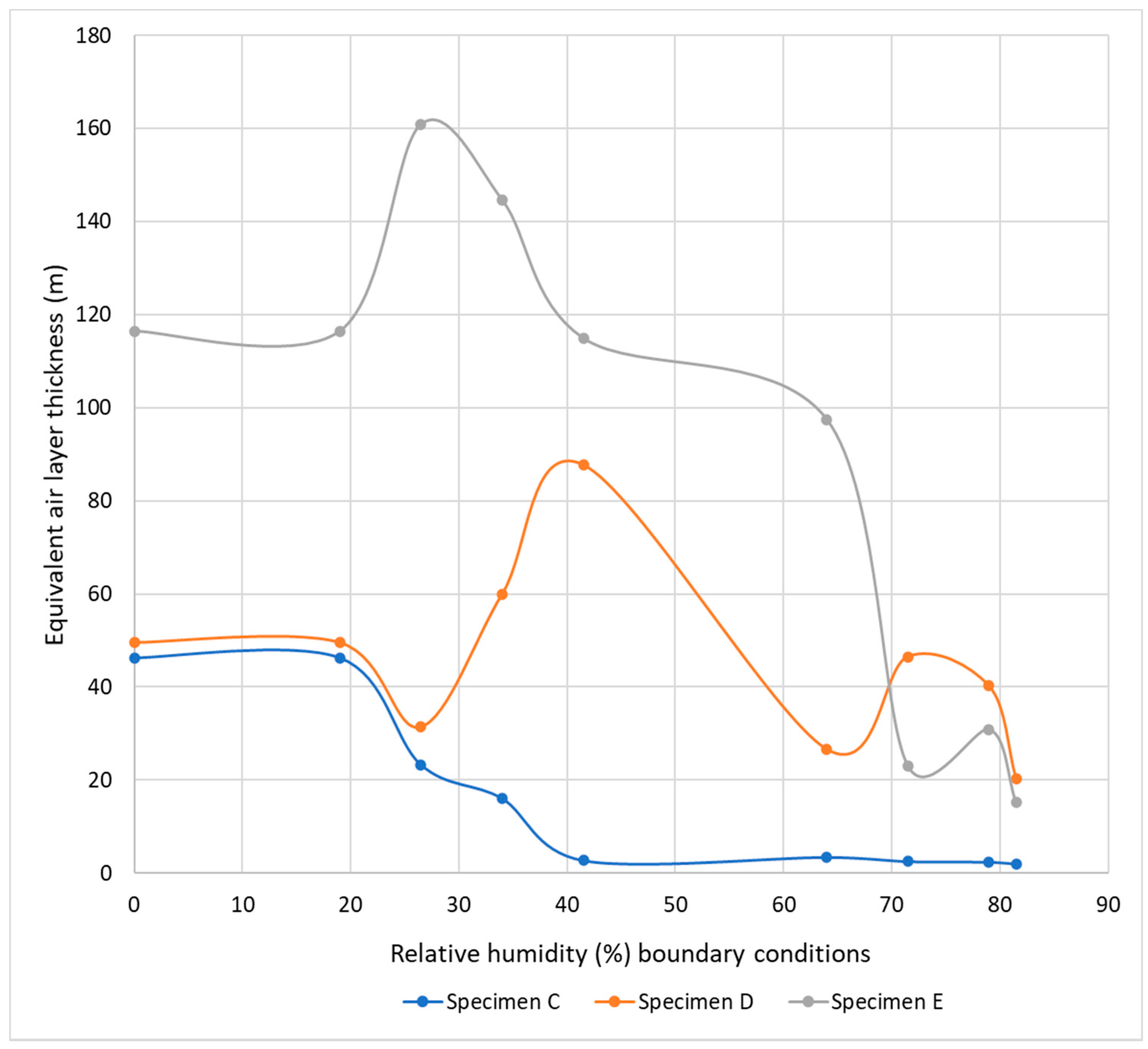
Temperature	Dry Side RH (%)	Wet Side RH (%)	Average RH (%)	Specimen C Sd (m)	Specimen D Sd (m)	Specimen E Sd (m)
23	3	35	19	46.21	49.5	116.4
23	3	50	26.5	23.25	31.4	160.8
23	3	65	34	16.04	59.9	144.6
23	3	80	41.5	2.72	87.7	114.9
23	35	93	64	3.4	26.6	97.5
23	50	93	71.5	2.5	46.5	23.07
23	65	93	79	2.37	40.19	30.9
23	80	93	81.5	1.98	20.3	15.2

shows the summary of hygrothermal water vapour resistance factor and equivalent air layer thickness across the boundary conditions over the average relative humidity for the three tested materials respectively, which were used to plot the hygrothermal boundary curves for specimen C, D, and E after harmonic adjustment.

4. Discussion

The aim of this research was to investigate the diffusion behaviour of water vapour impermeable, semi-impermeable, and permeable pliable membranes under different relative humidity boundary (moisture-dependent). This article focusses on the measured and calculated water vapour permeability values from two types of water vapour impermeable and one type of semi-impermeable membrane. A previous article reported the results from the measured and calculated water vapour diffusion properties of tested water vapour permeable membranes [13]. Firstly, it is important to state that this research successfully kept the temperature in the hygrothermal chamber stable at 23 °C with ±1 °C variation throughout all the four testing periods. Therefore, the shape of all the samples from the three tested pliable membranes observed was flat throughout the four testing periods, suggesting that there were no significant impact caused by temperature variation. Variation in temperature may alter the shape of membrane, which would affect the surface area calculations, which is very important when considering temperature-dependent measurement.

In Figure 1, the blue colour in the plot show the values for the water vapour resistance factor against the hygrothermal boundary conditions established from the average relative humidity conditions from the four laboratory measuring periods for Specimen C, which is classified as a class 2 (semi-impermeable membrane). In these measurements, the results indicate that the specimen was exposed to different relative humidities on both dry and wet sides. This difference in vapour pressure normally generates water vapour flow through the specimens, and as the humidity varies along the cross-section of the specimens, say from wet side to the dry, the vapour resistance also varies. Figure 1 shows that specimen C has different µ-values. From approximately 20% RH to 40% RH, the rate of water vapour diffusion varies significantly. Whilst from 40% RH to 80% RH, the water vapour diffusion rate is relatively constant. The vapour flow thus contains information about all the µ-values corresponding to the applied humidity interval as shown in Figure 2. This indicates that the water vapour diffusion resistivity properties of specimen C are non-linear as the amount of water vapour diffusion which passed through the specimen encounters different resistances, subject to the level of humidity. The graph also shows that the µ-values indicate an inverse relationship as the strength of the resistance factor decreased with increases in relative humidity.

Similar behaviour is observed from Figure 2, the blue colour is the plot of values of the equivalent air layer thickness against the established boundary conditions of the four experiment testing periods for specimen C. This also indicates that the water vapour flow across the cross-section of the specimen causes the equivalent air layer thickness to decrease in higher relative humidity, as the S_D value is high at lower relative humidity and lower in higher relative humidity in an inverse and dynamic pattern. Even though this dynamic behaviour is consistent with previous findings, it further supports the suggestion that the hygrothermal properties of construction materials should be considered under different relative humidity conditions. In Australia, hygrothermal diffusion function of pliable membrane is not yet defined under the current AS4200:1, and determining the appropriateness of pliable membranes according to their diffusion properties in different relative humidity conditions has become contestable among design professionals and researchers. Moreover, there are no appropriate and recent hygrothermal data for construction materials, typically used in Australia. Therefore, the ability to determine the hygrothermal boundary conditions of specimen C, with the resistance factor and equivalent layer thickness, is essential for accurately fulfilling the hygrothermal modelling pathway for moisture management introduced to NCC in 2019.

Similarly, the plot of the vapour resistance values against the relative humidity boundary condition for specimen D and E were indicated by the red colour and green, respectively, in Figure 1. The red and the green colour in Figure 2 also show the plot of equivalent air layer thickness against the humidity boundary conditions of specimen D and E respectively. Generally, impermeable pliable membranes usually have a very high vapour resistance factor and air layer equivalent thickness values as observed in Figure 2. However, it is essential to point out that even these graphs further document dynamic behaviour, similar to what this research has observed with other pliable membranes under varying relative humidity boundary conditions. The expectation was that these reflective impermeable pliable membranes would have a constant high resistance to water vapour diffusion. On the contrary, this did not occur as these reflective foil products have a rather unusual water vapour diffusion behaviour as the relative humidity conditions increased. The reason for the dynamic patterns observed in these graphs has resulted from the changes in air permeability and vapour pressure that has occurred under the four different relative humidity conditions. This level of water vapour diffusion resistance will cause these impermeable pliable membranes to have narrow usability potential for moisture-permeable construction systems.

As previously mentioned, measurements were usually taken weekly because of high water vapour diffusion resistance of these specimens. In this scenario, this research observed that when the specimens from the two types of reflective membranes were tested at 80% RH, the specimen were swelling within a week. Additionally, by the second week of weighing, there was a visible formation of mould growth on the reflective surface of all the specimens (see Figure 3 and Figure 4). The program for this research involved testing specimens from all the classes of pliable membranes at 80% RH during the same period. The yellow-brownish colouration of mould formation on these reflective materials was not observed on any of the other materials tested.

Comparing the result of these three membranes with each other, specimen C, which is semi-impermeable and belongs to Class 2, appears to be more open to vapour diffusion process with higher vapour resistance values when the humidity was less than 40%. Specimen D and E, which are classified as Class 1, impermeable pliable membranes, have very high vapour resistance factors and equivalent air layer thickness despite the increase in relative humidity conditions.

Harmonic Adjusment of Hygrothermal Boundary Curve

The cup measurements are used to determine the boundary condition of the water vapour diffusion characteristics of a material by plotting a curve after harmonic adjustment of the data from dry and wet cup gravimetric measurement. This is because there is the need to establish the different values of vapour diffusion at any given specified relative humidity ϕ, as the cup measurements do not directly provide these values. During the gravimetric measurement, the specimen is exposed to different relative humidities on both sides, for example, 50% on one side and 80% on the other side. The humidity varies continuously along the cross-section of the specimen, from 50% RH on one side to 80% RH on the other side, with all intermediate values also occurring somewhere in the specimen. Furthermore, the material in different parts of the specimen also has different µ-values, and all µ-values from µ (50%) to µ (80%) occur simultaneously somewhere in the specimen. However, the cup measurement can only tell us the strength of the vapour flow which diffused through the specimen. The vapour flow thus contains information about all the µ-values corresponding to the applied humidity interval, which are encoded in a single number. The task now is to determine µ-values for individual humidities. This can be done by combining the results of cup measurements using different humidity ranges. Hence, analysing gravimetric cup measurements as if the material had a constant µ-value, provides the effective µ-value of the specimen in such states of moisture. Therefore, the effective µ-value for a given humidity range is the harmonic mean of the µ(ϕ)-curve, taken over the humidity range. This is why it may be misleading to draw a µ(ϕ)-curve by simply plotting the effective µ-values against the mean applied humidity ranges from purely gravimetric measurement.

Figure 5 shows a µ(ϕ)-curve (grey) and a series of mean values (orange bars) of this curve, taken over humidity ranges with the same midpoint but with increasing widths. First, due to the curvature of the µ-curve, all those mean values are lower than the curve itself at the midpoint. The curve point is the desired µ-value corresponding to the midpoint humidity. The mean values correspond to the results of cup measurements performed by applying the respective humidity ranges. The results of all cup measurements are lower than the µ-curve point corresponding to the midpoint humidity, so it would be inappropriate to simply substitute a cup measurement result for this µ-value. Secondly, the mean values for humidity ranges with the same midpoint are lower for wider ranges. This means that when cup measurements with different wide humidity ranges are combined into one diagram (plotting them against the midpoint humidity), a misleading zigzag-shape of the diagram may result, even though the underlying true µ(ϕ)-curve may be continuously falling for increasing humidity.

A better approach than plotting the cup results against the midpoints of the applied humidity ranges is to determine a curve which has the properties that the harmonic mean values provide, taken over the humidity ranges which were used for the cup measurements, and are identical with the cup results. Figure 6 illustrates the procedure using data from WUFI for an adaptive vapour retarder, with the green bars representing a set of cup measurements, the grey curve being the adjusted test curve, and the thin orange bars being the mean values of the test curve, taken over the indicated ranges. The test curve is adjusted until the orange bars coincide as well as possible with the green bars.

The above principle was applied to the three materials measured in this research, to plot the final hygrothermal boundary curve for the equivalent air layer thickness for specimen C, D, and E (see Figure 7) after the harmonic adjustment. These harmonically balanced values could be applied to the material properties within the transient hygrothermal simulation software to provide a more accurate simulation of the water vapour diffusion through an external envelope.

5. Conclusions

This research has investigated through laboratory measurement the water vapour diffusion characteristics of two types of water vapour impermeable reflective pliable membranes and one type of smart membrane. The research included measuring their water vapour diffusion behaviour under varying boundary conditions, with specific attention to different relative humidity conditions.

The results from the cup measurements show that the two vapour impermeable pliable membrane products are not open to vapour diffusion even at higher relative humidity conditions, as their resistance factor and air layer thickness are too high to allow for vapour diffusion. On the other hand, the result from the smart pliable membrane product indicates that vapour diffusion is possible at higher relative humidity, as the resistance factor and air layer thickness decreases with increases in relative humidity. Contrary to the single point test method applied typically to construction materials, the graphs for all the three types of pliable membrane material show that they behave in a dynamic non-linear manner subject to the relative humidity conditions. This finding is similar in nature to the previously published findings which reported on the non-linear vapour diffusion properties for tested vapour permeable pliable membranes [13]. Alarmingly, the composite materials that make up the vapour impermeable pliable foil-faced membranes supported mould growth during the test period, whilst the non-foil polyethylene copolymer products did not support mould growth. Further analysis based on the harmonic adjustment approach was then employed to plot the hygrothermal boundary curves for each of these pliable membranes. This is because the results from the gravimetric cup measurement may not be enough to determine the effectiveness of a materials’ moisture behaviour along the cross-section of these materials, which is needed for hygrothermal modelling.

In conclusion, this research demonstrates that regardless of the water vapour diffusion class, each of the tested pliable membrane types behaved differently under different relative humidity conditions and vapour pressure gradients within the testing laboratory. This may indicate that the current single point value for construction material vapour diffusion properties used in hygrothermal simulation may be inadequate and may provide inaccurate guidance regarding moisture, moisture accumulation, and mould growth.

References

- Olaoye, T.S.; Mark, D. Establishing an Environmentally Controlled Room to Quantify Water Vapour Resistivity Properties of Construction Materials. In Revisiting the Role of Architecture for ‘Surviving’ Development; Avlokita, A., Rajat, G., Eds.; Architectural Science Association (ANZAScA): Roorkee, India, 2019; pp. 675–684. [Google Scholar]
- Olaoye, T.S.; Dewsbury, M.; Kunzel, H.; Nolan, G. An Empirical Measurement of the Water Vapour Resistivity Properties of Typical Australian Pliable Membrane. In Proceedings of the 54th International Conference of the Architectural Science Association (ANZAScA), Auckland, New Zealand, 25–28 November 2020. [Google Scholar]
- Künzel, H.M. Adapted Vapour Control for Durable Building Enclosures. In Proceedings of the 10th International Conference on Durability of Building Materials & Components, Lyon, France, 17–20 April 2005. [Google Scholar]
- Künzel, H.M.; Zirkelbach, D.; Sedlbauer, K. Predicting Indoor Temperature and Humidity Conditions Including Hygrothermal Interactions with the Building Envelope. In Proceedings of the 1st International Conference on Sustainable Energy and Green Architecture, Building Scientific Research Center (BSRC), King Mongkut’s University, Thonburi, Bangkok, 8–10 October 2003. [Google Scholar]
- Australia Building Code Board (ABCB). National Construction Code Ncc 2019 Building Code of Australia—Volume One; ABCB: Canberra, Australia, 2019. [Google Scholar]
- WHO. Who Guidelines for Indoor Air Quality: Dampness and Mould; WHO Regional Office for Europe: Copenhagen, Denmark, 2009. [Google Scholar]
- US EPA, IAQ. Moisture Control Guidance for Building Design, Construction and Maintenance; U.S. Environmental Protection Agency: Washington, DC, USA, 2013.
- Institute of Medicine IOM. Damp Indoor Spaces and Health; Institute of Medicine, National Academies Press: Washington, DC, USA, 2004. [Google Scholar]
- Maurice, D.; Lacasse, M.; Laouadi, A. A Comparison of Hygrothermal Simulation Results Derived from Four Simulation Tools. J. Build. Phys. 2021. [Google Scholar] [CrossRef]
- Maref, W.; Tariku, F.; Di Lenardo, B.; Gatland, S.D. Hygrothermal Performance of Exterior Wall Systems Using an Innovative Vapor Retarder in Canadian Climate. In Proceedings of the 4th International Building Physics Conference, Istanbul, Turkey, 15–18 June 2009. [Google Scholar]
- John, S.; Burnett, E. Review of Modeling Methods for Building Enclosure Design. Ph.D. Thesis, University of Waterloo, Waterloo, ON, Canada, 1999. [Google Scholar]
- John, C.; Roger, G.; Mavinkal, K.K. A Logical Extension of the Astm Standard E96 to Determine the Dependence of Water Vapour Transmission on Relative Humidity. In Insulation Materials: Testing and Applications, 3rd ed.; ASTM International: West Conshohocken, PA, USA, 1997. [Google Scholar]
- Samuel, T.; Dewsbury, M.; Künzel, H. Empirical Investigation of the Hygrothermal Diffusion Properties of Permeable Building Membranes Subjected to Variable Relative Humidity Condition. Energies 2021, 14, 4053. [Google Scholar]
- Valovirta, I.; Juha, V. Water Vapor Permeability and Thermal Conductivity as a Function of Temperature and Relative Humidity. In Proceedings of the IX International Conference, Oak Ridge, FL, USA, 5–10 December 2004. [Google Scholar]
- Bomberg, M.; Marcin, P. Methods to Check Reliability of Material Characteristics for Use of Models in Real Time Hygrothermal Analysis. In Proceedings of the First Central European Symposium on Building Physics, Lodz, Poland, 13–15 September 2010. [Google Scholar]
- Olaoye, T.S.; Mark, D. Australian Building Materials and Vapour Resistivity. In Building Physics Forum; AIRAH: Wollogong, Australia, 2018. [Google Scholar]
- AS/NZS. Pliable Building Membranes and Underlays. In AS/NZS 4200:1; Council of Standards Australia: Sydney, Australia, 2017. [Google Scholar]
- ASTM. Standard Test Methods for Water Vapor Transmission of Materials. In E96/E96M; ASTM International: West Conshohocken, PA, USA, 2010. [Google Scholar]
- ANSI/ASHRAE. Criteria for Moisture-Control Design Analysis in Buildings. In ASHRAE Standard 160; American Society of Heating, Refrigerating and Air-Conditioning Engineers: Atlanta, GA, USA, 2009. [Google Scholar]
- Künzel, H.M.; Daniel, Z. Advances in Hygrothermal Building Component Simulation: Modelling Moisture Sources Likely to Occur Due to Rainwater Leakage. J. Build. Perform. Simul. 2013, 6, 346–353. [Google Scholar] [CrossRef]
- Feldman, D. Polymer Barrier Films. J. Polym. Environ. 2001, 9, 49–55. [Google Scholar] [CrossRef]
- May-Britt, H. Membranes in Chemical Processing a Review of Applications and Novel Developments. Sep. Purif. Methods 1998, 27, 51–168. [Google Scholar] [CrossRef]
- Tabor, J.; Tushar, G. Building and Construction Textiles. High Perform. Tech. Text. 2019. [Google Scholar] [CrossRef]
- Lstiburek, J. Moisture Control for Buildings. ASHRAE J. 2002, 44, 36–41. [Google Scholar]
- ISO, International Standard Organization. Hygrothermal Performance of Building Materials and Products—Determination of Water Vapour Transmission Properties Cup Method Iso 12572. In EVS-EN ISO 12572:2016; Estonian Centre or Standardization: Brussels, Belgium, 2016. [Google Scholar]