Suitability of Seismic Isolation for Buildings Founded on Soft Soil. Case Study of a RC Building in Shanghai

Abstract

Base (seismic) isolation is a promising technology for seismic protection of buildings and other constructions. Nowadays, it is accepted that such a technique is efficient and reliable; however, it has two major limitations: soft foundation soil, and tall buildings. The first issue restrains the seismic isolation spreading, given that soft soil is frequent in densely populated areas, and usually such a soil type concentrates the highest seismicity levels. This paper aims to contribute to demonstrating that base isolation, if properly implemented, can be suitable for soft soil. A representative case study is analyzed: a 6-story reinforced concrete (RC) building with base isolation that has recently been built in Shanghai. Since the building is founded on soft soil, concern regarding base isolation suitability arose; even the Chinese design code does not recommend this solution for soft soil. To clarify this issue, non-linear time-history analyses are carried out for a number of natural and artificial seismic inputs that represent the site seismicity; the superstructure behavior is linear, while nonlinearities are concentrated in the isolation layer. The adequacy of base isolation is assessed in the superstructure (in terms of reduction of interstory drift, absolute acceleration and shear force) and in the isolation layer (in terms of axial force, torsion angle and shear strain). The relevance of soil–structure interaction is discussed. The behavior when the mechanical parameters of the isolation units have experienced important changes is also analyzed. The major conclusion is that base isolation of ordinary mid-height RC buildings founded on soft soil can perform satisfactorily in medium seismicity regions.

1. Introduction

Base (seismic) isolation consists in uncoupling the construction under consideration from the foundation soil by using bearings that are flexible in the horizontal direction, being commonly termed as isolators (or isolation units). The resulting structure is divided into three parts: superstructure, isolation layer, and substructure; ordinarily, the isolation layer is situated right below the ground floor slab. Base isolation has been mainly considered for buildings and bridges; this study deals with seismically isolated buildings. The main effect of seismic isolation of buildings is an important elongation of their fundamental period, thus reducing significantly the spectral ordinate. Moreover, given that most of the drift displacement is concentrated in the isolation layer, additional damping can be easily incorporated; as a result, the spectral ordinate is further lowered.

The suitability of base isolation has been repeatedly proven by theoretical studies, laboratory testing, and observation of the seismic performance of actual buildings under strong seismic events. Therefore, nowadays such technology is recognized worldwide, being incorporated into the major design codes. However, although seismic isolation performs satisfactorily in most of the situations, it has two major limitations: high-rise buildings, and soft foundation soil. This paper deals with the second limitation; this choice is based on the important number of buildings in high seismicity regions that are founded in soft soil. Analyzing this limitation in more depth, it is widely accepted that base isolation is less efficient for soft soil [1,2,3,4,5]; the main reason for this prevention is that soft soil filters out short-period waves while it amplifies long-period components. Therefore, given the similarity between the wave predominant periods and the fundamental period of the isolated building, the ground motion in the superstructure could prove enlarged, instead of reduced. Several previous studies on this subject have been published [6,7,8,9,10,11].

Many design codes discourage the use of base isolation in soft soil [12,13,14]; sometimes, simplified design methods (equivalent static forces) are prevented, thus requiring the employment of more general strategies, typically non-linear time-history analysis [14]. This paper analyzes a representative case study, this being an isolated building in Shanghai; the particular interest of this case for China is discussed next.

The Wenchuan earthquake (12 May 2008) caused numerous casualties, principally students. Thereafter, concerns about the seismic safety of teaching buildings arose in China. In the Lushan earthquake (20 April 2013), a base-isolated hospital building experienced only minor damage and played a significant role in rescue work [15]; then, a broad pilot study on the seismic isolation of teaching buildings was undertaken. In the framework of this research effort, this paper investigates the rationality of using base isolation for buildings founded on soft soil. The aim is developing a strategy of verification and analyzing a relevant case study; no similar studies have been found in the technical literature.

The case study is a 6-story RC (reinforced concrete) building with rubber isolators and viscous dampers that had been recently constructed in Shanghai [16,17]. The building had been designed for seismic intensity degree 7 according to the current Chinese code [12], whose design input peak accelerations are 0.10 g and 0.22 g for moderate and rare earthquakes, respectively. Moderate and rare earthquakes correspond to a 10% and 2% possibility of being exceeded in 50 years, respectively. Given that the building is founded on soft soil, concern regarding the suitability of using base isolation arose; noticeably, the Chinese code [12] does not recommend this solution for that soil condition. This paper evaluates numerically the seismic performance of the isolated building; therefore, the study refers only to the after-construction stage. The performance is assessed through non-linear time-history analyses of the building being shaken by a number of seismic inputs; such analyses are performed with the software SAP2000 v16.0 [18]. These input accelerograms are selected to represent the site seismicity, mainly accounting for the soil conditions. In the analyses, the behavior of the superstructure is modelled as linear, while nonlinearities are concentrated in the isolation layer. The need for considering soil–structure interaction (SSI) is discussed, and SSI numerical simulations are carried out. Notably, given that the objective of the paper is to investigate the suitability of base isolation in buildings founded on soft soil, other soil types are not considered.

The adequacy of base isolation is assessed in both the superstructure and the isolation layer. In the superstructure, the appropriateness of base isolation is judged in terms of the reduction of interstory drift, absolute acceleration, and shear force. In the isolators, the correctness is evaluated in terms of axial force and lateral displacement (shear strain); for this purpose, the prescriptions of the Chinese code [12] and the European regulations for base isolation [19,20] and for rubber bearings [21] are considered.

2. Building under Consideration

2.1. Superstructure

The structure of the analyzed building is a RC frame; there are no shear walls or other structural or non-structural members that might provide significant lateral stiffening or strengthening. The building has six stories and one basement; the isolators are placed at the ground level, i.e., on the top of the basement columns. Figure 1 represents the analyzed building; Figure 1a displays a 3-D rendered view and Figure 1b exhibits a picture. Figure 1c,d refers to a typical floor plan layout; Figure 1c shows the architectural distribution and Figure 1d represents the structural configuration, indicating columns (black squares) and beams.

Figure 1 shows that the plan area is rectangular, and the configuration is essentially regular; as shown in Figure 1a, the building width, depth and height are 58.5 m, 18.3 m and 22.95 m, respectively. The columns have a constant rectangular cross section ranging between 60 cm × 70 cm (inner columns) and 90 cm × 90 cm (corner columns). The slabs are formed by rectangular beams that are 30 to 35 cm wide and 50 to 70 cm deep, and constant-depth slabs being 11 to 14 cm deep. The characteristic value of the concrete compressive strength is f_ck = 30 MPa and the deformation modulus is estimated as E_c = 30 GPa. The reference [16] contains deeper information on the structural parameters. The live (variable) gravity load is established according to the Chinese design code [22], ranging between 2 and 2.5 kN/m², except for stairs and other highly crowded areas. The seismic weight corresponds to the combination D + 0.5 L where D and L account for dead (permanent) and live (variable) loads, respectively. For this loading level, the building mass is 9576 t; from the first to top (6th) floor, the masses are 1569, 1652, 1607, 1621, 1854 and 1273 t, respectively. To analyze the influence in the plan symmetry of irregular columns arrangements and other unevenness (e.g., balconies), the eccentricities between the mass and rigidity centers of each floor are determined: in the x direction, the eccentricity ranges between 0.15% (first floor) and 0.70% (top floor) while in the y direction, it ranges between 3.75% (top floor) and 5.14% (first floor).

2.2. Isolation Layer

The isolation system is formed by the parallel combination of rubber bearings (isolation units) and viscous dampers; the sought damping ratio considers the recommendations in [23]. Two types of isolator are employed: ordinary natural rubber bearings and lead-rubber bearings, i.e., incorporating a central lead plug core to provide additional damping. Those devices are termed in this paper NRB (natural rubber bearing) and LRB (lead rubber bearing), respectively.

The rubber shear modulus is G = 0.392 N/mm² for all the devices;

Table 1. Rubber bearing parameters.

Name	Diameter (mm)	Height (mm)	Rubber Layer Height (mm)	Rubber Height (mm)	Lead Plug Diameter (mm)	Horizontal Stiffness (kN/m)	Critical Shear Strain/Stress (%/MPa)	Yielding Force (kN)	After-Yielding Horizontal Stiffness (kN/m)
NRB700	700	451.5	5	200	-	742	280/8	-	-
NRB800	800	438.5	6	204	-	951	301/10	-	-
LRB700	700	451.5	5	200	160	1565	282/8	160	764
LRB800	800	438.5	6	204	160	1758	304/10	160	972

displays the other main geometric and mechanic parameters of the rubber isolators.

Two types of viscous damper are installed in the x and y directions, respectively;

Table 2. Parameters of the viscous dampers.

Direction	Exponent α	Initial Stiffness (kN/mm) *	Maximum Stroke (mm)	Damping Coefficient c (kN/(mm/s)0.4)	Speed (mm/s)	Maximum Damping Force (kN)	Design Life (Years)
x	0.4	49	±350	70	600	900	50
y	0.4	42	±350	60	600	800	50

* Elastic combined axial stiffness of the supporting brace and internal damper portion.

displays their major parameters. Section 3.2 describes the meaning of such parameters.

Figure 2 contains pictures and sketches of the installation of the rubber bearings and the viscous dampers. Figure 2a,b represent a pair of isolators and a damper, respectively; Figure 2b shows that the viscous dampers are installed (between two adjoining isolators) connecting the ground floor slab (superstructure) with the basement columns (substructure). Figure 2c displays the plan layout of isolators and dampers. Figure 2c shows that isolators and dampers are arranged symmetrically; as well, dampers and LRBs (bearings with lead plugs) are located near the building perimeter, thus providing torsion damping and stiffness.

2.3. Soil and Foundation

As the soil is soft, the building is founded on piles. Each pile is 600 mm in diameter and 28 m deep. The bedrock in Shanghai is often located 200~300 m underground, being covered by thick quaternary unconsolidated sediments. For categorization purposes, the soil is divided into 9 layers, and each layer is split into several sub-layers. At the bottom of the piles (28 m depth), the soil condition is classified as layer 7-1, “grey clay silt”; the weighted harmonic average shear wave velocity down to 30 m (v_s30) ranges between 84 and 256 m/s [24]. For the seismic design, the soil is categorized as type IV; this is the softest class, according to the Chinese code [12]. Section 3.3 discusses more deeply the ground parameters that are relevant to the soil–structure interaction.

3. Numerical Modeling of the Isolated Building Dynamic Behavior

3.1. Model of the Superstructure

The building lateral dynamic behavior is described with a linear 3D model implemented in the SAP2000 v16.0 software package [18]. Beams and columns are represented by frame elements, and slabs are modeled with shell elements. The rigid diaphragm effect is indirectly considered by the high in-plane stiffness of slabs. The stiffness of the members is determined based on their gross sectional parameters, although reduced to account for cracking; the corresponding reducing coefficient is 0.5 for beams, and 1 for columns and slabs [25]. Noticeably, that reduction is unnecessary in the Chinese code [12]. Figure 3 displays an overview of the building model. The damping is described by a classical Rayleigh model; the mass and stiffness coefficients are selected for a damping ratio 0.05 in the first two modes.

3.2. Model of Isolators and Dampers

The behavior of the natural and lead-rubber bearings is described by linear and hysteretic bilinear models, respectively. Table 1 displays the main parameters of both models; their torsional stiffness is neglected.

Regarding the dampers, their behavior is represented by a nonlinear viscous damping model:

$$f=c {\dot{x}}^{\mathsf{\alpha }}$$

(1)

In Equation (1), f represents the damper force; the values of the damping coefficient c and the exponent α are listed in Table 2. Equation (1) can be considered as a modification of the classical linear Maxwell model [26,27], where the stiffness coefficient has been neglected.

3.3. Soil–Structure Interaction Modelling

A number of studies on the relevance of SSI in base-isolated buildings have been reported [6,8,9,11,28,29,30]. These studies conclude that the consideration of SSI is not necessary, unless the soil is very soft and the building is relatively stiff; moreover, commonly, the SSI effect is rather beneficial. Therefore, the above studies seem to indicate that, given the high lateral flexibility of the isolated building, SSI might be neglected. However, for the sake of safety, a simplified SSI study is performed herein. SSI is described with an uncoupled linear spring model [31]; such a model consists in representing the interaction by six springs that connect each pile cap to the adjoining soil.

The axial stiffness of each pile is calculated by two approaches: (a) it is assumed that the piles rest on a rigid bedrock, therefore, their stiffness is E_p A_p/L_p (E_p, A_p and L_p refer to modulus of deformation, cross section area and length of the pile, respectively), and (b) since the piles do not actually reach the bedrock, only the friction stiffness is accounted for. In this last case, the vertical stiffness K_vf of a pile can be calculated by the formulation proposed in [32]:

$$K_{\mathrm{vf}}=1.8 E_{\mathrm{s}} D_{\mathrm{p}} {\mathsf{\lambda }}^{0.55} {\mathsf{\eta }}^{-b}$$

(2)

In Equation (2), E_s is the soil modulus of elasticity, D_p is the pile diameter, λ is the ratio between the pile length and diameter (λ = L_p/D_p), η is the ratio between the soil and pile moduli of elasticity (η = E_p/E_s), and the exponent b is given by b = λ/η. In the analyzed case, E_p = 26 GPa, L_p = 28 m, D_p = 0.60 m, and E_s is calculated after the shear modulus G_s based on the weighted average shear wave velocity (v_s) and the soil density (ρ_s) on the top 28 m.

Table 3. Parameters of the soil layers in the top 28 m.

Layer Type	Cumulated Depth (m)	Density (kg/m3)	Shear Wave Velocity (m/s)
Filled earth	4.2	1870	112
Muddy-silty clay	9.5	1820	128
Muddy clay	22.5	1760	178
Muddy-silty clay	32.8	1800	245

displays the soil properties of each layer in the top 28 m:

Table 3 shows that, in this case, the average values of the shear wave velocity and density are v_s = 171.8 m/s and ρ_s = 1795 kg/m³, respectively; therefore: G_s = 53 MPa, and, by assuming that the Poisson ratio is ν = 0.25, E_s = 132.5 MPa. Finally, E_p A_p/L_p = 263 kN/mm and K_vf = 338 kN/mm; thus, the friction stiffness (K_vf) is 1.29 times higher than the axial one (E_p A_p/L_p), what is consistent with the estimations in [33]. Finally, for each cap, the vertical spring stiffness is obtained as the sum of those of each pile.

The rotational stiffness with respect to the horizontal axes are determined, from the vertical stiffness of each pile, by equilibrium conditions. For each cap, the torsional and horizontal stiffness are determined, in terms of the soil parameters and foundation dimensions, as indicated in [34]. The soil damping effect is neglected; this is a conservative assumption, since it would decrease the base shear force.

4. Modal Analysis of the Building

Linear modal analyses of the building under fixed-base and isolation conditions are carried out by using the models described in the previous section.

Table 4. Modal parameters of the building under fixed-base/isolated conditions.

Mode No.	Period (s)	Modal Mass Factor x	Modal Mass Factor y	Modal Mass Factor φ
-/1	-/3.586	-/0.046	-/0.910	-/0.03561
-/2	-/3.528	-/0.940	-/0.053	-/0.0039
-/3	-/2.983	-/0.011	-/0.029	-/0.96049
1/4	1.229/0.571	0.010/7.25 × 10−7	0.717/0.004	0.074/1.142
2/5	1.163/0.502	0.621/2.29 × 10−3	0.046/1.02 × 10−6	0.156/2.23 × 10−6
3/6	1.106/0.177	0.196/7.08 × 10−8	0.037/0.39 × 10−6	0.569/8.59 × 10−8

displays the periods and modal mass ratios of the first six modes of the base-isolated building, and of the first three modes of the fixed-base building; φ accounts for twist angle (torsion). Given that the incorporation of the isolation layer adds three new modes, in Table 4 the first three modes of the fixed-base building are associated with the 4th, 5th and 6th modes of the base-isolated building, respectively. In the isolated building, the periods are calculated for the effective secant stiffness (of the lead-rubber isolators) that correspond to 100% shear strain. In Table 4, the highlighted values correspond to the biggest component of each mode, in terms of modal mass factor.

Table 4 provides the following remarks:

▪

Fixed-base building. The first mode corresponds basically to motion along the y direction (also some torsion), the second mode involves motion along the x direction (there is torsion as well), and the third mode contains mainly torsion. The relatively long period of the third mode (1.106 s) indicates a low torsional stiffness; this is coherent with the absence of any important stiffening element in the façades. Therefore, further verifications are carried out. The simplified expression for regular reinforced concrete frames that are contained in the European [19] and American [35] codes (among others) provide a fundamental period equal to 0.676 s; since the building is rather flexible (as base isolation allows for significant reductions in the lateral design forces), the difference among this value and those in Table 4 is feasible. For further verification, the building has been also modelled with the PKPM Chinese software code [36]; the obtained periods are highly similar to those from SAP.

▪

Base-isolated building. The first three modes correspond basically to motion along the y, x and φ directions, respectively. Such modes gather most of the mass; this indicates a rather satisfactory performance of base isolation, since those modes correspond basically to rigid-body motion (i.e., without any structural damage).

▪

Fixed-base vs. base-isolated building. Comparison among the periods of the first three modes of the base-isolated building and those of the fixed-base building shows that base isolation elongates the periods as expected. Similar comparison among the modal mass factors shows that the base-isolated building vibrates more symmetrically; this can be read as a proper design of the isolation system, in the sense that the slight plan asymmetry of the fixed-base building is corrected in the isolated solution.

Table 5. Modal parameters of the base-isolated building considering and without considering soil–structure interaction (SSI).

Mode No.	Period (s)			Modal Mass Factor x			Modal Mass Factor y			Modal Mass Factor φ
	SSI-a	SSI-b	No SSI	SSI-a	SSI-b	No SSI	SSI-a	SSI-b	No SSI	SSI-a	SSI-b	No SSI
1	3.603	3.608	3.586	0.032	0.053	0.046	0.942	0.877	0.910	0.023	0.067	0.036
2	3.544	3.540	3.528	0.957	0.922	0.940	0.036	0.067	0.053	0.004	0.008	0.004
3	2.892	3.178	2.983	0.008	0.022	0.011	0.018	0.052	0.029	0.972	0.921	0.961
4	0.443	0.661	0.571	0.002	-	-	-	0.003	0.004	-	-	-
5	0.306	0.600	0.502	-	0.002	-	0.004	-	-	0.001	0.001	-
6	0.193	0.580	0.177	-	0.001	-	-	-	-	-	0.003	-

displays the periods and modal mass ratios of the first six modes of the base-isolated building; such information is obtained for two conditions: by considering and neglecting SSI (Section 3.3). In Table 5, the values of the mass ratio that are smaller than 10⁻³ are indicated as “-”; SSI-a and SSI-b correspond to the consideration of axial and friction stiffness of the piles, respectively (Section 3.3). As in Table 4, the highlighted values correspond to the biggest component, in terms of modal mass factor, of each mode. Table 5 shows that the influence of SSI on the periods and modal mass ratios of the first three modes can be ignored. Also, comparison between both models of SSI shows little influence of the vertical stiffness of piles; therefore, the SSI results are reliable.

5. Seismic Inputs for the Dynamic Analyses

Representative accelerograms are selected according to the former and current Shanghai design codes [37]. Two sets of seven trios of accelerograms (i.e., in two horizontal directions and in vertical direction) are chosen. Each set is composed of five natural earthquake records and two artificial inputs; the records are taken from the PEER database [38], and the artificial inputs are created by modifying recorded accelerograms. The accelerograms of the first set correspond to soil with predominant period 0.9 s and are scaled to 1 m/s² (moderate earthquake); for the second set, the soil period is 1.1 s and the acceleration is 2.2 m/s² (rare earthquake).

Table 6. Seismic inputs for soil predominant period 0.9 s and scaled to maximum acceleration 1 m/s².

Code	Earthquake	Date	Mw	Hypocentral Depth (km)	Station	Component		PGV (m/s)	PGD (cm)	IA (m/s)	ID	Trifunac Duration (s)	Closest Distance (km)	Hypocentral Distance (km)	vs30 (m/s)
NR0.9-3	Kocaeli, Turkey	17-08-1999	7.51	15.0	USAK	x	USK090	0.272	4.831	0.451	10.36	35.52	226.7	237.0	274.5
						y	USK180	0.310	7.700	0.264	5.32	35.36
NR0.9-4	Hector Mine, USA	16-10-1999	7.13	5.0	San Bernardino Fire Station #9	x	0688c090	0.262	3.967	0.317	7.56	20.44	108.0	114.8	271.4
						y	0688a360	0.123	7.532	0.280	14.22	28.10
NR0.9-5	Denali, USA	03-11-2002	7.9	4.9	Anchorage New Fire Station #7	x	1734090	0.262	3.967	0.499	11.89	31.72	275.9	296.55	274.5
						y	1734360	0.228	2.060	0.561	15.37	29.80
NR0.9-6	Chichi, Taiwan	20-09-1999	6.02	18.0	CHY039	x	CHY039-N	0.197	14.260	0.349	11.06	35.70	46.8	52.53	201.2
						y	CHY039-E	0.244	18.919	0.299	7.65	36.72
NR0.9-7	Chichi, Taiwan	20-09-1999	7.62	18.0	CHY059	x	CHY059-N	0.185	14.162	0.398	13.44	38.56	86.3	88.53	191.1
						y	CHY059-E	0.190	6.717	0.361	11.87	33.94
AW0.9-2	Loma Prieta, USA	18-10-1989	6.93	17.5	Foster City Menhaden Court	x	MEN270	0.272	2.138	0.317	7.28	22.08	45.4	68.0	126.4
						y	MEN360	0.242	2.211	0.308	7.95	20.10
AW0.9-1	Hokkaido, Japan	29-11-2004	7.1	48	HKD085	x	HKD085EW	0.274	2.127	0.344	7.84	41.68	98.1	-	150.0
						y	HKD085NS	0.242	2.762	0.183	4.72	33.04

and

Table 7. Seismic inputs for soil predominant period 1.1 s and scaled to maximum acceleration 2.2 m/s².

Code	Earthquake	Date	Mw	Hypocentral Depth (km)	Station	Component		PGV (m/s)	PGD (cm)	IA (m/s)	ID	Trifunac Duration (s)	Closest Distance (km)	Hypocentral Distance (km)	vs30 (m/s)
NR1.1-3	Imperial Valley, USA	15-10-1979	7.62	10.0	El Centro Array #12	x	H-E12140	0.443	25.937	1.390	8.91	19.38	17.9	33.5	196.9
						y	H-E12230	0.284	20.607	0.975	9.75	19.14
NR1.1-4	Chichi, Taiwan	20-09-1999	7.62	6.8	CHY058	x	CHY058-E	0.467	34.299	3.615	21.97	45.64	59.8	91.4	237.6
						y	CHY058-N	0.490	32.451	2.896	16.78	45.88
NR1.1-5	Chichi, Taiwan	20-09-1999	7.62	6.8	CHY090	x	CHY090-E	0.446	28.146	2.917	18.57	38.78	58.4	89.8	201
						y	CHY090-N	0.556	40.618	2.569	13.12	45.32
NR1.1-6	Chichi, Taiwan	20-09-1999	7.62	6.8	KAU008	x	KAU008-E	0.575	68.312	3.230	15.95	46.06	107.0	143.7	285.9
						y	KAU008-N	0.633	57.951	3.054	13.70	46.06
NR1.1-7	Chichi, Taiwan	20-09-1999	7.62	6.8	KAU058	x	KAU058-E	0.584	76.979	3.172	15.42	40.16	107.8	143.3	201
						y	KAU058-N	0.717	72.504	4.263	16.88	46.84
AW1.1-2	Morgan Hill	24-04-1984	6.19	8.5	Foster City APEEL 1	x	A01040	0.450	55.382	1.528	9.64	26.82	53.9	55.0	116.4
						y	A01310	0.552	50.816	1.558	8.01	26.56
AW1.1-1	Hokkaido, Japan	26-09-2003	8.0	42	HKD066	x	HKD066EW	0.423	34.131	1.202	8.07	39.74	226.5	-	116.1
						y	HKD066NS	0.396	45.887	1.756	12.59	45.56

display the main features of both sets, respectively; the information in such Tables is described next. In the left column, “NR” accounts for “Natural Record” while “AW” means “Artificial Wave”. x/y directions correspond to strong/weak components, respectively. PGV and PGD refer to Peak Ground Velocity and Displacement, respectively. I_A is the Arias intensity [39] given by $I_{\mathrm{A}}=\frac{\mathsf{\pi }}{2 g}\int {\ddot{x}}_{\mathrm{g}}^2 dt$, where ${\ddot{x}}_{\mathrm{g}}$ is the input ground acceleration; the Arias intensity is an estimator of the input severity. I_D is the dimensionless seismic index [40] given by $I_{\mathrm{D}}=\frac{\int {\ddot{x}}_{\mathrm{g}}^2 dt}{PGA PGV}$; I_D accounts for the relevance of the velocity pulses. The Trifunac duration is the elapsed time between 5% and 95% of the Arias intensity I_A [41]. The closest distance corresponds to the shortest way to the rupture surface. The hypocentral distance is the straight separation between the hypocentre and the recording station. v_s30 is the harmonic weighted average shear wave velocity in the top 30 m; this parameter characterizes the soil type.

The natural records in Table 6 and Table 7 are selected based on the similarity between their individual response spectra and the code design spectra. Figure 4 displays response spectra of natural selected inputs (grey line) together with the code design spectrum (black line). Noticeably, all the spectra in Figure 4 correspond to records scaled to 1 m/s²; therefore, the plots in Figure 4c,d are reduced by a factor of 2.2. Figure 4 shows a rather satisfactory fit between the spectra of the scaled inputs and the code spectrum, particularly in the main (x) direction.

The artificial inputs are generated to fit the design spectrum, according to [12]. The fitting is established through 100 control points with logarithmic distribution in the interval [2 Δt, 10 s], where Δt = 0.02 s. The tolerance is 5%, in terms of quadratic error.

6. Time-History Analysis

6.1. Global Description of the Analyses

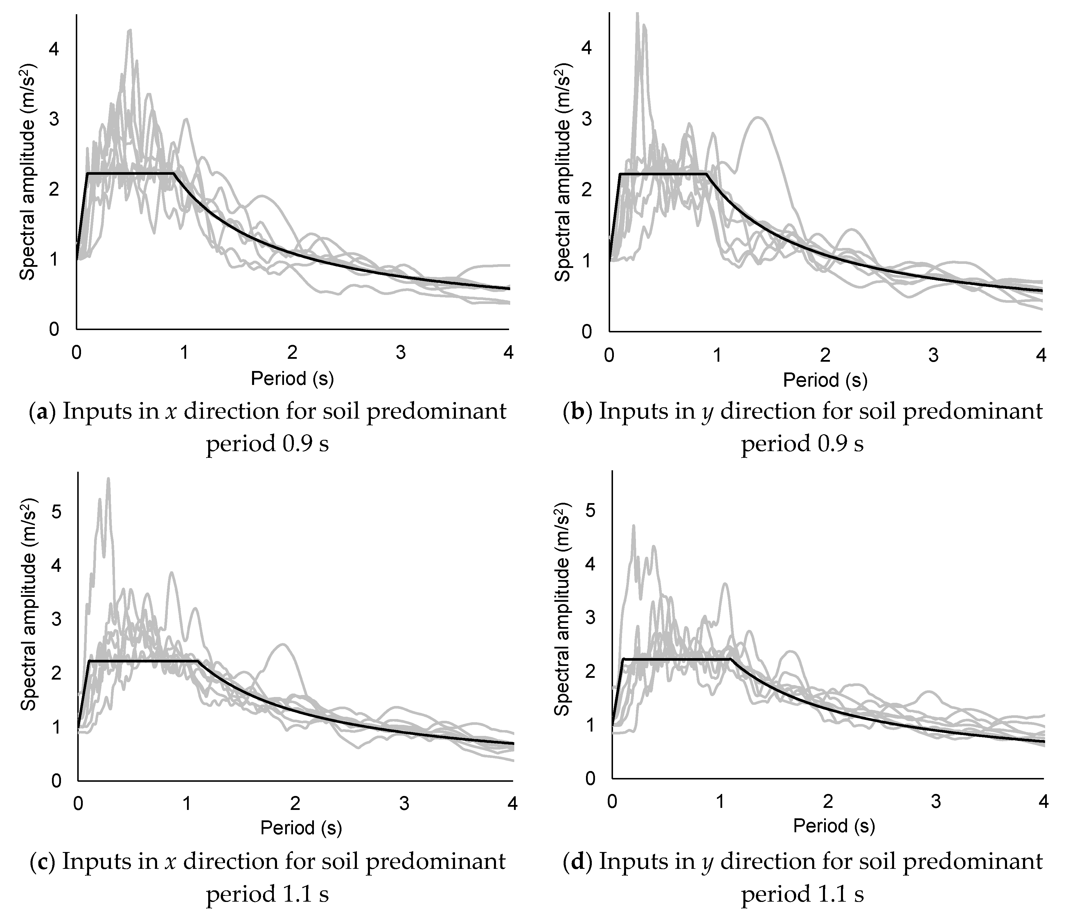
This section discusses the results of the time-history analyses for the inputs described in Section 5; the x/y input components are applied in x/y directions (Figure 2), respectively. As discussed in [42], the most meaningful results in the superstructure are the drift angle, shear force and absolute acceleration; in the isolators, the axial forces, shear strain and torsion angle are also significant.

The dynamic analyses are performed by implementing the numerical model described in Section 3 in SAP2000 v16.0 software package [18]. The building (superstructure) behavior is linear, the non-linearities are concentrated in the isolation layer. The analyses consider the simultaneous actuation of both horizontal input components. The time integration is performed using non-linear modal analysis; the time step is Δt = 0.02 s. The second-order effects have not been considered; it is observed that such effects do not over-magnify the relative displacements in the isolators, although can increase the moments significantly, sometimes more than 10%. It should be kept in mind that any numerical model is always affected by epistemic (and random) uncertainties as discussed in [43,44].

6.2. General Overview of the Results

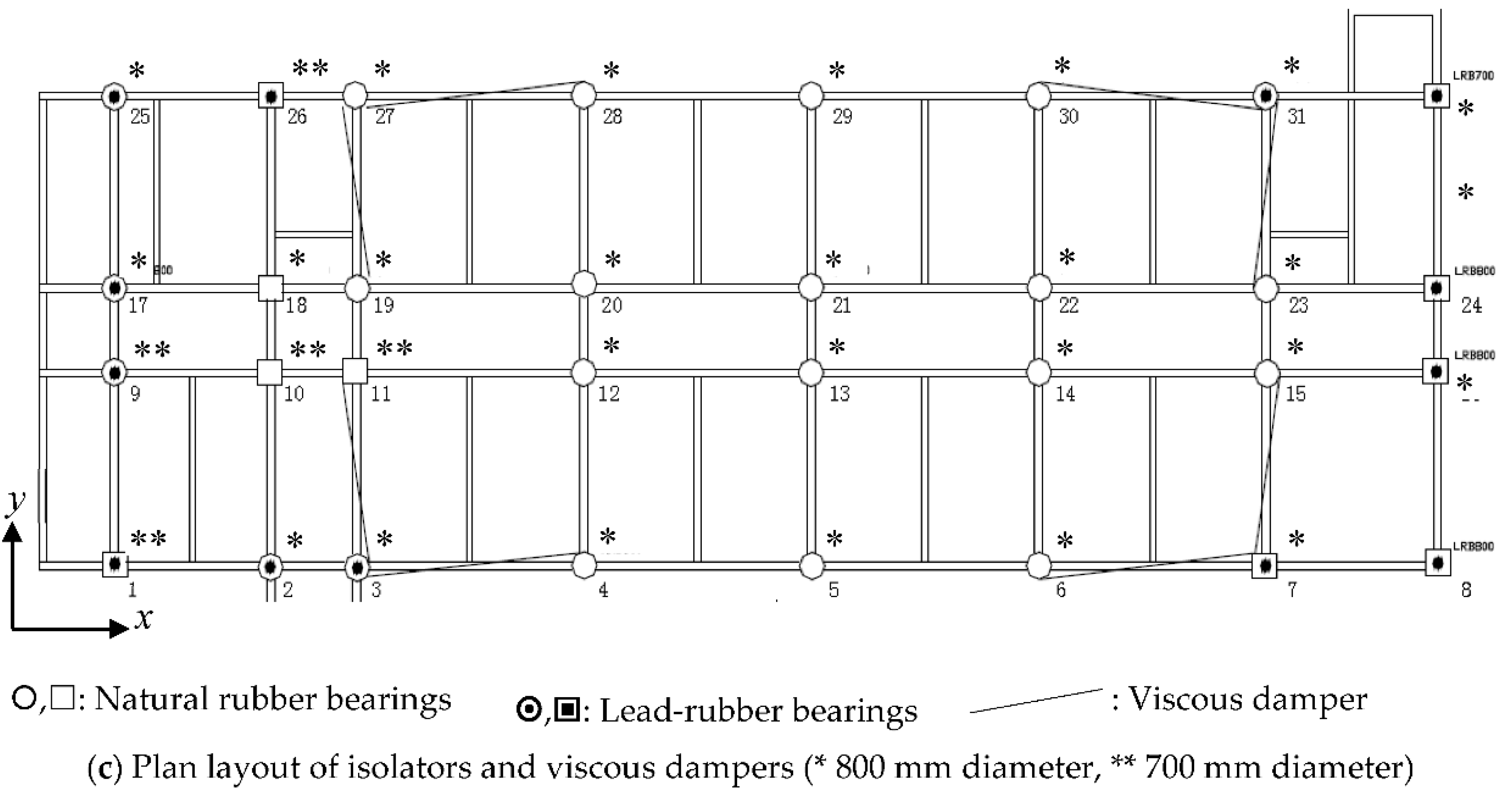
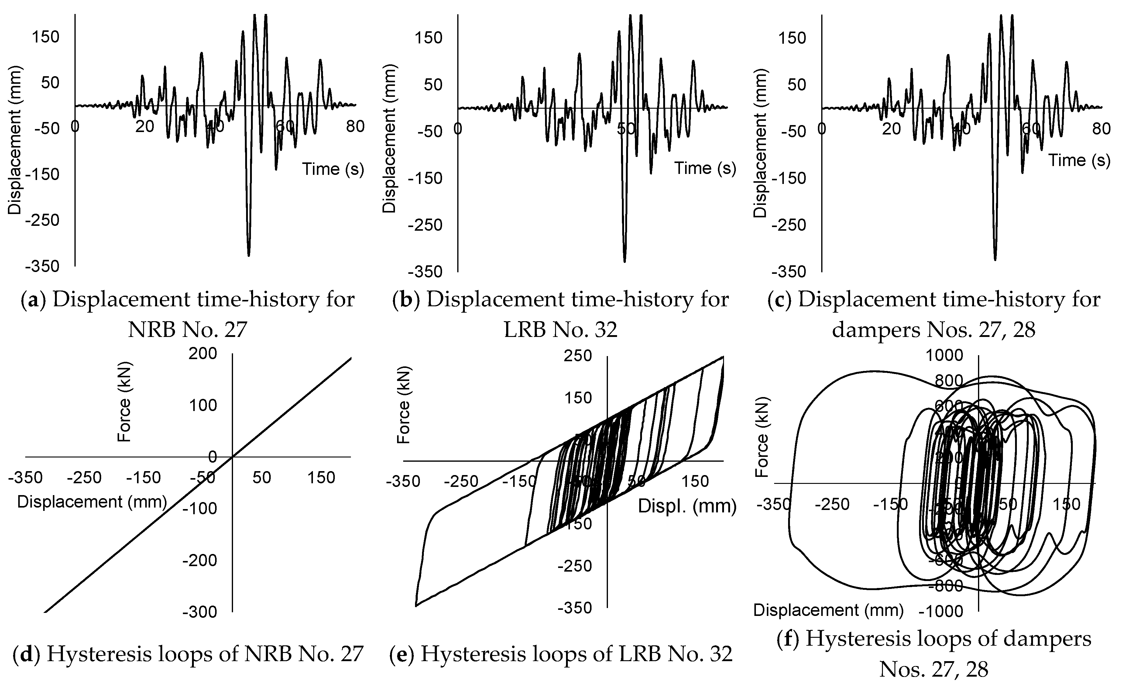
Figure 5 displays representative displacement time-history responses, and hysteresis loops of a natural rubber bearing (Figure 5a,d), a lead-rubber bearing (Figure 5b,e), and a viscous damper (Figure 5c,f); the labeling of isolators and damper refers to Figure 2c. All the plots in Figure 5 correspond to the input NR1.1-7 in the x direction (Table 7). Figure 5 shows a regular behavior; the similarity among the time-history plots in Figure 5a–c confirms the rigid diaphragm effect of the ground floor slab. On the other hand, the hysteresis loops in Figure 5d indicate a linear behavior, without any encompassed area; the loops in Figure 5e have almost quadrilateral shape, typical of the plastification of metals. Finally, the shape of the hysteresis loops in Figure 5f is closer to a rectangle than to an ellipse, this being consistent with the value of exponent α (α = 0.4, Table 2).

Under fixed-base and base isolation conditions,

Table 8. Average maximum * response values for the records NR0.9-3, NR0.9-6 and AW0.9-1 (Table 6).

Story	Input Direction	Drift Angle (%)		Shear Force/Supported Weight		Absolute Acceleration/Input Acceleration
		Fixed-Base	Base Isolation	Fixed-Base	Base Isolation	Fixed-Base	Base Isolation
Ground	x	-	22.0 **	-	0.042	1	1.035
	y	-	42.5 **	-	0.052	1	1.034
	x + y	-	46.5 **	-	0.059	1	1.124
1	x	0.306	0.161	0.147	0.054	1.178	0.726
	y	0.247	0.193	0.122	0.058	0.963	0.745
	x + y	0.350	0.219	0.170	0.069	1.088	0.749
2	x	0.472	0.160	0.174	0.054	1.347	0.481
	y	0.452	0.219	0.134	0.058	1.031	0.569
	x + y	0.559	0.240	0.197	0.072	1.230	0.543
3	x	0.464	0.133	0.200	0.054	1.405	0.438
	y	0.468	0.195	0.147	0.058	1.277	0.530
	x + y	0.553	0.210	0.221	0.069	1.399	0.513
4	x	0.408	0.106	0.222	0.054	1.819	0.580
	y	0.410	0.157	0.159	0.058	1.517	0.615
	x + y	0.486	0.169	0.241	0.070	1.758	0.607
5	x	0.277	0.068	0.238	0.055	2.188	0.694
	y	0.296	0.108	0.170	0.059	1.721	0.736
	x + y	0.340	0.114	0.257	0.071	2.041	0.696
6	x	0.147	0.036	0.262	0.059	2.426	0.762
	y	0.176	0.063	0.188	0.062	1.923	0.831
	x + y	0.192	0.066	0.282	0.076	2.242	0.774

* “Maximum” refers to along the input duration. ** Drift displacement divided by rubber height (shear strain).

and

Table 9. Average of maximum * response values for the records NR1.1-5, NR1.1-7 and AW1.1-1 (Table 7).

Story	Input Direction	Drift Angle (%)		Shear Force/Supported Weight		Absolute Acceleration/Input Acceleration
		Fixed-Base	Base Isolation	Fixed-Base	Base Isolation	Fixed-Base	Base Isolation
Ground	x	-	128.0 **	-	0.095	1	0.763
	y	-	132.0 **	-	0.105	1	1.035
	x + y	-	168.5 **	-	0.126	1	0.947
1	x	0.772	0.308	0.379	0.103	1.215	0.568
	y	0.903	0.381	0.387	0.115	1.073	0.731
	x + y	1.066	0.434	0.457	0.133	1.199	0.621
2	x	1.139	0.307	0.415	0.103	1.539	0.470
	y	1.656	0.433	0.453	0.115	1.636	0.497
	x + y	1.919	0.475	0.516	0.141	1.633	0.502
3	x	1.095	0.255	0.465	0.103	1.826	0.438
	y	1.726	0.384	0.520	0.115	2.152	0.480
	x + y	2.018	0.415	0.591	0.133	2.210	0.509
4	x	0.960	0.204	0.513	0.104	2.012	0.497
	y	1.541	0.310	0.580	0.116	2.586	0.523
	x + y	1.803	0.335	0.660	0.134	2.658	0.542
5	x	0.659	0.131	0.564	0.106	2.330	0.562
	y	1.118	0.213	0.631	0.118	2.992	0.582
	x + y	1.311	0.227	0.716	0.135	3.082	0.578
6	x	0.356	0.068	0.630	0.115	2.733	0.604
	y	0.668	0.125	0.708	0.126	3.433	0.631
	x + y	0.786	0.130	0.797	0.145	3.463	0.625

* “Maximum” refers to along the input duration. ** Drift displacement divided by rubber height (shear strain).

display average results for the “small” inputs NR0.9-3, NR0.9-6 and AW0.9-1 (Table 6), and the “big” inputs NR1.1-5, NR1.1-7 and AW1.1-1 (Table 7), respectively. Table 8 and Table 9 consider three cases: (a) input in x direction, (b) input in y direction, and (c) simultaneous actuation of x and y inputs; these situations are denoted by “x”, “y” and “x + y”, respectively. Each table contains, for every story, the maximum values of the following quantities: (a) drift angle, (b) shear force normalized with respect to the supported weight (shear coefficient) and (c) absolute acceleration normalized with respect to the maximum input acceleration; such maxima refer to the shaking duration. Noticeably, the results for fixed-base conditions are obtained by assuming a linear behavior of the building structure; they are included only for comparison purposes. Finally, the drift angle in the isolators is equivalent to the rubber shear strain, i.e., the ratio between drift displacement and rubber height (Table 1).

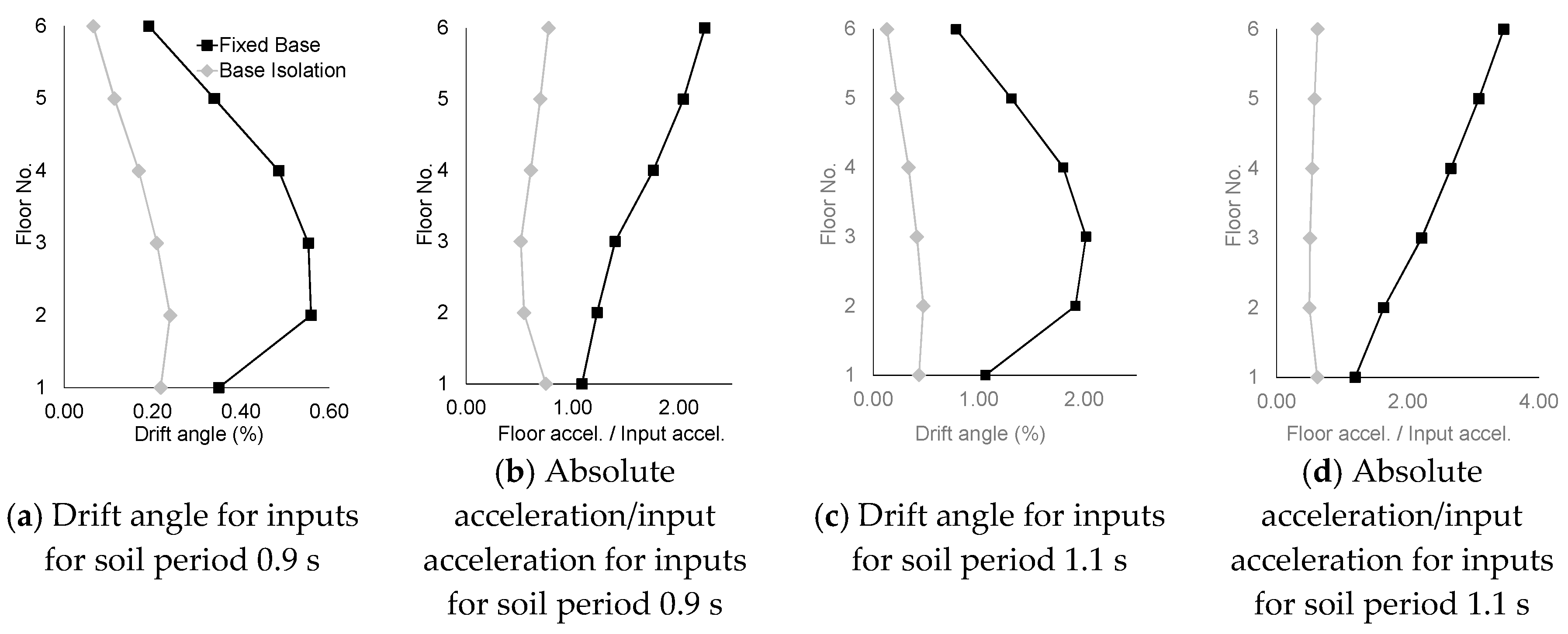
From the information in Table 8 and Table 9, Figure 6 depicts, for further clarity, vertical profiles of drift angles (Figure 6a,c) and normalized absolute accelerations (Figure 6b,d). The results in Figure 6 correspond to the “x + y” cases.

Table 10. Maximum and cumulated response values for the selected inputs.

Input			Maximum * Drift Angle (%)		Maximum * Shear Force/Supported Weight		Maximum * Accel./Input Acceleration		Eζ/EI (Struct. Damp.)	EHD/EI (Dampers)	EHI/EI (Isolators)
Code	Period (s)	Direction	Fixed-Base	Base Isolation	Fixed-Base	Base Isolation	Fixed-Base	Base Isolation	Base Isolation
NR0.9-3	0.9	x	0.388	0.108	0.151	0.042	2.79	0.771	0.196	0.551	0.247
		y	0.293	0.169	0.099	0.057	1.707	0.886	0.176	0.507	0.312
		x + y	0.400	0.168	0.156	0.058	2.281	0.723	0.177	0.508	0.313
NR0.9-6	0.9	x	0.363	0.108	0.148	0.044	2.493	0.716	0.151	0.557	0.292
		y	0.416	0.137	0.133	0.049	2.457	0.799	0.165	0.509	0.326
		x + y	0.388	0.151	0.164	0.061	2.394	0.812	0.148	0.525	0.327
AW0.9-1	0.9	x	0.271	0.113	0.101	0.041	1.996	0.799	0.165	0.565	0.262
		y	0.296	0.157	0.114	0.050	1.813	0.809	0.192	0.519	0.285
		x + y	0.421	0.184	0.148	0.059	2.052	0.788	0.167	0.552	0.276
NR1.1-5	1.1	x	0.689	0.191	0.317	0.083	2.531	0.656	0.145	0.532	0.322
		y	1.299	0.308	0.391	0.104	3.422	0.66	0.156	0.491	0.351
		x + y	1.460	0.294	0.410	0.117	3.652	0.665	0.151	0.532	0.316
NR1.1-7	1.1	x	1.028	0.265	0.444	0.123	3.212	0.628	0.154	0.531	0.314
		y	1.451	0.359	0.432	0.131	4.032	0.740	0.190	0.489	0.315
		x + y	1.632	0.332	0.444	0.154	4.166	0.782	0.176	0.527	0.297
AW1.1-1	1.1	x	0.716	0.174	0.301	0.079	2.457	0.528	0.138	0.533	0.328
		y	0.980	0.359	0.294	0.080	2.843	0.492	0.144	0.488	0.366
		x + y	1.280	0.282	0.410	0.106	2.571	0.428	0.137	0.519	0.342

* “Maximum” refers to both the building height and the input duration.

displays the maximum drift angle, shear force and absolute acceleration for each input in Table 8 and Table 9. The maxima in Table 10 refer to both the building height (1st to 6th stories) and the shaking duration. As in Table 8 and Table 9, the shear force and absolute acceleration are normalized with respect to the supported weight and the maximum input acceleration, respectively. Again, as in Table 8 and Table 9, the results for fixed-base conditions are obtained by supposing that the structure behaves linearly and, thus, are included only for comparison. For the base-isolated building, Table 10 displays also the ratios between the absorbed energies (E_ζ, E_HD, E_HI) and the input energy E_I. E_ζ, E_HD and E_HI are the energy dissipated by the structural damping, the viscous dampers and the rubber bearings, respectively; at the end of the shake, the energy balance reads E_I ≈ E_ζ + E_HD + E_HI.

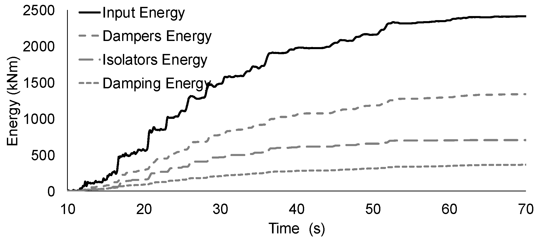
To analyze the time evolution of the energy balance, Figure 7 represents the time-histories of the energies E_I, E_ζ, E_HD and E_HI (Table 10) for the input NR0.9-6 (Table 6); “Input Energy”, “Damping Energy”, “Dampers Energy” and “Isolators Energy” account for E_I, E_ζ, E_HD and E_HI, respectively.

Table 8, Table 9 and Table 10, and Figure 6 and Figure 7 provide the following remarks:

▪

Drift angle in the superstructure. Except in few cases, the isolation reduces the drift displacements; for the 0.22 g inputs (Table 9), that lessening is higher in the top stories. In base isolation conditions, the drift is rather moderate, even for the strongest inputs (Table 9); this trend confirms that the assumption of linear behavior for the superstructure is correct. Finally, comparison between the results for inputs with maximum acceleration 0.1 g and 0.22 g shows that the reduction generated by the isolation is greater for the strongest inputs; this difference can be explained by the non-linear behavior of the lead-rubber bearings: the higher the shear strain, the higher the equivalent damping and the lower the effective secant stiffness, thus leading to a more intense isolation.

▪

Drift angle in the isolators. The shear strains for the inputs with acceleration 0.22 g (Table 9) are more than 2.2 times higher than those for the inputs with 0.1 g (Table 8). Obviously, this circumstance implies non-linear behavior of the lead-rubber bearings. On the other hand, no relevant permanent displacements are observed; this can be read as a satisfactory behavior of the isolation units.

▪

Shear coefficient in the superstructure. The isolation diminishes significantly the story shear forces; that decreasing is higher for the top stories and the strongest inputs. For the base-isolated building, the shear coefficient is near-constant along the building height; this seems to indicate a high participation of the first mode.

▪

Base shear coefficient. As expected, the isolation reduces appreciably the base shear force. For the less severe inputs (0.1 g, Table 8), the diminution ranges between 55% (“y” case) and 70% (“x” case); for the strongest inputs (0.22 g, Table 9), the lessening is roughly 75% in all the cases. This difference can be explained by the non-linear behavior of the lead-rubber bearings.

▪

Absolute acceleration in the superstructure. The absolute acceleration at the ground floor (above the isolation layer) is not reduced, compared to the driving input; in numerous cases, it is even slightly increased. This undesired circumstance might be due to the soft soil influence. However, in the other floors, the absolute acceleration is decreased, compared to the fixed-base case; more precisely, as is common in seismically isolated buildings, the reduction is higher in the top stories. As well, such decreasing is more important for the inputs with acceleration 0.22 g (Table 9). It is well known that the spectral ordinate is roughly equivalent to the ratio between the ground and the top floor acceleration; accordingly, the percentages of reduction of the top floor absolute acceleration and the base shear force are rather similar.

▪

Dissipated energy. Table 10 shows that the percentage of energy dissipated at the isolation interface (E_HD + E_HI, corresponding to viscous dampers and lead-rubber bearings, respectively) is above 80% of the input energy, being slightly higher for the stronger inputs (Table 9). Comparison with the ordinary values of the ratio between the input and hysteretic energies [45] shows that this percentage is clearly above the common demands in terms of energy contributable to damage. Plots from Figure 7 show that the maximum values are obtained at the end of shake; this observation confirms that, for energy-based design, using the final values of energy is an adequate strategy.

▪

Simultaneity of the x and y inputs. As expected, for both the fixed-base and base-isolated buildings, the average drift ratios and shear coefficients for the simultaneous action of the x and y inputs are bigger than those generated by the x and y inputs acting separately. Conversely, regarding the absolute acceleration, the balance is unclear; this apparent inconsistency can be explained by the small building asymmetry (Section 2.1), as any unidirectional input can generate responses containing x, y and torsion (φ) components (Table 4). Broadly speaking, the strategy of combining the full value in one direction with 30% of the value in the orthogonal direction seems to be sufficiently conservative.

6.3. Results for the Rubber Bearings

Apart from the general considerations in Section 6.2, this subsection discusses the performance of the rubber bearings in terms of buckling instability and shear deformation.

Table 11. Maximum * response values for the bearings No. 29 (NRB **), 32 (LRB ***), 24 (LRB **) and 17 (LRB **).

Input			Axial Force (kN)				Torsion Angle (rad)	Drift Displacement (mm)
Code	Period (s)	Input Direction	No. 32	No. 24	No. 29	No. 17
NR0.9-3	0.9	x	338.1	266.5	12.7	409	0.00129	44
		y	467.8	921.5	430.3	789.1	0.00176	104
		Combination	577.2	1001.5	434.1	911.8	0.00180	105
		x + y	645.5	1010.9	424.7	713.9	0.00175	103
NR0.9-6	0.9	x	361.2	284.4	13.8	408.2	0.00129	46
		y	370.2	738	342.3	630.7	0.00143	76
		Combination	517.2	823.3	346.4	753.2	0.00143	77
		x + y	681.8	935.1	294.6	527.3	0.00127	89
AW0.9-1	0.9	x	398.6	315.7	10.5	343.9	0.00136	42
		y	246.5	484.8	226.9	415	0.00164	76
		Combination	472.6	579.5	230.1	539.0	0.00164	77
		x + y	298.4	397.5	218.3	567.1	0.00161	86
NR1.1-5	1.1	x	594	466.9	22.3	717.4	0.00229	186
		y	839.7	1669.2	772.3	1435.4	0.00321	255
		Combination	1028.6	1809.3	779.0	1650.6	0.00320	261
		x + y	1188.6	1849.8	695.9	1367.8	0.00290	272
NR1.1-7	1.1	x	712.7	564.7	24.4	959.2	0.00317	329
		y	967.5	1938.1	882.6	1661.5	0.00375	355
		Combination	1201.7	2107.5	889.9	1949.3	0.00375	369
		x + y	1013.6	1971.3	918.5	2368.8	0.00391	491
AW1.1-1	1.1	x	606.9	477.3	15.6	543	0.00208	163
		y	499.7	990.7	458.5	849	0.00258	182
		Combination	786.1	1133.9	463.2	1011.9	0.00258	189
		x + y	624	1052	449.2	1309.5	0.00237	247
D + 0.5 L	-	-	2755.4	2565	4349	3730	-	-

* “Maximum” refers to the input duration. **/*** 800/700 mm diameter.

shows, for the isolators Nos. 29, 32, 24 and 17 (Figure 2), the maximum values of axial force, torsion angle and drift displacement. The displayed results correspond to the seismic inputs in Table 10; the axial force generated by the gravity loads (combination D + 0.5 L) is also shown (bottom row). In a similar way to Table 8 through Table 10, results for “x”, “y” and “x + y” inputs are presented; herein, results corresponding to the combination of the responses in “x” and “y” directions are also shown. These combinations are obtained according to the European regulations [19]; two empirical criteria are considered: SRSS (square root of sum of squares), and X + 0.3Y or Y + 0.3X. X and Y represent the effect of the inputs in x and y directions, respectively. For the axial force and torsion angle, the combinations are $\sqrt{X^2+Y^2}$, on one hand, and X + 0.3Y or Y + 0.3X, on the other hand; for the drift displacements, the combinations are $\sqrt{X^2+{\left(0.3Y\right)}^2}$ and $\sqrt{{\left(0.3X\right)}^2+Y^2}$. Comparison among the cases “Combination” and “x + y”, shows low correlation; in some cases, the simplified values for “Combination” are over-conservative while in other cases they are extremely under-conservative. This shows that the usual empirical combination criteria are not always on the safe side.

The results in Table 11 are used next to check, in terms of buckling instability and maximum shear strain, the requirements of the Chinese code [12] and the European regulation [20] (8.2.3.4).

Buckling stability. The Chinese code [12] indicates that the average drift displacement in the rubber isolators should not exceed 0.55 times the rubber diameter. This condition is fulfilled in almost all the cases; more precisely, that threshold is only (slightly) exceeded in one case (corresponding to a “x + y” case). The Chinese code does not explicitly require consideration of that coincident actuation; for this unclear situation, the European regulation [21] is considered instead. In that code, it is required that the demanding axial force does not exceed the critical load of each isolator unit; such force is given by P_cr = λ G A_r a′ S/T_q, where λ = 1.1 (for circular devices), G is the rubber shear deformation modulus, A_r is the rubber bearing plan area, a′ is the device diameter, S is the shape factor (ratio between the diameter of the device and the thickness of each rubber layer) and T_q is the total rubber thickness. By neglecting (conservatively) the stiffening effect of the lead plug, the following two values of the critical load are obtained:

$$\begin{array}{c}700\mathrm{mm}\mathrm{diameter}{P}_{\mathrm{cr}}=2.10\times {10}^4 \mathrm{kN}\\ 800\mathrm{mm}\mathrm{diameter}{P}_{\mathrm{cr}}=2.80\times {10}^4 \mathrm{kN}\end{array}$$

Table 11 shows that the maximum axial forces in the 700 and 800 mm isolators are N_Ed,max = 4536 kN (device No. 24, input NR1.1-7, case “x + y”) and N_Ed,max = 6099 kN (device No. 17, input NR1.1-7, case “x + y”), respectively; thus, in both cases N_Ed,max < P_cr/4. On the other hand, [21] prescribes that it should be also checked that δ ≤ 0.7, where δ is the ratio between the design drift displacement d_bd and the device diameter; the design drift is conservatively taken as the maximum value in Table 11: δ = 0.7 and 0.61 for 700 and 800 mm isolators, respectively. Therefore, this criterion is fulfilled in both types of device.

Maximum shear strain. In the European code [21], the maximum design shear strain is given by ε_t,d = ε_c,E + ε_q,max + ε _α,d; in this expression, ε_c,E = 6 S/A_r E′_c, E′_c = 3 G (1 +2 S²), ε_q,max = d_bd/T_q ≤ 2.5, and ε _α,d = 0.003 (a′² + b′²) t_r/2 Σ t³_r, where a′ = b′ (for circular devices), and t_r is the thickness of each rubber layer. For the 700 mm diameter isolators, E′_c = 2882 MPa, and for the 800 mm ones, E′_c = 2614 MPa; then:

$$\begin{array}{c}700\mathrm{mm}\mathrm{diameter}{\mathsf{\epsilon }}_{\mathrm{t},\mathrm{d}}={\mathsf{\epsilon }}_{\mathrm{c},\mathrm{E}}+{\mathsf{\epsilon }}_{\mathrm{q},\max }+{\mathsf{\epsilon }}_{\mathsf{\alpha },\mathrm{d}}=4.77\\ 800\mathrm{mm}\mathrm{diameter}{\mathsf{\epsilon }}_{\mathrm{t},\mathrm{d}}={\mathsf{\epsilon }}_{\mathrm{c},\mathrm{E}}+{\mathsf{\epsilon }}_{\mathrm{q},\max }+{\mathsf{\epsilon }}_{\mathsf{\alpha },\mathrm{d}}=4.90\end{array}$$

Since both above results are smaller than 7/γ_m (where γ_m is a safety factor, being γ_m = 1 in this case), this criterion is fulfilled.

6.4. Influence of Soil–Structure Interaction

To investigate the SSI effect,

Table 12. Maximum * base shear coefficient and rubber shear strain with and without SSI.

Input			Base Shear Force/Building Weight			Shear Strain (%)
Code	Period (s)	Direction	Fixed-Base without SSI	Base Isolation with SSI-a/SSI-b	Base Isolation without SSI	Base Isolation with SSI-a/SSI-b	Base Isolation without SSI
NR0.9-3	0.9	x	0.148	0.041/0.042	0.041	23.40/23.63	22.28
		y	0.097	0.044/0.060	0.056	63.68/58.95	50.18
NR0.9-6	0.9	x	0.145	0.043/0.044	0.043	23.63/23.18	23.18
		y	0.131	0.032/0.048	0.048	37.80/37.78	37.80
AW0.9-1	0.9	x	0.099	0.044/0.042	0.041	22.50/22.50	20.93
		y	0.112	0.035/0.048	0.049	37.35/37.35	37.35
NR1.1-5	1.1	x	0.311	0.085/0.086	0.081	94.28/94.50	92.93
		y	0.384	0.097/0.100	0.102	126.76/126.38	127.53
NR1.1-7	1.1	x	0.436	0.123/0.120	0.121	164.93/164.70	164.25
		y	0.423	0.134/0.126	0.128	177.53/177.53	177.75
AW1.1-1	1.1	x	0.295	0.079/0.081	0.078	83.70/83.70	81.45
		y	0.290	0.072/0.080	0.079	88.43/88.65	90.90

* “Maximum” refers to the input duration.

displays, for the inputs in Table 10, the base shear coefficient in the building (ratio between the base shear force and the building weight), and the shear strain in the rubber bearings (ratio between the isolators drift displacement and the rubber height). Three situations are considered in Table 12: fixed-base without SSI, base isolation with SSI, and base isolation without SSI; like in Table 8 through Table 10, the fixed-base results are determined by assuming linear behavior, and are only displayed for reference. SSI-a and SSI-b have the same meaning than in Table 5. Comparison between the results for base isolation with and without SSI shows that its effect is only moderate, both in terms of base shear and shear strain; therefore, it can be globally concluded that SSI does not play a leading role. The results for both SSI models are rather similar, thus showing little influence of the piles’ vertical stiffness. Comparison between the results for base isolation and fixed-base shows that in all the cases the isolation reduces significantly the base shear; hence, its performance is satisfactory.

6.5. Influence of Changes of the Isolation Units’ Parameters

This section discusses the behavior of the isolation system when the parameters of the isolation units are modified due to heating, rate of loading, scragging, aging, environmental conditions, and manufacturing irregularities. Given the absence of specific prescriptions in the Chinese regulations, the recommendations of [14] are considered. These documents propose a conservative formulation, to be used when no more specific information is available. The major mechanical parameters of the rubber bearings are modified with a factor (λ) that accounts for the aforementioned issues; both maximum and minimum values of λ need to be considered. In NRB, the λ factor affects the stiffness; their maximum and minimum values are 1.83 and 0.77, respectively. In LRB, the λ factor affects the post-yield stiffness and the yielding force; their maximum and minimum values are 1.83/1.84 and 0.77, respectively (1.83 and 1.84 correspond to post-yield stiffness and yielding force, respectively). To analyze the performance of the base isolation under these extreme conditions,

Table 13. Maximum * base shear coefficient and shear strain in the rubber for modified parameters of the isolators.

Input			Base Shear Force/Building Weight		Shear Strain (%)
Code	Period (s)	Direction	Lower Bounds	Upper Bounds	Lower Bounds	Upper Bounds
NR0.9-3	0.9	x	0.037	0.052	23.95	17.01
		y	0.049	0.074	59.81	38.42
NR0.9-6	0.9	x	0.039	0.059	25.41	20.42
		y	0.043	0.058	40.47	24.08
AW0.9-1	0.9	x	0.036	0.055	23.07	18.80
		y	0.044	0.065	40.81	28.22
NR1.1-5	1.1	x	0.069	0.114	96.97	71.95
		y	0.078	0.149	117.49	113.48
NR1.1-7	1.1	x	0.109	0.159	188.27	117.88
		y	0.118	0.162	209.78	126.85
AW1.1-1	1.1	x	0.067	0.109	85.76	65.52
		y	0.067	0.108	94.80	73.10

* “Maximum” refers to the input duration.

displays, as in Table 12, the base shear coefficient and the shear strain in the isolation units for the inputs in Table 10. In Table 13, “Lower bounds” and “Upper bounds” refer to the maximum and minimum values of the λ factor, respectively. To understand the results from Table 13, it should be kept in mind that λ > 1 corresponds to stiffer and more resistant devices, while λ < 1 refers to opposite situations.

Results in Table 13 reflect a regular and expected behavior, in which the stiffer and more resistant devices (upper bounds) lead to higher base shear force and lower shear strain (i.e., less intense isolation). Comparison with Table 12 shows that their results (normal condition of the rubber bearings) lie in between those for the lower and upper bounds, and that in all the cases the base isolation reduces significantly the base shear; this last property can be read as a proper performance of the base isolation, even under extreme modifications in the parameters of the rubber bearings. The only exception to the aforementioned regularity is that, for the input NR1.1-5 in the y direction, the shear strain under normal conditions (Table 12) is higher than the corresponding values in Table 13. This circumstance can be explained by the high uncertainties inherent to any non-linear dynamic (time-history) analysis.

7. Conclusions

Aiming to confirm the suitability of seismic isolation in soft soil, this paper presents a numerical analysis on the performance of a rubber-isolated 6-story RC teaching building in Shanghai. The verification consists in performing non-linear time-history analyses for a number of seismic inputs that are selected to represent the site seismicity, taking into consideration the soil conditions. Two sets of seven inputs each are considered; in the first and second sets, the inputs are normalized to maximum acceleration of 0.1 g and 0.22 g, respectively. A simplified uncoupled linear model represents the soil–structure interaction. The performance is analyzed even when the mechanical parameters of the isolation units have experienced important changes.

The general conclusion of this study is that, in the analyzed case study, the isolation performs satisfactorily, both in terms of demand on the isolation system and on the superstructure. Specific conclusions are discussed next.

▪

Global. Isolation reduces significantly the base shear force, being more efficient for the strongest inputs; also, the SSI effect is rather negligible. Additionally, the simultaneous actuation of both input horizontal components is compared with the usual simplified combination criteria; it is concluded that they frequently underestimate the demand.

▪

Isolation layer. The demand on the isolators is checked in terms of buckling instability and shear strain; on the other hand, the percentage of hysteretic energy that is dissipated by the isolation interface is high, clearly above common demands. Finally, it is observed that there are no relevant permanent displacements.

▪

Superstructure. Relative displacements, shear forces and absolute accelerations are significantly reduced, except the ground floor accelerations.

This research seems to point out that base isolation, if properly designed and implemented, can be an efficient solution for ordinary mid-height RC buildings founded on soft soil and located in medium seismicity regions, like Shanghai. This conclusion may support the promotion of seismic isolation in soft soils; notably, these terrains are particularly frequent in numerous densely populated urban areas.

References

1. Kelly, J.M. Aseismic base isolation: Review and bibliography. Soil Dyn. Earthq. Eng. 1986, 5, 202–217. [Google Scholar] [CrossRef]
2. Buckle, I.G.; Mayes, R.L. Seismic isolation: History, application, and performance. A world overview. Earthq. Spectra 1990, 6, 161–202. [Google Scholar] [CrossRef]
3. Koh, H.M.; Song, J.; Ha, D.H. Cost effectiveness of seismic isolation for bridges in low and moderate seismic region. In Proceedings of the 12th World Conference on Earthquake Engineering (12WCEE), Auckland, New Zealand, 30 January–4 February 2000; p. 1100. [Google Scholar]
4. Deb, S.K. Seismic base isolation—An overview. Curr. Sci. 2004, 87, 1426–1430. [Google Scholar]
5. Higashino, M.; Okamoto, S. (Eds.) Response Control and Seismic Isolation of Buildings; Taylor & Francis: Milton Park, UK, 2006. [Google Scholar]
6. Constantinou, M.; Kneifati, M. Dynamics of Soil-Base-Isolated-Structure Systems. J. Struct. Eng. ASCE 1988, 114, 211–221. [Google Scholar] [CrossRef]
7. Vlassis, A.G.; Spyrakos, C.C. Seismically isolated bridge piers on shallow stratum with soil–structure interaction. Comput. Struct. 2001, 79, 2847–2861. [Google Scholar] [CrossRef]
8. Spyrakos, C.C.; Koutromanos, I.A.; Maniatakis, C.A. Seismic response of base-isolated buildings including soil–structure interaction. Soil Dyn. Earthq. Eng. 2009, 29, 658–668. [Google Scholar] [CrossRef]
9. Spyrakos, C.C.; Maniatakis, C.A.; Koutromanos, I.A. Soil-structure interaction effects on base-isolated buildings founded on soil stratum. Eng. Struct. 2009, 31, 729–737. [Google Scholar] [CrossRef]
10. Enomoto, T.; Yamamoto, T.; Ninomiya, M.; Miyamoto, Y.; Navarro, M. Seismic Response Analysis of Base Isolated RC Building Building Considering Dynamical Interaction Between Soil and Structure. In Proceedings of the 15th World Conference on Earthquake Engineering (15WCEE), Lisbon, Portugal, 24–28 September 2012; p. 3611. [Google Scholar]
11. Alavi, E.; Alidoost, M. Soil-Structure Interaction Effects on Seismic Behavior of Base-Isolated Buildings. In Proceedings of the 15th World Conference on Earthquake Engineering (15WCEE), Lisbon, Portugal, 24–28 September 2012; p. 4982. [Google Scholar]
12. GB50011. Code for Seismic Design of Buildings; Ministry of Housing and Urban-Rural Development: Beijing, China, 2010. [Google Scholar]
13. E.030. Norma Técnica de Edificación E.030 Diseño Sismorresistente; Ministerio de Vivienda, Construcción y Saneamiento: Madrid, Spain, 2014. [Google Scholar]
14. ASCE 7–16. Minimum Design Loads and Associated Criteria for Buildings and Other Structures; American Society of Civil Engineers: Reston, VA, USA, 2016. [Google Scholar]
15. Zhou, Y.; Wu, C.X.; Zhang, C.L. Analysis and Design of Seismic Isolation Structure in Outpatient Building of the Lushan County People’s Hospital. Build. Struct. 2013, 43, 23–27. (In Chinese) [Google Scholar]
16. Weng, D.; Zhang, S.; Hu, X.; Chen, T.; Zhou, Y. Seismic Isolation Design Soil of a Teaching Building for Shanghai Foreign Language School; Research Institute of Structural Engineering and Disaster Reduction, Tongji University: Shanghai, China, 2012. (In Chinese) [Google Scholar]
17. Weng, D.; Tao, L.; Alfarah, B.; López-Almansa, F. Nonlinear time-history analysis of a base-isolated RC building in Shanghai founded on soft soil. In Proceedings of the 16th World Conference on Earthquake Engineering (16WCEE), Santiago de Chile, Chile, 9–13 January 2017; p. 2634. [Google Scholar]
18. CSI Analysis Reference Manual for SAP2000®, ETABS®, and SAFE®; CSI (Computers and Structures, Inc.): Berkeley, CA, USA, 2010.
19. EN 1998-1. Eurocode 8: Design of Structures for Earthquake Resistance; European Committee for Standardization: Brussels, Belgium, 2004. [Google Scholar]
20. EN 15129. Anti-Seismic Devices; European Committee for Standardization: Brussels, Belgium, 2009. [Google Scholar]
21. EN 1337-3. Structural Bearings. Part 3: Elastomeric Bearings; European Committee for Standardization: Brussels, Belgium, 2005. [Google Scholar]
22. GB50009. Load Code for Design of Building Structures; Ministry of Housing and Urban-Rural Development: Beijing, China, 2010. [Google Scholar]
23. Inaudi, J.A.; Kelly, J.M. Optimum damping in linear isolation systems. Earthq. Eng. Struct. Dyn. 1993, 22, 583–598. [Google Scholar] [CrossRef]
24. DGJ 08-37. Code for Investigation of Geotechnical Engineering; Shanghai Geotechnical Investigations & Design Institute Co, Ltd.: Shanghai, China, 2012. [Google Scholar]
25. FEMA 356. Prestandard and Commentary for the Seismic Rehabilitation of Buildings; Federal Emergency Management Agency: Washington, DC, USA, 2000. [Google Scholar]
26. Castaldo, P.; De Iuliis, M. Optimal integrated seismic design of structural and viscoelastic bracing-damper systems. Earthq. Eng. Struct. Dyn. 2014, 43, 1809–1827. [Google Scholar] [CrossRef]
27. Ou, J.P.; Long, X.; Li, Q.S. Seismic response analysis of structures with velocity-dependent dampers. J. Constr. Steel Res. 2007, 63, 628–638. [Google Scholar] [CrossRef]
28. Luco, J.E. Effects of soil–structure interaction on seismic base isolation. Soil Dyn. Earthq. Eng. 2014, 66, 167–177. [Google Scholar] [CrossRef]
29. Hatami, F.; Nademi, H.; Rahaie, M. Effects of Soil-Structure Interaction on the Seismic Response of Base Isolated in High-Rise Buildings. Int. J. Struct. Civ. Eng. Res. 2015, 4, 237–242. [Google Scholar] [CrossRef] [Green Version]
30. Sayyad, S.T.; Bhusare, V. Effectiveness of base isolator in high-rise building for different soil conditions using FEM. Int. J. Sci. Dev. Res. 2016, 1, 291–295. [Google Scholar]
31. FEMA 273. NEHRP Guidelines for the Seismic Rehabilitation of Buildings; Federal Emergency Management Agency: Washington, DC, USA, 1997. [Google Scholar]
32. Gazetas, G.; Makris, N. Dynamic pile-soil-pile interaction. Part I: Analysis of axial vibration. J. Earthq. Eng. Struct. Dyn. 1991, 20, 115–132. [Google Scholar] [CrossRef]
33. ATC-40. Seismic Evaluation and Retrofit of Concrete Buildings; Applied Technology Council: Redwood City, CA, USA, 1996. [Google Scholar]
34. Gazetas, G. Formulas and charts for impedances of surface and embedded foundations. J. Geotech. Eng. ASCE 1991, 117, 1363–1381. [Google Scholar] [CrossRef]
35. UBC (Uniform Building Code); International Council of Building Officials: Lansing, MI, USA, 1997.
36. PKPM. SATWE Users’ Manual. 2014. Available online: http://www.pkpm.cn/ (accessed on 12 December 2020).
37. DGJ 08-9. Code for Seismic Design of Buildings; Tongji University Shanghai Urban Construction and Communication Commission: Shanghai, China, 2013. [Google Scholar]
38. PEER. Users Manual for the PEER Ground Motion Database Web Application; Technical Report; Pacific Earthquake Engineering Research Center (PEER): Berkeley, CA, USA, 2011. [Google Scholar]
39. Arias, A. A Measure of Earthquake Intensity. Seismic Design for Nuclear Power Plants; MIT Press: Cambridge, MA, USA, 1970; pp. 438–443. [Google Scholar]
40. Manfredi, G. Evaluation of seismic energy demand. Earthq. Eng. Struct. Dyn. 2001, 30, 485–499. [Google Scholar] [CrossRef]
41. Trifunac, M.D.; Brady, A.G. Study on the duration of strong earthquake ground motion. Bull. Seismol. Soc. Am. 1975, 65, 581–626. [Google Scholar]
42. Gomase, O.; Bakre, S. Performance of Non-Linear Elastomeric Base-Isolated building structure. Int. J. Civ. Struct. Eng. 2011, 2, 280–291. [Google Scholar]
43. Castaldo, P.; Gino, D.; Mancini, G. Safety formats for non-linear finite element analysis of reinforced concrete structures: Discussion, comparison and proposals. Eng. Struct. 2019, 193, 136–153. [Google Scholar] [CrossRef]
44. Haukaas, T.; Gardoni, P. Model uncertainty in finite-element analysis: Bayesian finite elements. J. Eng. Mech. 2011, 137, 519–526. [Google Scholar] [CrossRef]
45. López Almansa, F.; Yazgan, U.; Benavent Climent, A. Design energy input spectra for moderate-to-high seismicity regions based on Turkish registers. Bull. Earthq. Eng. 2013, 11, 885–912. [Google Scholar] [CrossRef] [Green Version]
Figure 1. Analyzed case study building.
Buildings 10 00241 g001
Figure 2. Installation of isolators and dampers in the building.
Buildings 10 00241 g002aBuildings 10 00241 g002b
Figure 3. Spatial (3-D) model of the building structure.
Buildings 10 00241 g003
Figure 4. Comparison between the response spectra of the natural selected inputs and the code design spectra.
Buildings 10 00241 g004
Figure 5. Dynamic responses of two isolators and a damper for input NR1.1-7 in the x direction (Table 7).
Buildings 10 00241 g005
Figure 6. Vertical profiles of drift angles and absolute accelerations for combined x + y inputs.
Buildings 10 00241 g006
Figure 7. Time-history of the energy components for the input NR0.9-6 (Table 6).
Buildings 10 00241 g007