Article

Improving the Accuracy of a Hygrothermal Model for Wood-Frame Walls: A Cold-Climate Study

by
Charles R. Boardman
* and
Samuel V. Glass
Building and Fire Sciences, US Forest Service Forest Products Laboratory, Madison, WI 53726, USA
*
Author to whom correspondence should be addressed.
Buildings 2020, 10(12), 236; https://doi.org/10.3390/buildings10120236
Submission received: 15 November 2020 / Revised: 3 December 2020 / Accepted: 4 December 2020 / Published: 11 December 2020
(This article belongs to the Section Building Materials, and Repair & Renovation)

Abstract

:
A one-dimensional transient hygrothermal model was used to simulate eight different wood-frame wall assemblies. Simulations were compared with measured results from a two-year field study exploring the effects of exterior insulation on wall moisture performance in a cold-climate. The field study documented the moisture content, temperature, and relative humidity measurements in wall assemblies using oriented strand board (OSB) sheathing. Simulations were performed using generic design input values as well as input values based on measurements or sensitivity analysis. Laboratory material property measurements informed the choice of material property values in the improved model for OSB, asphalt-coated kraft paper, and interior latex paint. Simulations using improved input values typically agreed with field measurements within measurement error. The most significant model improvements were all related to vapor permeance. The vinyl siding used an effective permeance much lower than typically recommended. However, both the extruded polystyrene insulation and the asphalt-coated kraft paper facing on the cavity fiberglass insulation had higher permeance than literature values.

1. Introduction

There is continued interest in increasing the energy efficiency of buildings in North America, much of which is driven through green building standards and code changes such as in the International Energy Conservation Code (IECC). A recent U.S. Department of Energy analysis indicated that adoption of the 2018 IECC would reduce energy costs compared to the 2015 code [1], while earlier code changes produced a 32% cost saving between 2006 and 2012 [2]. Design of energy efficient buildings requires careful consideration of moisture, in addition to energy, to ensure durability [3]. The Forest Products Laboratory has undertaken a joint project with APA—The Engineered Wood Association to evaluate the effects of insulation applied outside the sheathing on the durability of wood-framed structures [4]. A detailed research report documents the instrumentation and monitoring results for a wood-framed test hut using split-insulation with a variety of exterior insulations placed over Oriented Strand Board (OSB) in the cold-climate of Madison, WI, USA [5]. As part of that project, this report documents details of the hygrothermal modeling for that wood-framed structure. The model can be used to predict moisture performance of similar wall structures in different climates, thus helping to evaluate the overall durability of these wall designs.
WUFI [6] is a hygrothermal simulation tool commonly used both for building design and research. We used WUFI Pro 6.4, the one-dimensional version of this family of software products which calculate transient coupled heat and moisture transport, to model the test wall assemblies. This tool has been used widely in North America for simulation of wood-frame walls [7,8,9,10,11,12]. WUFI Pro software simulation methods have been extensively validated [13]. For example, early work in Sweden highlighted the importance of air flow in the gap between exterior insulation and the cladding but found good agreement between calculated and measured values given the correct boundary conditions [14]. A more extensive validation using data from five Swedish homes, but coming to the same conclusions, was summarized in work by Mundt-Petersen and Harderup [15]. However, a validated model is just the first step in using a simulation tool for building design and research. Lstiburek et al. [16] provide guidelines for less-experienced practitioners so they can avoid unrealistic results. In this work we draw from the example of Lstiburek et al. for modeling enclosure design [17]. Other relevant resources to inform WUFI modeling practice include Fox’s thesis [18] and Trainor’s work [19] on High-R wall assemblies. Practical advice in a blog for working designers, along with helpful commentary, illustrate the state of the art in 2018 [20].
The primary objective of this work was to demonstrate that WUFI model output can match measured values of OSB moisture content (MC), cavity temperature (T), and cavity relative humidity (RH) within the limits of measurement error for wood-framed walls with a variety of exterior insulations in a cold climate. Secondary objectives were to illustrate the effects of select material properties and real boundary conditions (indoor and outdoor temperature and relative humidity, along with solar radiation, local wind speed and direction, and rain) on model predictions, and to explore the sensitivity of the model to a variety of modeling choices. This report first reviews the experimental results against which the model is compared. Next, design values, which could be obtained without reference to measured data, are chosen to set the framework for analysis of the 8 different wall sections of the test hut. Then, based on insight gained from comparing model predictions to measured values and from the laboratory material property measurements, improvements to the model are outlined and justified. The improved model is compared both with the design model and measured data for all wall configurations. Selected sensitivity studies are presented to illustrate the effects of key modeling choices and material properties. Finally, we provide a summary of the significant properties in the improved model. We were surprised to find that the vinyl siding needed an effective vapor permeance much lower than typically recommended. However, both the extruded polystyrene insulation and the asphalt-coated kraft paper facing on the cavity fiberglass insulation required higher vapor permeance than literature values. The results of this work and example model contribute to the validation of WUFI Pro and the education of design practitioners and researchers. Improved building modeling supports the creation of more durable energy-efficient buildings.

2. Measurements

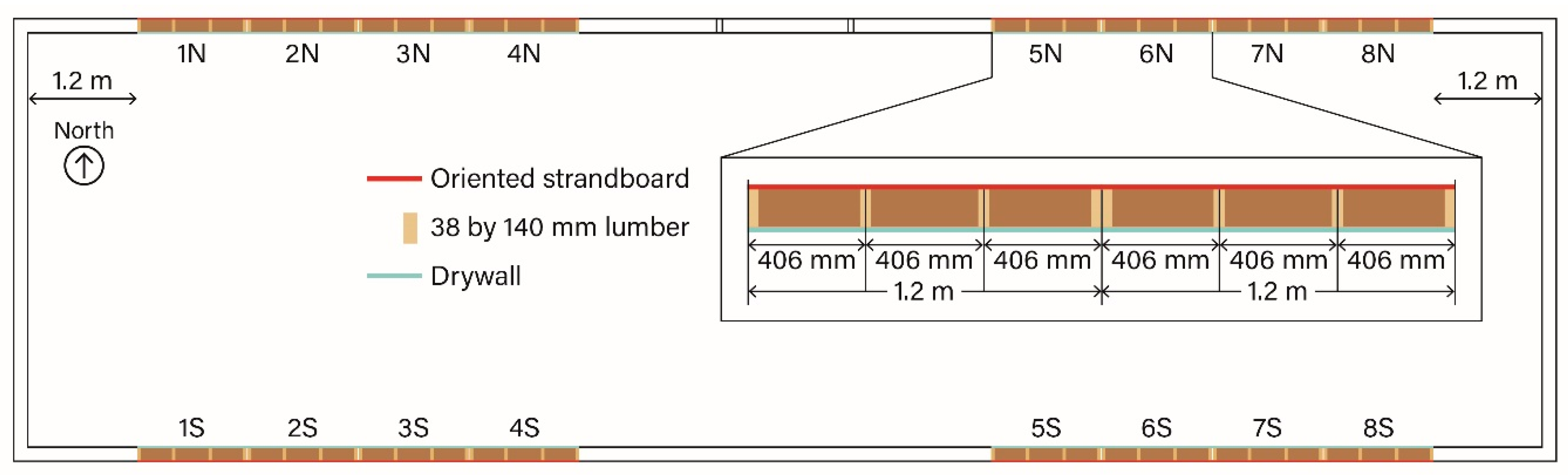
2.1. Overview of Field Measurements

The test structure, built with 38 by 140 mm (nominal 2″ × 6″) wood framing, contained 16 test bays, with eight different configurations, one facing North and an identical one facing South. See Figure 1 for an overview and [5] for full details. All wall assemblies included vinyl siding, spun-bonded polyolefin house wrap, oriented strand board (OSB) sheathing, fiberglass batt cavity insulation (3.7 m2·K/W or R-21), and painted interior gypsum drywall.
The various configurations are detailed in Table 1. The variation in assembly across the 8 configurations reflected different kinds of exterior insulation (or none), different interior vapor retarders, and different application of the water-resistive barrier (WRB). All cavities, except wall 8, had flat spun-bonded polyolefin WRB. Wall 8 used a drain wrap with a crinkled surface made from polyolefin. There were only two variations in the interior vapor retarder. One was the kraft-facing of the fiberglass batt and the other was a polyethylene sheet (poly). The final variations included three kinds of insulation outboard of the OSB: expanded polystyrene (EPS—38 mm), extruded polystyrene (XPS—25.4 mm), and mineral wool (MW—38 mm).
Each cavity had a probe attached to the inside surface of the OSB, providing a relative humidity (RH, ±5%) and temperature (T, ±1.2 °C) reading in the cavity 5 mm from the OSB surface and near the top of the cavity, see Figure 2.
Each cavity was wetted with 40 g of water per day for three to five days three times during the two-year data collection period. That water was deposited on a paper towel fixed to the inner OSB surface to allow wetting the OSB and evaporation into the cavity. Each cavity also had 4 moisture pin pairs to read OSB moisture content (MC, ±1.3%), two of which were in the field of the paper towel and two of which were outside that field. These are the field measurements which are compared to model predictions below.

2.2. Material Property Measurements

Select material properties were measured in the laboratory to inform the modeling and check literature values for key wall components. Samples of OSB, kraft paper, and gypsum wallboard with paint, were used for water vapor transmission tests (wet and dry cup) according to ASTM standard E96-16 [21]. The water vapor permeance for all tested materials is summarized in Table 2.
Sixteen OSB specimens (near 0.2 m × 0.2 m square and 11 mm thick) were cut for water vapor transmission measurements, 8 for wet cup and 8 for dry cup. The wet cup measurements were made with deionized water in the cup, and the dry cup measurements were made with molecular sieve desiccant in the cup. All cups were placed in a room maintained near 50% RH and 23 °C. Each cup was weighed on an electronic balance with resolution of 0.01 g each day until the slope of mass versus time was constant (over 1 month). Another wet cup was sealed on top with metal, rather than OSB, to measure leakage of the cup system. Analysis proceeded according to the standard, taking account of masked edge effects, surface resistances, and still air resistance.
Ten specimens of kraft paper backing were removed from the fiberglass insulation and cut to size (near 0.2 × 0.2 m square and 0.14 mm thick). Five were used for the wet cup and five for the dry cup, just like the OSB samples except it took less than a month for the mass change rates to stabilize. Dry cup values (Table 2) were considerably higher than the maximum value of 57 ng/Pa s m2 (1 US perm) for a Class II vapor retarder. While the dry cup values were within the range reported in the literature, the wet cup average permeance was higher than the literature values. This may be a result of variation in the manufacturing process of asphalt-coated kraft paper, but the sampling in this study was too small to draw any conclusion. Further investigation is warranted but outside the scope of this paper.
Four specimens of gypsum drywall with paint were cut from test walls after completion of the field study (near 0.17 × 0.17 m and 12.7 mm thick) for water vapor transmission measurements. The humidity and temperature conditions were different from standard conditions: the mean RH values were 51% RH (23.9 °C) in the two wet cup experiments and 31% RH (22.3 °C) in the two dry cup experiments. These two average conditions were chosen to bracket extremes of indoor relative humidity in the test hut during winter and spring. Humidity chambers were used to control the conditions outside the test cups to achieve these average conditions. For the wet cup experiment the humidity chamber was set to 27% RH, while a saturated sodium chloride solution was used inside the wet cup (75% RH). For the dry cup experiment the humidity chamber was set to 62% RH, while the molecular sieve desiccant was used inside the dry cup. It took only a few days to achieve a steady mass change rate.

3. Hygrothermal Model: Initial Design Values

When hygrothermal simulations are used for design analysis, actual material properties may not be known with precision, and practitioners rely on property values from the literature or databases within the simulation software. In this section we use this approach to provide a baseline for comparison. Wall assemblies were modeled with WUFI Pro software, version 6.4 [6]. WUFI modeling did not include the wood framing since it is a one-dimensional model. The other model inputs and outputs are reported in this section. Full details of all material properties are provided in Appendix A, Table A1, Table A2, Table A3, Table A4, Table A5, Table A6, Table A7, Table A8, Table A9, Table A10, Table A11, Table A12, Table A13, Table A14, Table A15, Table A16, Table A17, Table A18, Table A19, Table A20, Table A21, Table A22, Table A23, Table A24, Table A25, Table A26, Table A27 and Table A28.

3.1. Database Material Properties

The material properties for spun-bonded polyolefin, OSB, gypsum drywall, and fiberglass were taken directly from the WUFI Materials database: Spun Bonded Polyolefin Membrane is in the Membranes section of the North American database, with thickness 1 mm; oriented strand board is available in the Building Boards and Sidings section of the North American database, we used the low density (575 kg/m3) version, but with thickness 11.1 mm; Interior Gypsum Board is available in the Building Boards and Siding section of the North American database with 12.5 mm thickness; fiberglass material properties came from the Fiber Glass entry in the Insulation Materials section of the North American database. Wall 8 used drain wrap polyolefin and there is an entry for this called Spun Bonded Polyolefin Membrane with Crinkled Surface in the database. All three of the exterior insulations can be found in the Insulation Materials section of the North American database, as Expanded Polystyrene (38.1 mm), Extruded Polystyrene (25.4 mm), and Rockwool Comfortboard 80 (38.1 mm).
Simple modifications were made to handle the material properties of the vinyl siding. The vinyl siding material base properties came from Lstiburek et al. [17]. Some of those properties are apparently from the Vinyl Wallpaper entry in the Membranes section of the North American database. However, changes from that wallpaper entry included a bulk density of 829 kg/m3 and a thermal conductivity of 0.17 W/m·K. Additional modifications were necessary to reflect the fact that vinyl siding allows air movement through seams and gaps, thus increasing moisture transport in this layer. There are a variety of ways to handle this in modeling, typically using either an effective vapor permeance or an air layer behind the cladding which has an air exchange with the exterior [17,31]. For the design we used a vinyl thickness of 1.11 mm and the effective permeance method by setting the vapor diffusion resistance factor (µ) to 76 (which reflects an effective vapor permeance near 40 US perm). Note that WUFI specifies a material’s water vapor permeance using a dimensionless resistance ratio so the µ-value of 76 indicates the vinyl layer has 76 times the resistance to water vapor movement as still air. This modeling choice for vinyl siding is examined in more detail in the model improvements and sensitivity analysis sections below.
The kraft-facing of the fiberglass batt was modeled as 1 mm thick layer of Kraft Paper from the Membranes (Generic) subsection of the Generic Materials database. The other vapor retarder was a polyethylene sheet modeled as a 1 mm layer of PE-Membrane from the same Generic Materials database. These 1 mm thicknesses are not actual material thickness but the recommended minimum “effective” thickness for membranes to allow at least 5 grid elements of reasonable size in each layer of an assembly. The WUFI default membranes have had their properties adjusted to provide the correct heat and vapor diffusion fluxes.
A wide range of vapor permeance values are reported for latex paint on gypsum. The design value was calculated based on Table 5 (Typical Water Vapor Permeance and Permeability for Common Building Materials) in Chapter 26 (Heat, Air, and Moisture Control in Buildings Assemblies—Material Properties) of the 2017 ASHRAE Handbook of Fundamentals [29] entry for Paint, 3 coats Styrene/butadiene latex coating. That entry shows a dry cup value of 629 ng/Pa s m2 (11 US perm). The translation of this permeance into the model is given below in the wall boundary conditions.

3.2. Boundary Conditions

All walls were set with 90° inclination and used the short building height defaults for driving rain. Each wall was duplicated with both a North and South orientation.
The interior and exterior surface transfer coefficients are important and some of them will be discussed in more detail in the model improvements section below. Default values were used except for the sd value (a water vapor diffusion resistance) of the interior surface. The sd value controls moisture flow by specifying an additional resistance of a surface coating (like paint) based on an equivalent thickness of still air. The exterior surface heat resistance was 0.0588 m2 K/W, with no wind-dependence. There was no sd value, corresponding to the No coating selection for no additional resistance to moisture transfer. Short-wave Radiation Absorptivity, used to account for solar heating from the visible light spectrum, was 0.2 corresponding to the Bright setting. The vinyl siding used in the experiment was white. There was no explicit radiation balance, so the only other radiation setting was that of 0.2 for Ground Short-Wave Reflectivity. The Adhering Fraction of Rain was 0.7. This leaves the setting for any additional moisture transfer resistance on the interior surface, which was set to an sd-value of 0.32 m using the User-Defined selection. This is a value between two of the choices offered by WUFI (Latex paint 1 and 2 in the drop-down menu), to account for the fact that the interior gypsum was painted with a common flat interior latex paint as discussed in the previous section.
The simulation was run for two years. The moisture content of each layer at the end of the simulation for each wall assembly was used to adjust the initial moisture content by manual iteration until there was little difference between starting and ending moisture content. The climate was set to Madison (WI, USA) cold year, and indoor conditions followed the ASHRAE 160 standard [32] with indoor air conditioning and all other values at default. Thus, the heating set point was 21.1 °C with cooling set point at 23.9 °C and no RH control (outside that provided by air conditioning). Indoor moisture generation corresponded to two bedrooms and standard construction indicating 0.2 air changes per hour (ACH) on a building volume of 500 m3. This control method yields large fluctuations in RH throughout the year, with an average RH of 58% in July and 30% in January.

3.3. Numerical Parameters

Each wall assembly was created on a Fine Grid (100 nodes) in WUFI’s Assembly/Monitor Positions under Component. Each simulation was run using both heat and moisture transport calculations with increased accuracy and adapted convergence.

3.4. Results

Figure 3 plots the moisture content (MC) of the OSB for walls without exterior insulation (No CI) and with mineral wool (MW). The simulation starts in winter (28 January) and ends two years later (all weather files start on 1 January, but the simulation starts on 28 January because the measured data, which will be discussed below, became reliable on 28 January). Figure 3a illustrates that north walls (N) have higher predicted MC than south (S), while the right (b) illustrates that the polyethylene vapor barrier keeps the wall drier during winter. Both portions of Figure 3 illustrate that exterior insulation lowers the MC during the winter.
Figure 4 plots the OSB MC for the other north walls with exterior insulation. The crinkled WRB makes no significant difference compared to the plain WRB, while for walls with kraft the MW results in the lowest peak MC and XPS has the highest peak MC. Nevertheless, all insulated walls have lower peak MC than the No CI base case. Further, all of the design walls, including the No Cl base case, were significantly below the 20% MC design limit, indicating no risk of fungal decay [33], and the calculated mold index [32] at the interior OSB surface remains near zero for all walls.

4. Overview of Improvements to the Model

The previous section showed that OSB moisture content stayed below 14% when simulated with design input values. However, field measurements of the wall assembly with interior kraft and without exterior insulation, for example, had OSB moisture content above 25% in winter. It is important to understand which input values have the most impact on simulation results. One important set of inputs is the material properties. In this section we outline and justify property value changes to six materials used in the WUFI design model. Some of these changes, those for vapor permeance of OSB, kraft paper, and the paint layer on the interior gypsum drywall, were based on laboratory measurements (see previous Section 2.2—material property measurements). The rest of the changes, those for the vinyl siding, XPS, and fiberglass, were based on comparison of the model predictions to measured data. These improved values were a result of multiple WUFI runs with a wide variety of parameter changes. Select sensitivity results will be presented later. This section concludes by illustrating how these model improvements affect the design predictions. Then, in the following section, we compare this improved model with measured results using measured boundary conditions.

4.1. Customized Material Properties

4.1.1. Vinyl Siding

As mentioned earlier there are many ways to handle the air flow through vinyl siding. While using an air layer behind the cladding and adding an air exchange with outside air to this layer is a common method to account for these effects, we opted to instead use an effective permeance model. In the sensitivity analysis section, we show that while the extra air layer can work, it may increase model instability. The effective permeance method is robust but there is limited data on what values to use. In the initial model we implemented a design value of 40 US perm [34]. Experimentation with different values and reflection on how these values allowed the model prediction to better match measured values resulted in picking an effective permeance closer to 4 US perm. Specifically, the improved vinyl model used a vapor diffusion resistance factor of 700 (increased from the design value of 76). Further empirical investigation of vinyl siding effective permeance is warranted but outside the scope of this study.
To improve the robustness of the alternative method for accounting for air flow through the vinyl siding an additional change was made to the vinyl properties. Specifically, the water storage function of the vinyl layer was increased by changing the porosity to 1. We illustrate how this increases robustness in the sensitivity analysis section. The vinyl material, like many materials in the WUFI database, did not include any measured water storage, and we would expect very little storage from the actual vinyl material, but the profile of vinyl siding can retain liquid water, primarily by surface adhesion, so there is some physical reason to include water storage in this layer [10]. Further, any material in WUFI, such as this vinyl siding, which does not specifically include a water storage function has a default water storage function applied by WUFI. The amount of water which can be absorbed in this case is controlled by the entry for material porosity. We increased the material porosity from 0.001 to 1 which makes the maximum water storage 47.1 kg/m3 at 100% RH. Changing the porosity does not affect any of the other material properties beyond the moisture storage.
Simulations with different values of the vinyl (exterior surface) short-wave radiation absorptivity showed a significant effect on how well model predictions matched measured values. The improved model reduced this value from 0.2 to 0.07. Details on the effects of this change will be presented in the sensitivity analysis section. Further empirical investigation of vinyl siding radiation absorptivity (both short and long wave) is warranted but outside the scope of this study.

4.1.2. Extruded Polystyrene

We reduced the XPS permeance based on comparison of the model predictions with measured data. The new effective vapor diffusion resistance factor was set to 79 (reduced from the design value of 171), which may reflect air movement between the XPS and WRB which improves drying to the outside.

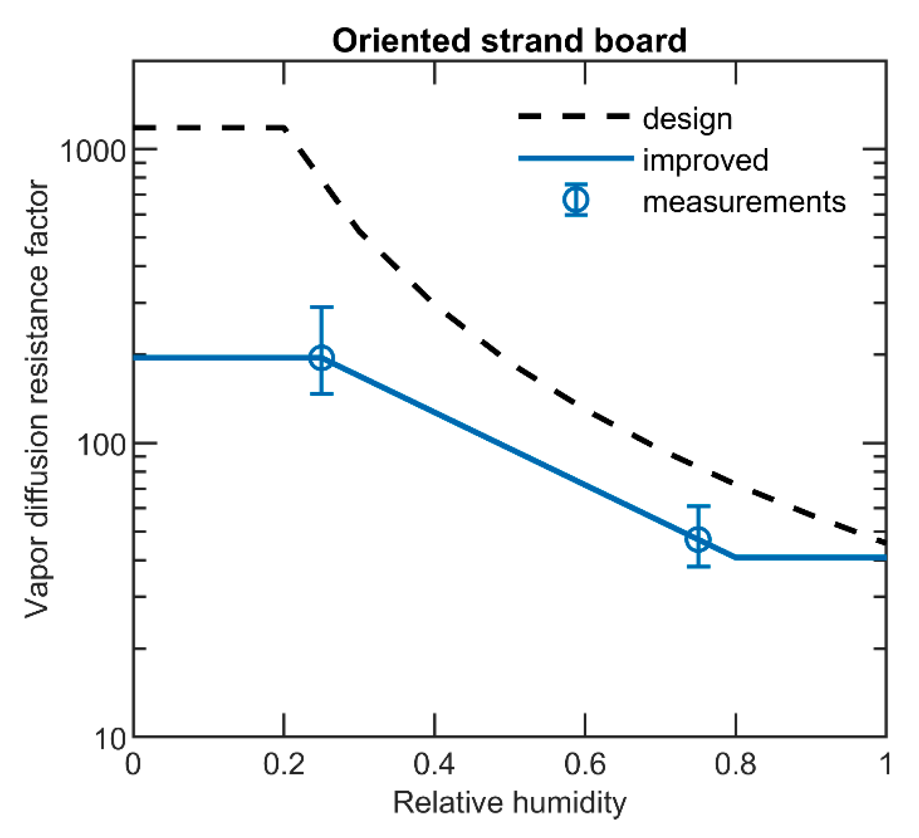
4.1.3. Oriented Strand Board

Literature values for material properties of OSB vary widely. We surveyed part of this literature, with focus on the sorption isotherm, in [35]. The OSB properties used in the improved model are similar to those in an earlier WUFI modeling study [36] reflecting measured values of density, porosity, and vapor permeance. Our OSB had lower density than even the low value used for design, with a slightly reduced thermal conductivity (0.81 W/m K). The density was 534 kg/m3 with porosity 0.64. We set the specific heat capacity to 1280 J/kg K based on the work of Igaz et al. [37]. Most significant was the reduced resistance to vapor diffusion.
Figure 5 plots the measured vapor diffusion resistance factors, at the averages of the dry cup and wet cup RH, along with our improved model and the WUFI standard OSB diffusion resistance curve for the low density OSB in the North American database. Above 80% RH the vapor diffusion resistance factor was held constant because this is the point in the model at which liquid transport begins (to avoid double counting). The default liquid transport coefficients were retained in the improved model.

4.1.4. Fiberglass

Two changes were made to the fiberglass, both based on comparison of the model predictions to measured data in temperature and relative humidity to be explored later. The thermal conductivity was increased from 0.035 to 0.040 W m−1 K−1, reflecting a reduction in resistance probably as a result of less-than-perfect fiberglass batt installation. More significantly the moisture storage was reduced, setting the porosity to 0.008 instead of the default 0.99. This again is based on the default water storage function which WUFI applies to materials without any direct entry. The design fiberglass layer with porosity of 0.99 had an artificially large water storage which affected both the OSB moisture content and the relative humidity measured in the fiberglass layer.

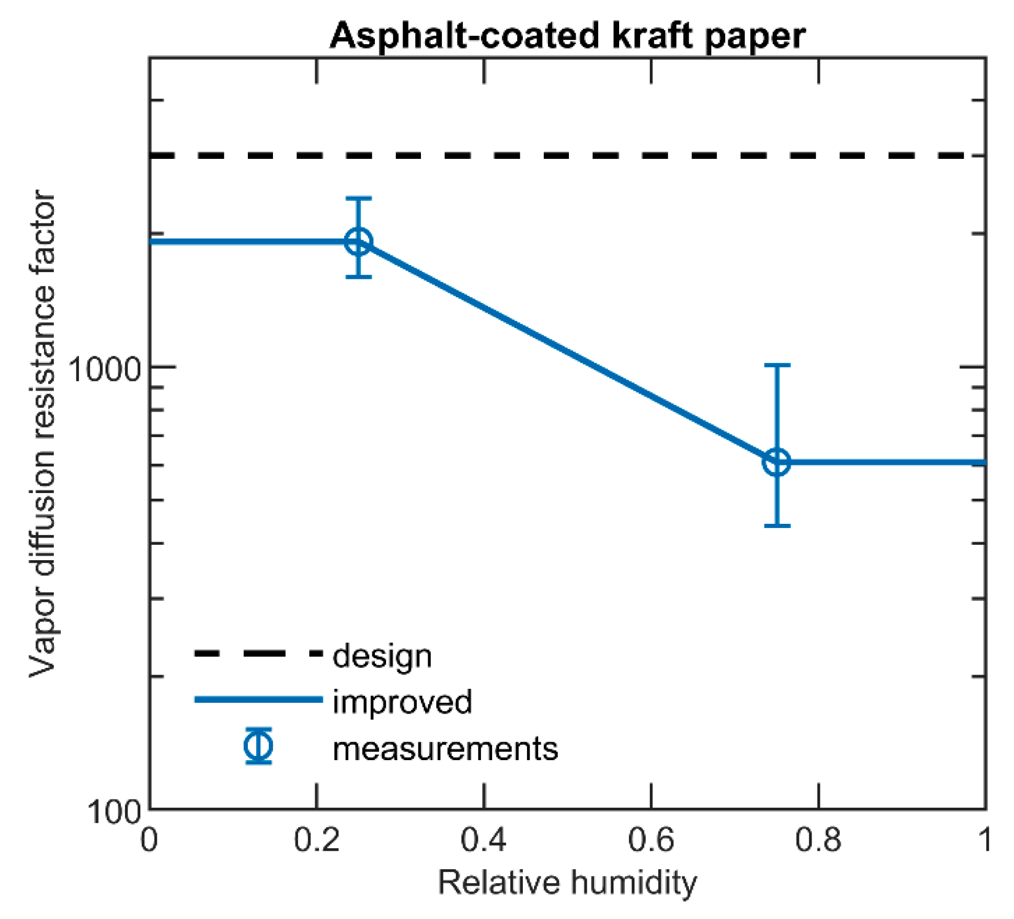
4.1.5. Asphalt-Coated Kraft Paper

Similar to the OSB, the laboratory measurements indicated that the kraft paper was more vapor open than literature values (see Table 2). The WUFI default kraft paper used in the design case had permeance of 66 ng Pa−1 s−1 m−2, already above that required for a Class II vapor retarder, but still not open enough. The only value changed from the design value for kraft paper was the water vapor permeance.
Laboratory values presented above were transformed into vapor diffusion resistance factors for a material 1 mm thick, as typically used in WUFI modeling, and are plotted in Figure 6 with the improved model and generic WUFI kraft paper values.

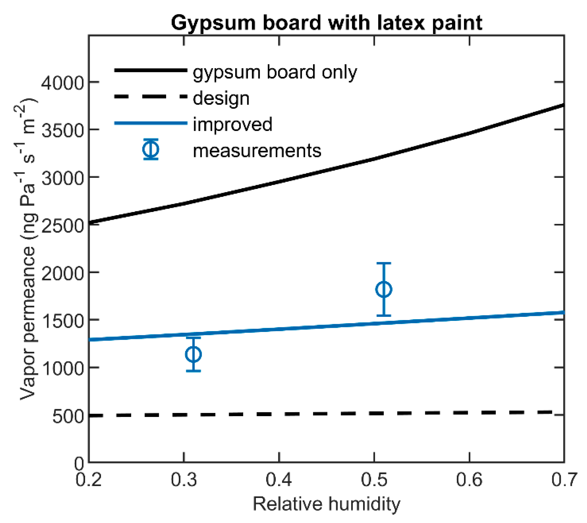
4.1.6. Latex Paint on Gypsum Board

Literature values for permeance of paint layers on gypsum vary widely. In our model exploration we found the reduction of the kraft vapor diffusion resistance factor to laboratory measured values was still not enough to give good agreement with measured data. This prompted another wet/dry cup permeance measurement of the combination gypsum and paint from our experimental test hut. Those results show that the paint had almost no effect on moisture movement. We reduced the sd-value for the interior surface from 0.32 m to 0.073 m for the improved model (based on the mean of the wet cup and dry cup values). Figure 7 plots the measured permeance values along with the permeance for unpainted gypsum from the WUFI database.

4.2. Changes in Simulation Results from Improvements

The net effect of these changes is to raise the overall OSB moisture level for each wall. The most significant increase occurred in walls with the kraft vapor retarder which were more exposed to the interior moisture during winter. The No CI walls were the most affected and approached the 20% MC limit during the winter. Figure 8 plots the OSB MC in all the north walls, like the plots in Figure 3b and Figure 4, but using the improved material properties.
In a different overview of these changes Figure 9 presents a bar graph of the maximum OSB MC over the two-year period for all 16 walls, comparing the design values with the improved model results just described.

5. Comparison of Improved Simulations with Measurements

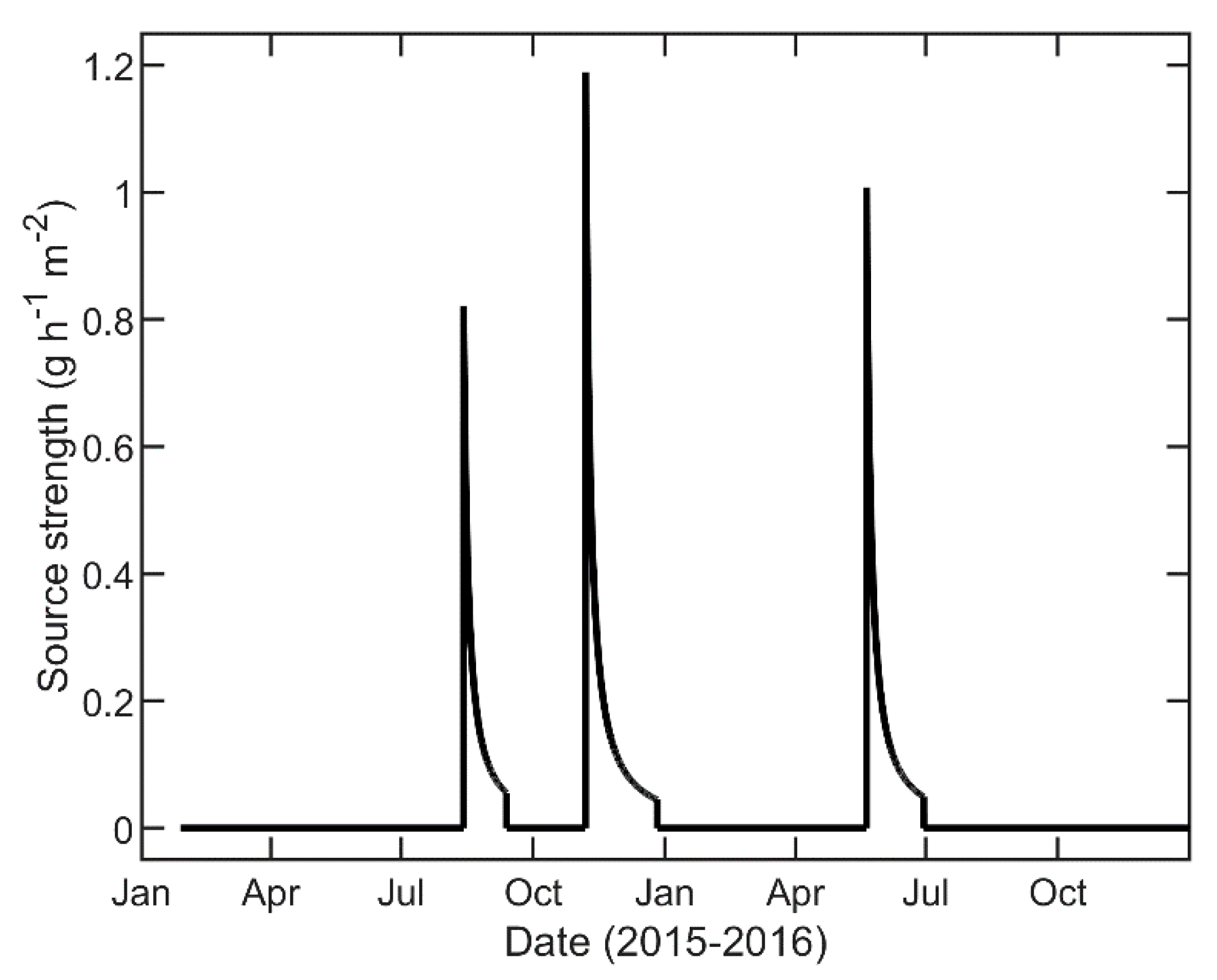
5.1. Model Adjustments to Facilitate Comparison

In order to facilitate comparison of model predictions with measured data, four additional changes were made to the model. First, the OSB was broken into three different layers, but the overall depth was maintained, thus the center layer had a depth of 6.1 mm, while inside and outside layers of 2.5 mm were added. This helps in two ways. First, it allows better resolution of the MC inside the OSB. Rather than getting the average value of one thick layer we can report the MC of each of the three layers. The inside or outside of the OSB may have a higher MC, exposing the OSB to the possibility of moisture damage, even while the overall MC remains low. Second, this helps the model comparison to measured data because the moisture pins used to record the MC of the OSB were screws which penetrated the OSB full depth. These pins measure the path of least resistance through the OSB, thus measuring the highest MC. In the model comparison we picked the highest MC of the 3 model OSB layers to compare with the measured value. In most of the plots to follow we continue to adjust the initial moisture content of each layer to match that at the end of the simulation. Finally, when all the adjustments are made and we are directly comparing the model to measured data, we set the initial MC of the OSB to the measured data.
Second, a minor model change facilitated the temperature comparison. The temperature sensor was attached to the inside surface of the OSB, providing a relative humidity and temperature reading in the cavity 5 mm from the OSB surface. Thus a 5 mm air layer was added (without additional moisture capacity) between the inner OSB surface and the fiberglass. A WUFI monitor was placed in the outer layer of the fiberglass, right next to the air layer, to record the temperature and humidity model predictions for comparison to this sensor.
Third, for comparison to measured data we used actual weather data, rather than the design values. Both indoor and outdoor conditions were monitored and used to create custom weather files for the two-year period. Winter indoor humidity values were maintained using a humidifier at 42% the first year and 34% the second year. Full details on the instrumentation and weather conditions is provided in [5]. Not mentioned in that report was the source of the solar data which came from the SOLRAD network station in Madison, which is maintained by NOAA’s Global Monitoring Laboratory. These changes in boundary conditions of course changed the model output. The effects of these first three model changes are illustrated in Figure 10 which again shows the OSB MC, this time the highest of the three layers, for all north walls. The primary difference from Figure 8 results from the new boundary conditions.
Most notable in this output is the effect of the kraft vapor retarder which increases the No CI case briefly above 27% MC level the first winter when the RH was 42% indoors, see Figure 10a. However, the kraft also allows the walls to dry inwards during the summers. This small effect can be seen when comparing the dashed line of XPS-poly with XPS-kraft after July 2016 in Figure 10b.
Finally, the fourth change accounts for the water injections which were done at three points during the two-year experimental study. These injections were intended to stress the walls and yield insight on how well different walls dried out. Modeling of these injections was explored in a previous study [36]. In summary, each test cavity received 40 g of water per day over a multiple day period: three days in fall, five days in winter, and four days in spring. These injections were modeled as a moisture source in the inner half of the inner OSB layer. The injection strengths are plotted in Figure 11.
These water injections produce a local variation in OSB moisture content that cannot be directly captured in the one-dimensional WUFI model. The average value of the two sensors outside the field of the paper towel was generally used as the reference measured data to compare with model prediction. Thus, we are modeling the OSB outside the area of the wetted towel with the moisture source representing the redistribution of water from the paper towel into the modeled area. The effect this injection had on the model prediction is illustrated in Figure 12, which shows wall 3, the MW kraft N case. This plot includes model predictions for the design case, the improved material properties case, adding the real weather, and finally adding in the water injections, all illustrated in the same north facing insulated wall. Inspection of Figure 12 reveals the same overall increase in OSB MC moving from design to the improved material properties that we have already noted. Further, again as we have seen, using the actual boundary conditions causes higher MC during winter, but lower MC during summer. The effects of the water injection were most noticeable during the winter injection which was the strongest. In this example case with MW insulation the wall quickly dries out and the OSB MC returns to that of the real weather example after a period of time which depends on the strength of the injection and the ability of the wall to dry out. Figure 13 provides two more example cases with wall 1 (No CI, kraft N) on left and wall 7 (XPS, poly N) on right. In Figure 12 and Figure 13 the initial MC of the OSB was directly set to the measured value at the start of the simulation for the ‘with injection’ case.

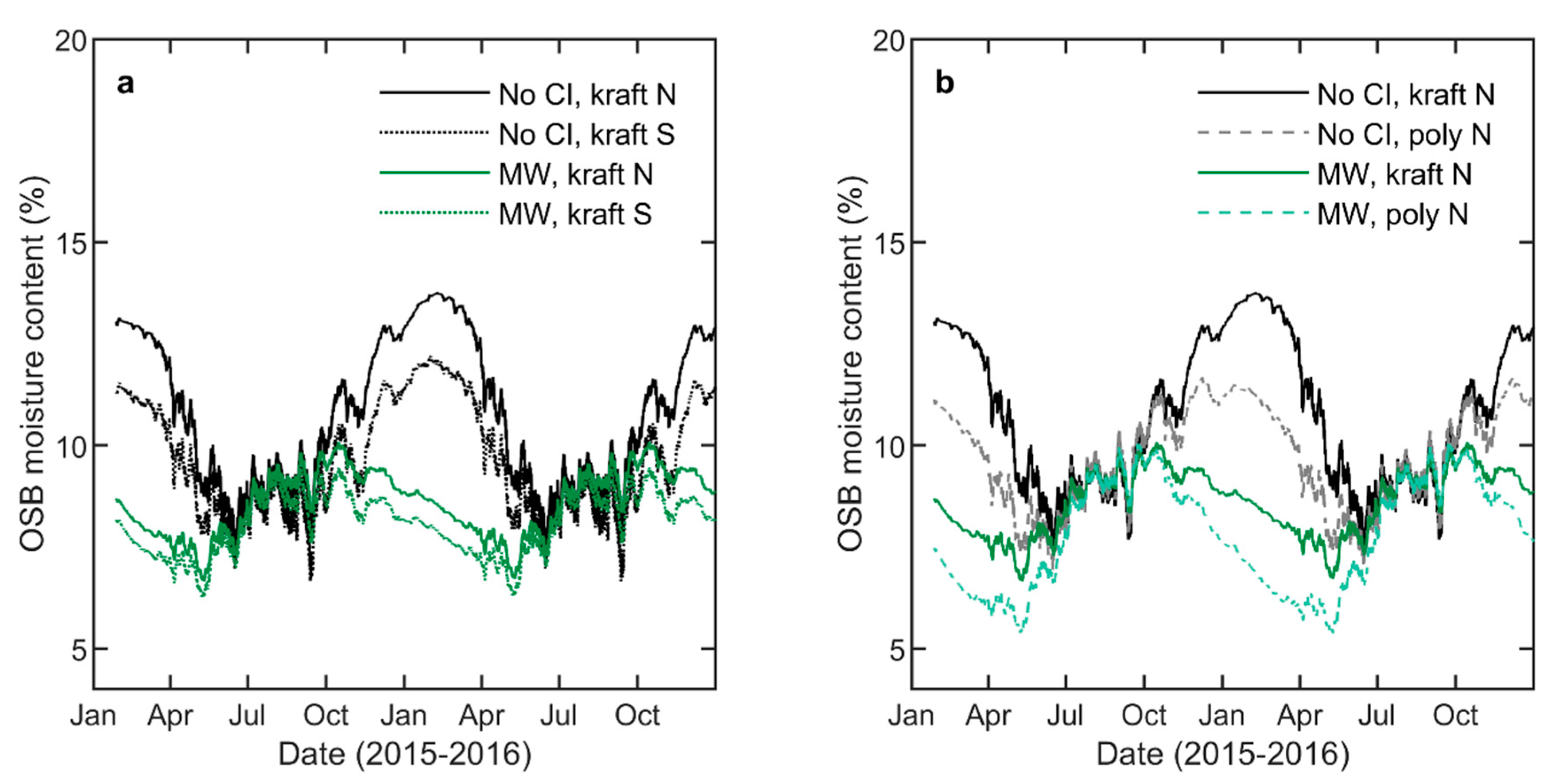
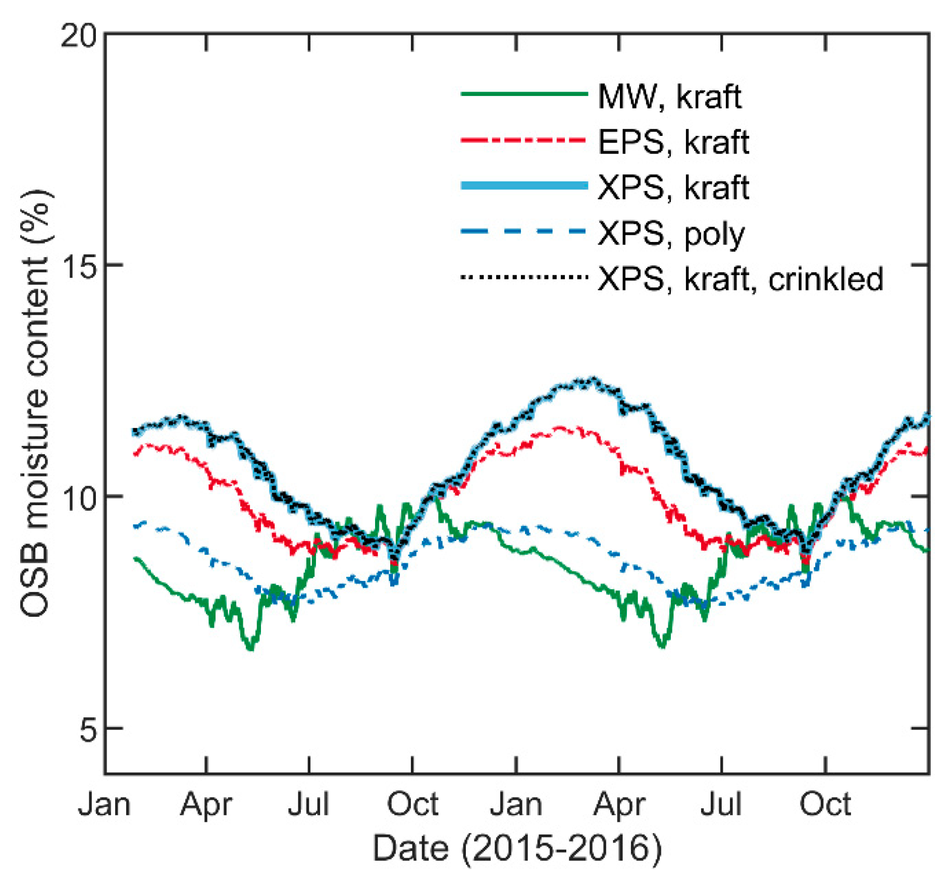
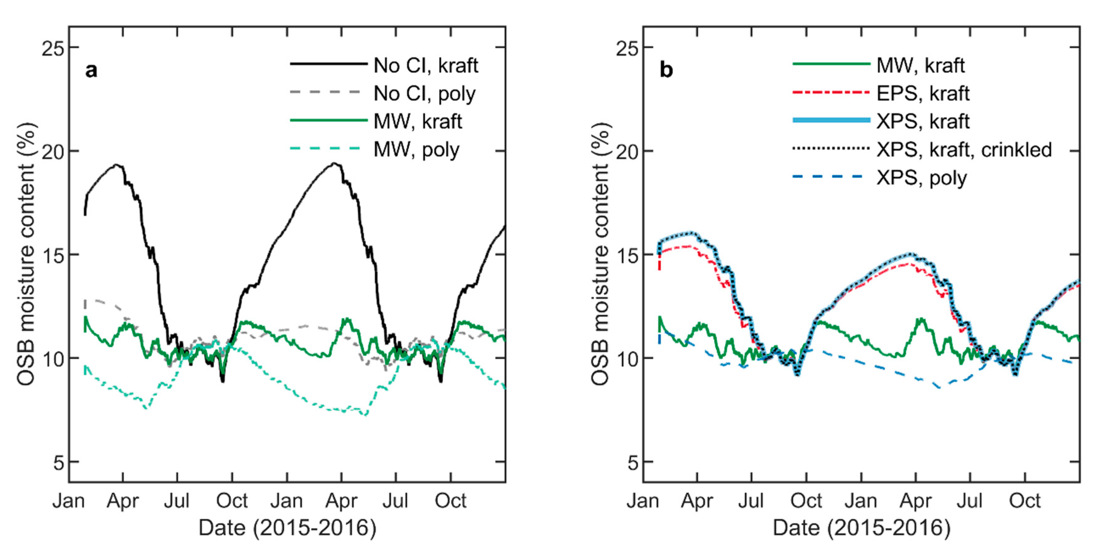
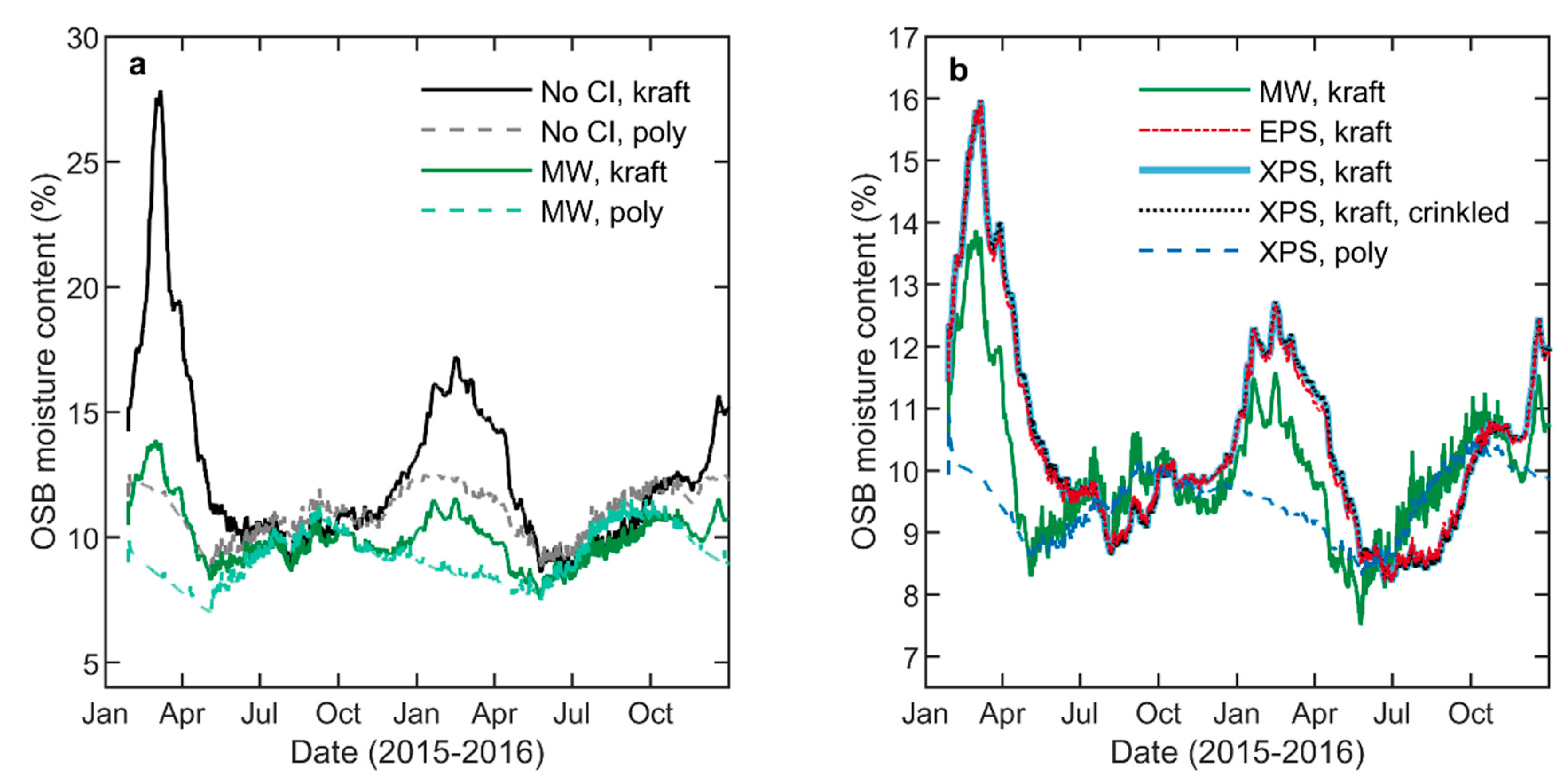
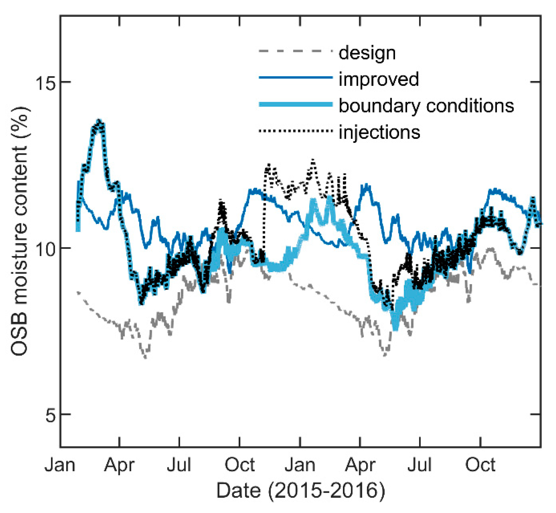
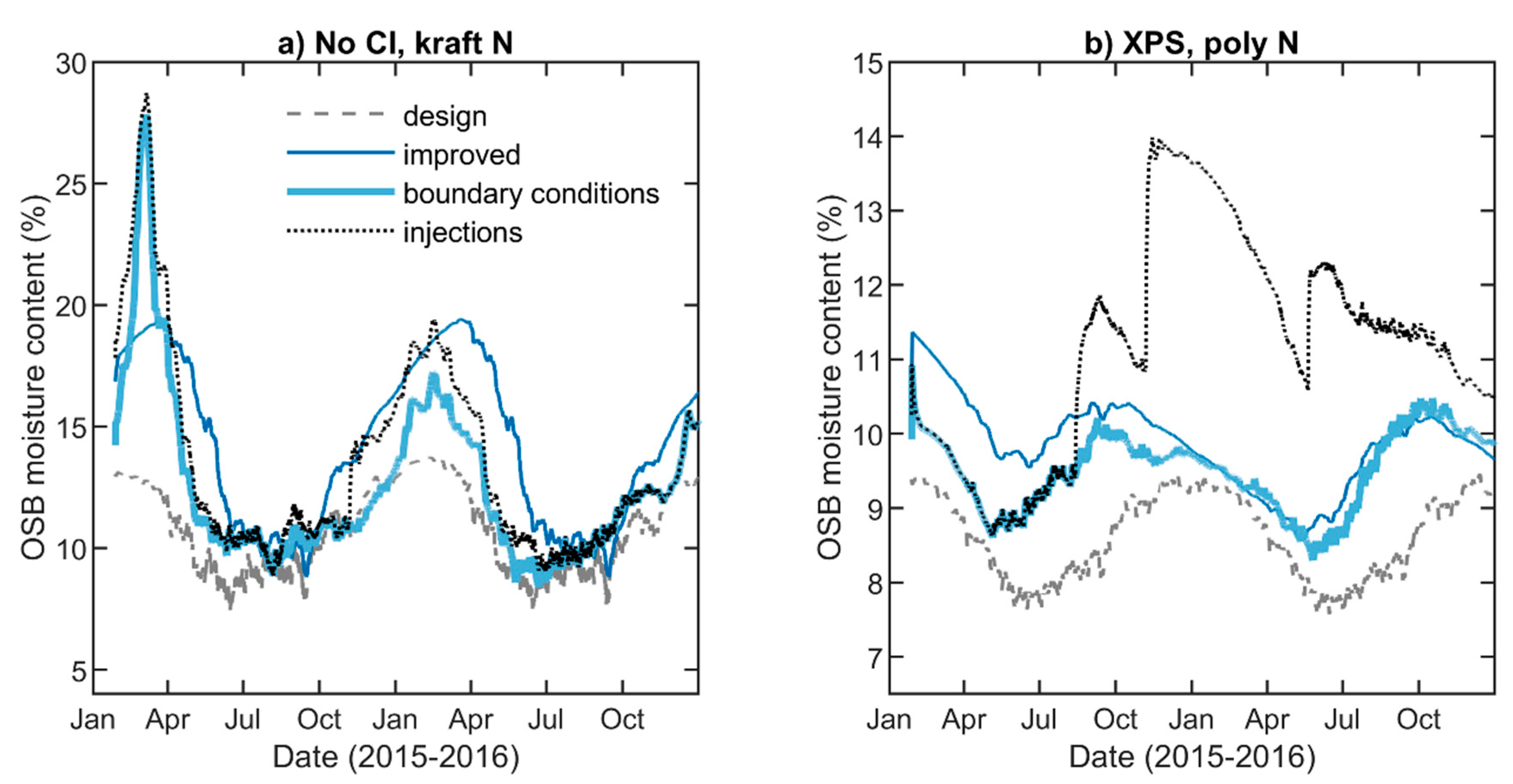
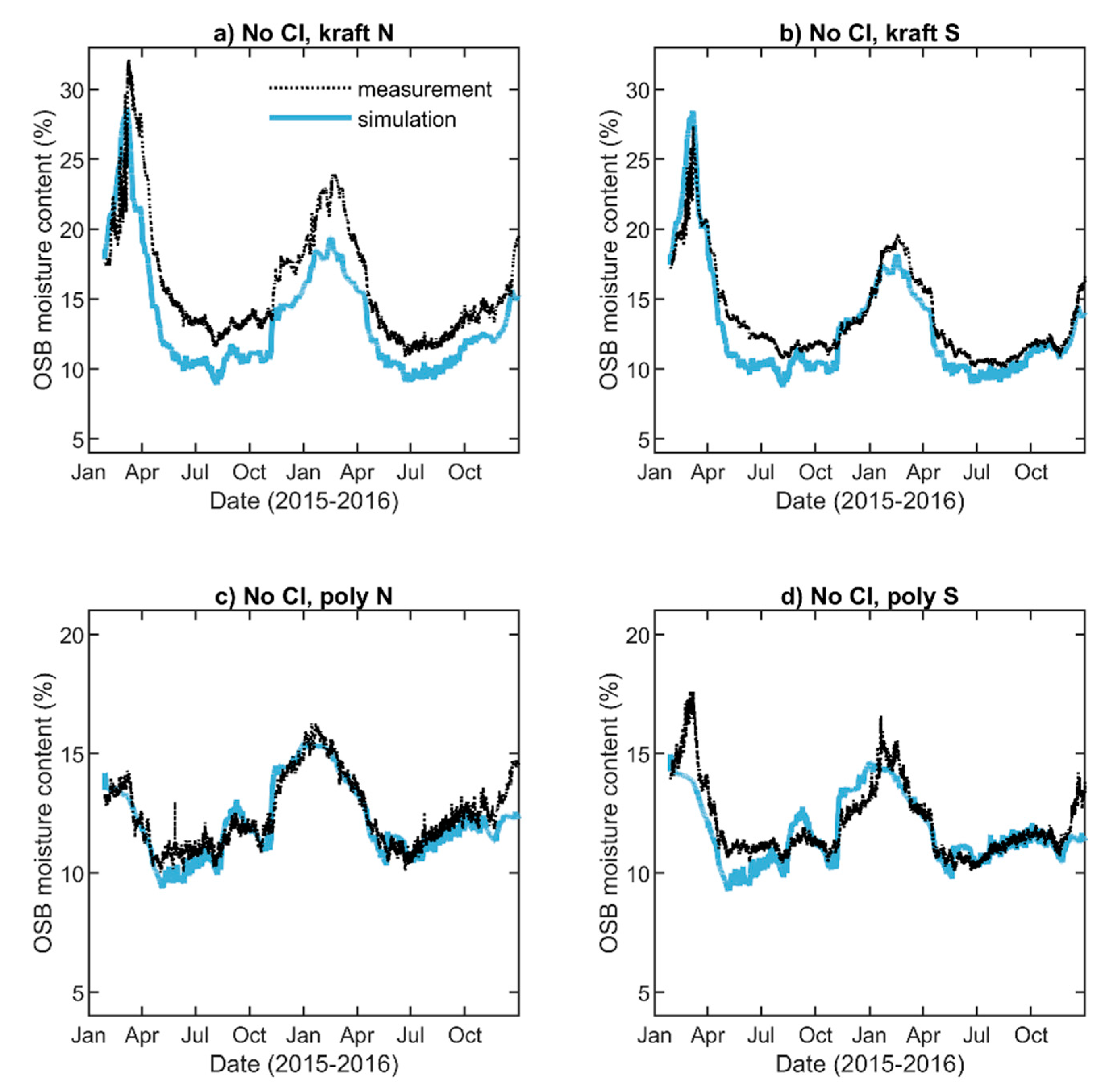
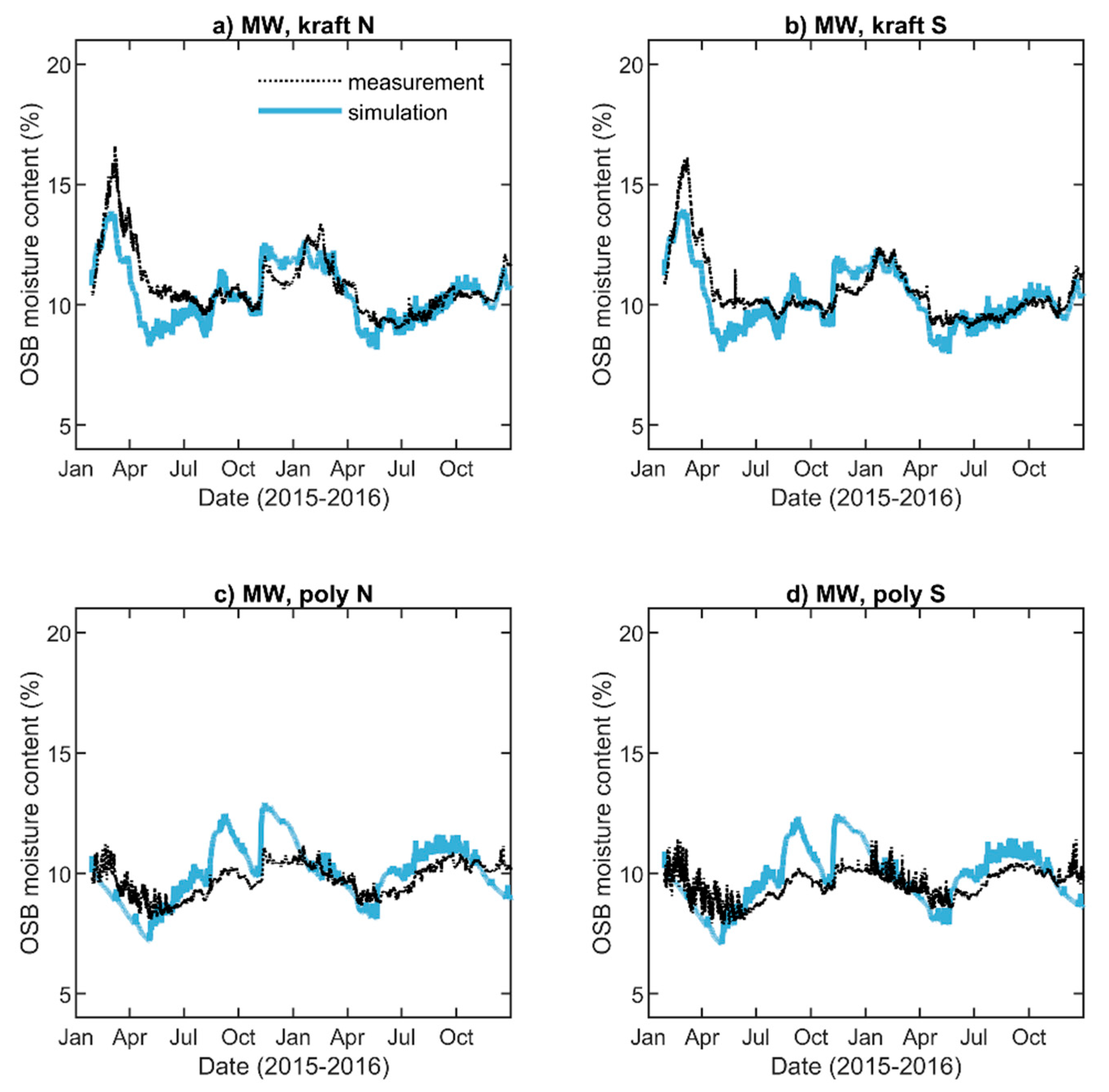
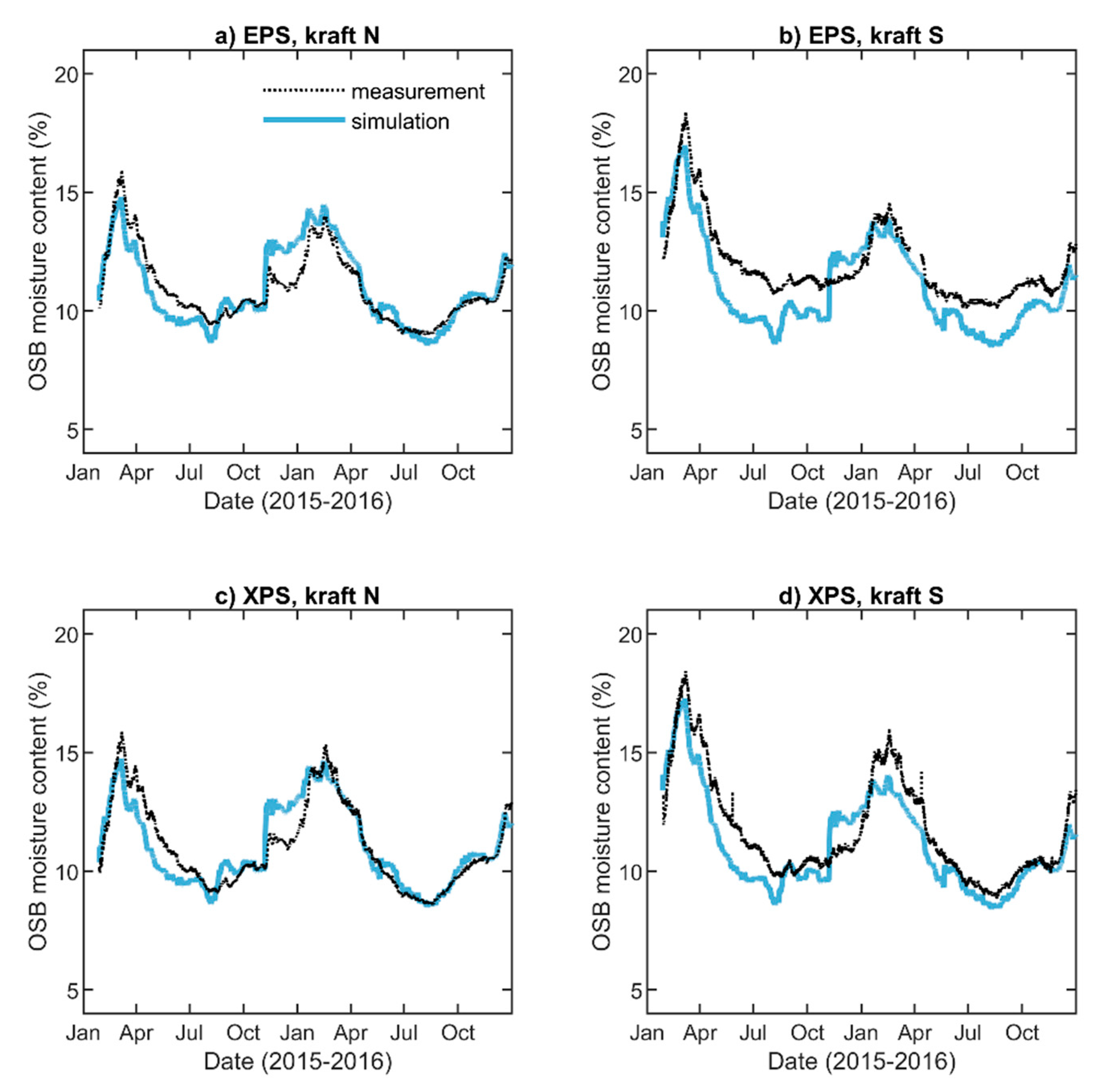
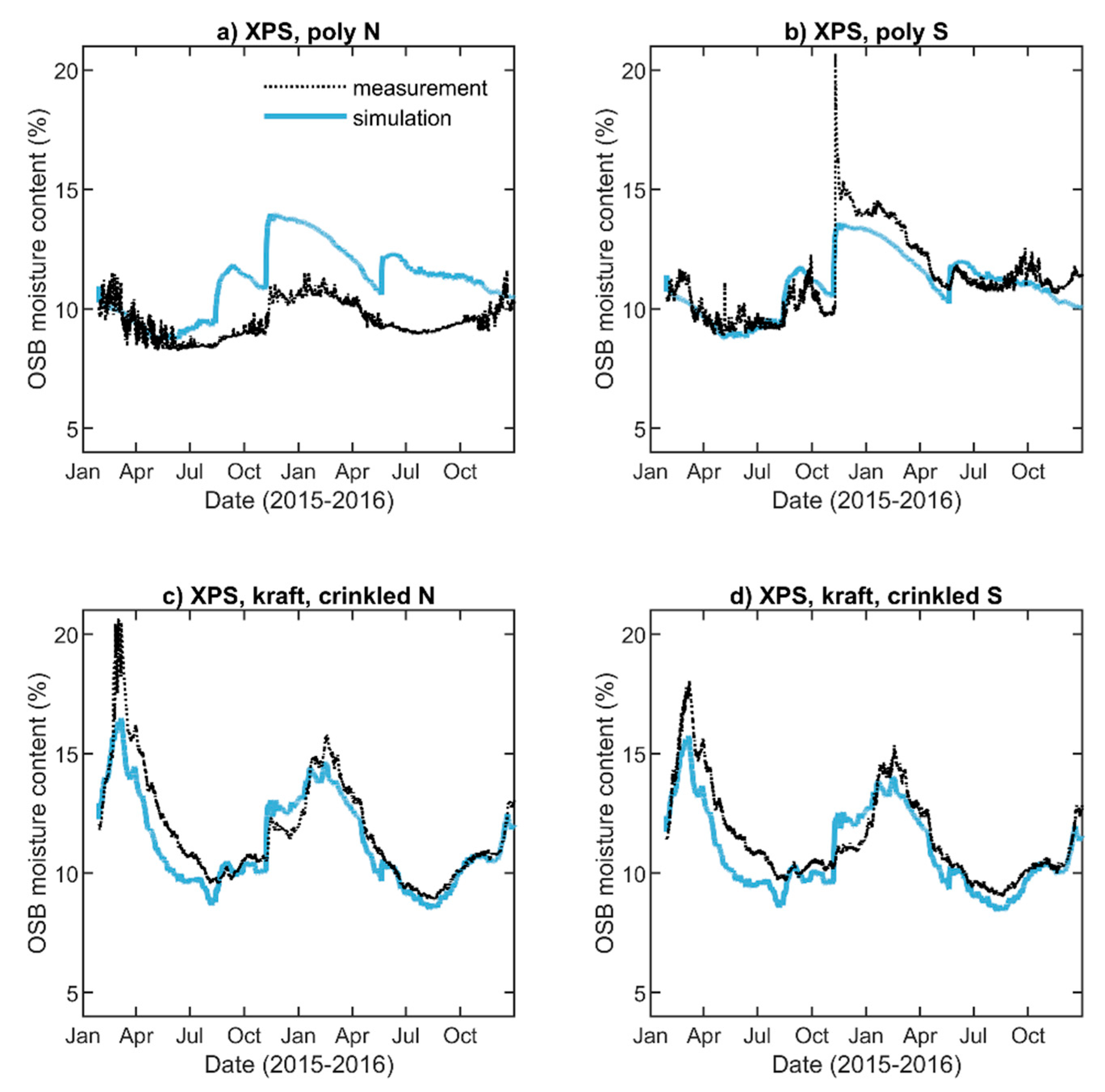
5.2. OSB Moisture Content

Given these model adjustments we now compare the best WUFI model predictions (which include the improved material properties and changes to facilitate data comparison) to the measured data for all 16 walls in Figure 14, Figure 15, Figure 16 and Figure 17. This first set of comparisons examines the OSB MC as we have done while exploring the design model. Each individual figure contains 4 plots, with the south and north versions of each wall right next to each other for easy comparison.
The fit between model and data will be examined numerically below (Table 3) through use of the root mean square error (RMSE) and a scaled error function. Additionally, we also plot select temperature and relative humidity values to visually compare model predictions for this measured data.

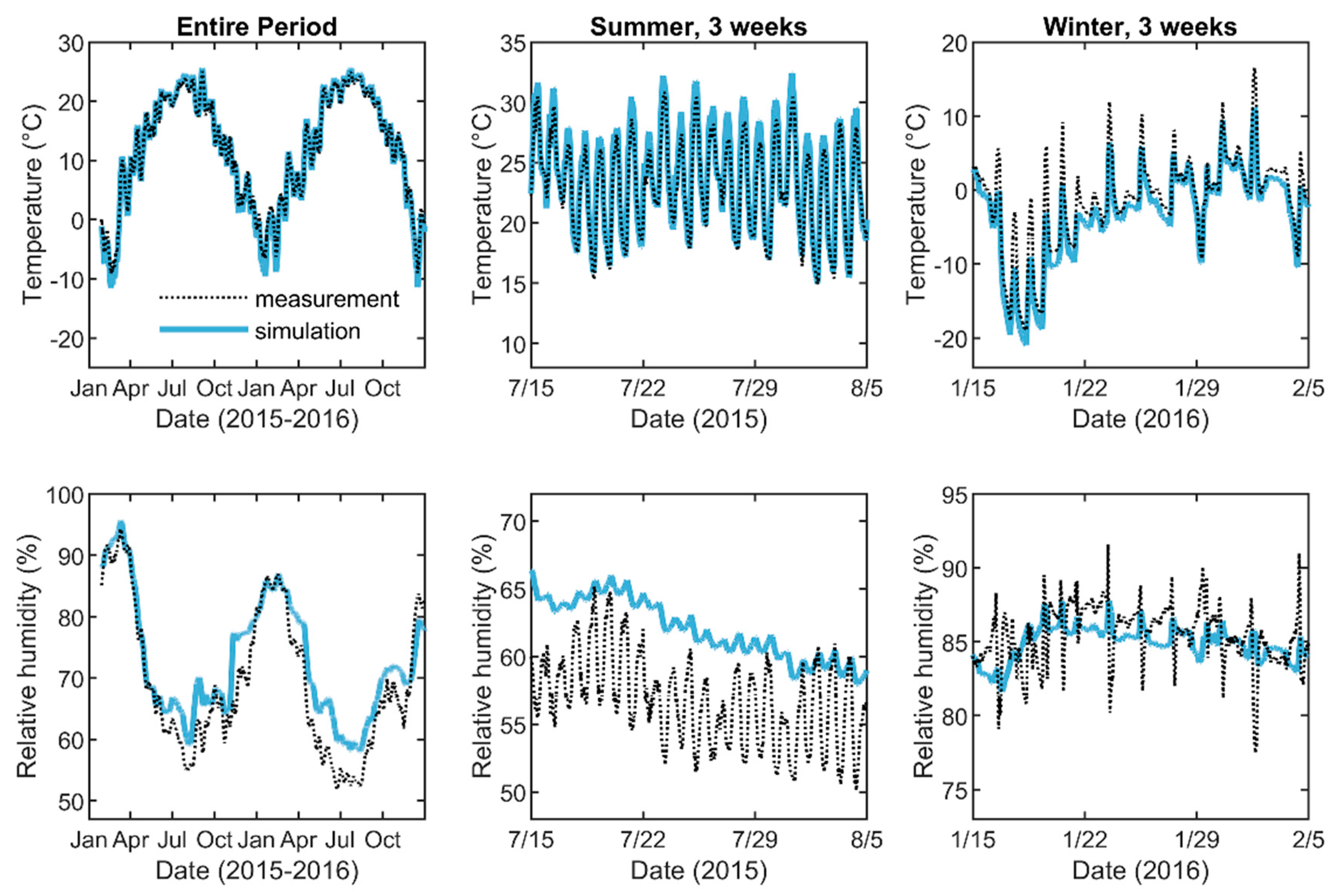
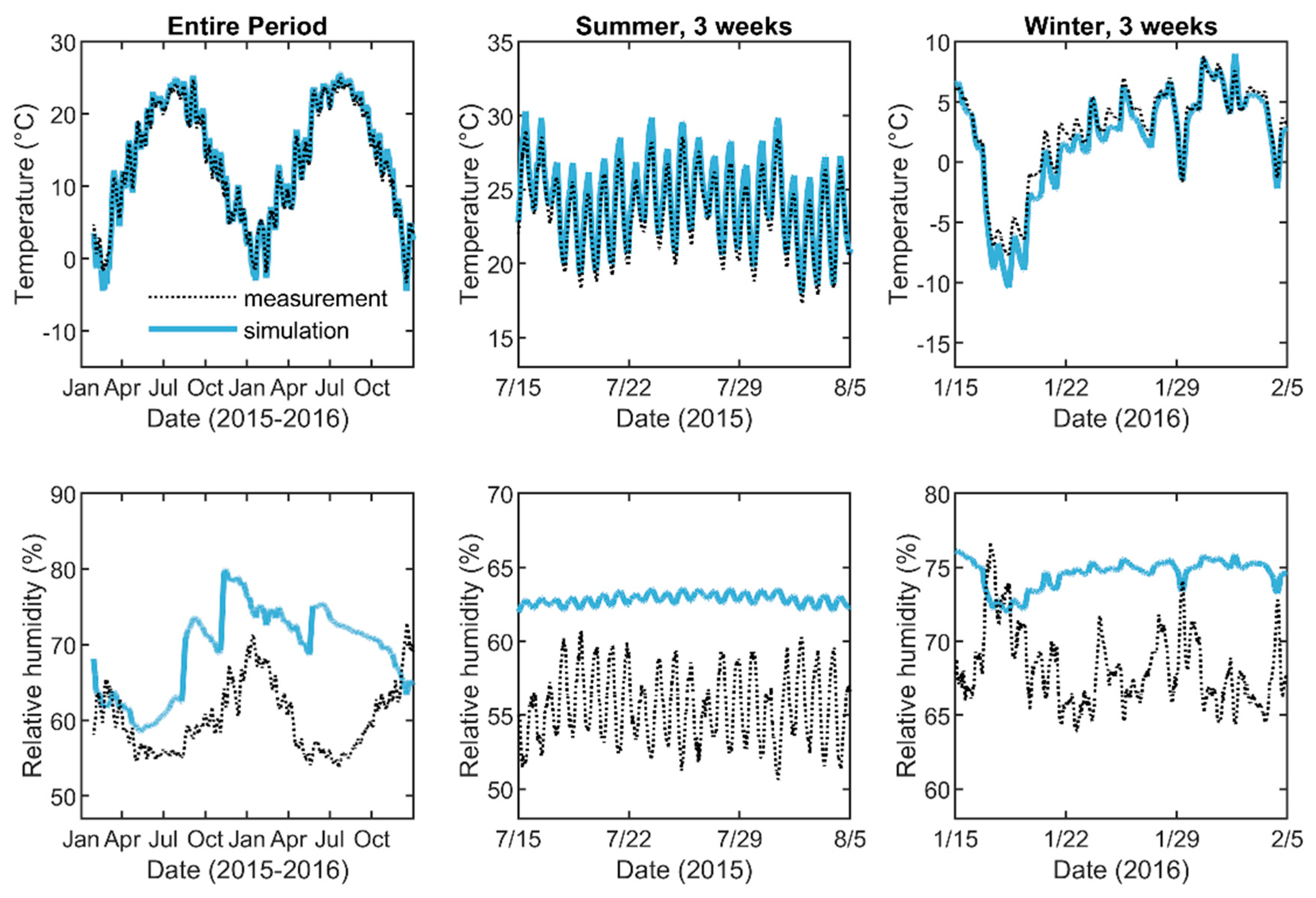
5.3. Temperature and Relative Humidity

An overview of the relative humidity and temperature for the No Cl, kraft S wall is plotted in Figure 18. On top is the temperature and bottom is relative humidity. The left column is full two years of data; the middle and right columns are close-up values during summer and winter. Figure 19 is a similar plot but for the XPS, poly N wall. The temperature prediction still tracks the data well, but the RH is too high, just as the XPS, poly walls showed OSB MC higher than the measured data in Figure 17. Quantitative summary data for all walls is provided in Table 4 below.

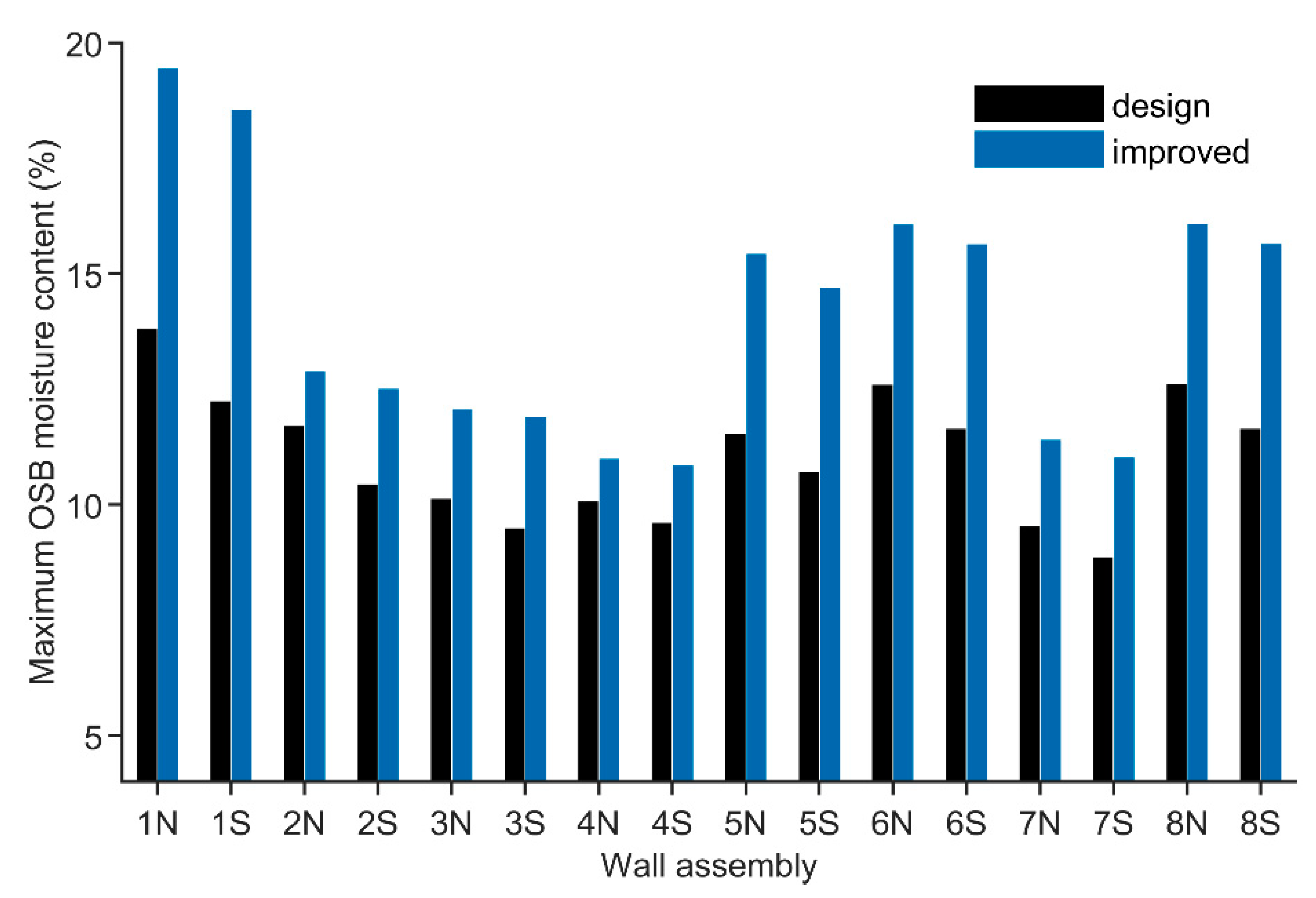
5.4. Quantitative Comparison of Simulations with Measurements

We use the root mean square error (RMSE) to quantify the difference between the model prediction and measured data. But there are three different measurements available: OSB MC (%), temperature (T, °C), and relative humidity (RH, %). We use a simple function to combine the three errors to indicate the overall goodness of fit. Since these errors have different magnitudes, they are scaled by the error associated with each measurement: T was measured to ±1.2 °C, RH to ±5%, and OSB MC to ±1.3%. The RMSE was calculated across all two years of data for each data type, then divided by the error for that type, and then added with more weight given to the OSB measurement as in Equation (1):
Scaled error = 50 × RMSEMC/1.3 + 25 × RMSET/1.2 + 25 × RMSERH/5
On this scale a value of 100 would indicate the simulation results are just within the errors from measurement. More weight was given to the OSB measurement because there were two sensors measuring OSB moisture content and moisture content is more important for assessment of durability. Table 3 provides the summary of the scaled error for all 16 walls for the WUFI model just explored in Figure 14, Figure 15, Figure 16 and Figure 17. This scaled error will be used to evaluate the effects of parameter changes in the sensitivity analysis that follows. Lower scaled error indicates a better model fit to experimental data.
Table 4 presents the RMSE of each component of the scaled error, along with the overall scaled error, for all south walls to provide insight into the typical error for each of the measured values.

6. Sensitivity Analysis
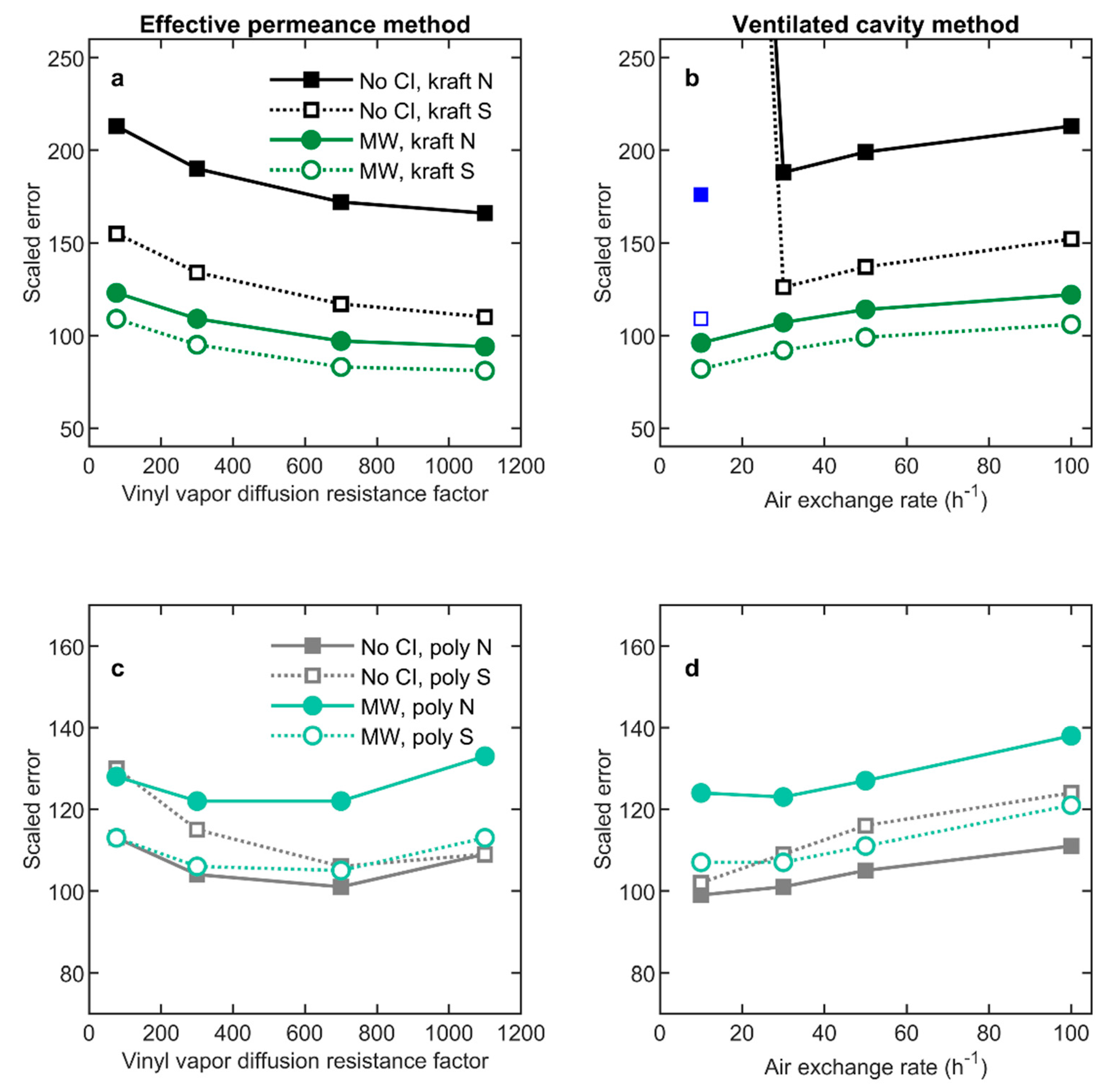
6.1. Vinyl Siding

Vinyl siding was modeled using an effective vapor permeance, so we explore this first. Then we explore the alternative method for modeling the vinyl siding by introducing an air layer behind the vinyl with various air changes per hour (ACH) with the exterior.

6.1.1. Effective Vapor Permeance

Walls 1 to 4 were most affected by the vapor permeance of the vinyl siding since they have either no exterior insulation or vapor open insulation. We thus report scaled error for these 4 walls using µ-values of 76 (design), 300, 700, and 1100 to survey values on either side of the improved model choice of 700. Figure 20a,c plots the result of the model runs with different effective permeance for the vinyl layer in two groups, with kraft paper vapor retarder walls on top and polyethylene vapor retarder walls on bottom.
The kraft walls which have ability to dry inward during late spring and summer show a modest improvement with increasing vapor diffusion resistance factor beyond 700, while the polyethylene walls do not. The WUFI predicted MC in kraft walls dries somewhat faster than measured data once the spring drying starts, and the higher vinyl resistance values slow down that drying, resulting in the lower RMSE.

6.1.2. Ventilated Air Cavity

To study the alternative method for handling air flow through the vinyl siding the model was changed to add a 5 mm air layer (without additional moisture capacity) between the vinyl and the WRB. A constant air exchange source was placed in this air layer to simulate that air flow. The vinyl itself had its µ value set to 2450. A series of WUFI runs were undertaken with different air changes per hour: 100, 50, 30, 10. The scaled error versus ACH values for walls 1–4 are plotted in Figure 20 right (b,d). Note that an additional run at 10 ACH for the No Cl, kraft walls was required with the numerical grid density increased to 500 and the air layer changed to the 5 mm air layer which includes additional moisture capacity. Those extra results are shown as separate points (blue square open and closed) without a line connecting them to the other results.
Figure 20b,d illustrates the general improvement of model prediction with the reduction in ACH until the simulation stops working well. Inspection reveals a pattern like the effective permeance sensitivity study. The kraft walls again show a modest improvement with decreasing ACH below 30, while the polyethylene MW walls do not.
The air layer method of handing the air flow through vinyl siding is not necessarily robust at low ACH values, but it can work. We had already increased the water storage capacity of the vinyl for the improved model. Without that change the ACH method of handing vinyl air flow fails at 30 ACH, just as it did at 10 ACH. These failures are marked by the dramatic rise in scaled error (to near 1000) and associated convergence failures (over 300). This simulation failure is a result of too much water in the small air space. WUFI provides a solution using the standard air layer which has a much higher water capacity (higher than air really can hold). The combination of significant water storage in the vinyl layer with the extra water storage in the air layer allows the simulation to work without convergence failures.

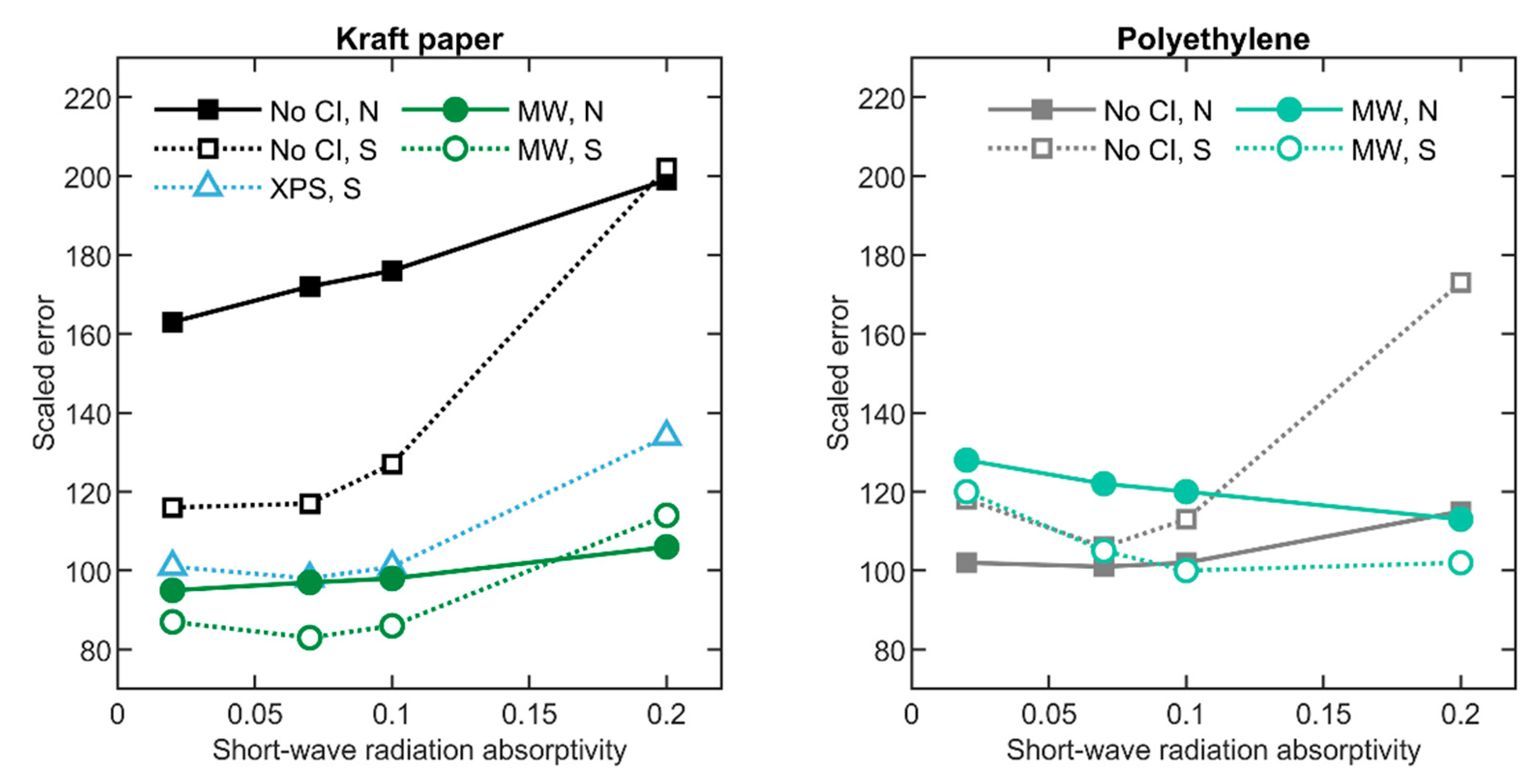
6.2. Short-Wave Radiation Absorptivity

As previously mentioned, the model is sensitive to the exterior wall short-wave radiation absorptivity, and we did not have a measured value for this parameter. The sensitivity study ranges from the design value of 0.2, down to 0.1, 0.07, and 0.02 to cover a wide range of absorptivity values. Recall that 0.07 was the value chosen for the improved model. Figure 21 plots the scaled error versus these absorptivity values for select wall assemblies. In general reduction of the short-wave absorptivity was warranted but below 0.1 different walls show different behavior.

6.3. Exterior Surface Heat Transfer Coefficient
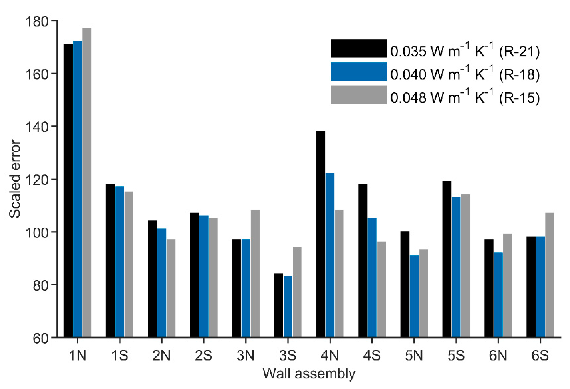
The improved model used a constant boundary layer air resistance for the exterior wall, but WUFI allows this resistance to vary with wind speed. This section examines the effect of turning this setting on. We did not modify the default WUFI equation which computes the resistance based on wind speed. Table 5 presents scaled error for select walls with the wind setting on. It is like Table 3, in that it has the scaled error for the improved model (base) wall, but adds a column labeled ‘wind’ and one labeled ‘diff’ which gives the percentage change from the base case. Overall, there is a slight improvement in the model when the wind can vary the external thermal resistance.

6.4. Fiberglass

The simulation is also sensitive to the thermal resistance of the fiberglass. The sensitivity study includes three thermal conductivity values, reflecting a range of possible values that could depend on the quality of fiberglass batt installation: the highest resistance was the same as that in the design case, with conductivity of 0.035 W/m K (R-21), the improved model case of 0.040 W/m K (R-18), and a low resistance case of 0.048 W/m K (R-15). Figure 22 plots a bar graph of the scaled error in these three cases for select walls. Inspection of Figure 22 reveals no clear pattern in scaled error but modeling modestly lower levels of effectiveness for the fiberglass insulation, as in the improved model, produces good results based on overall average error.

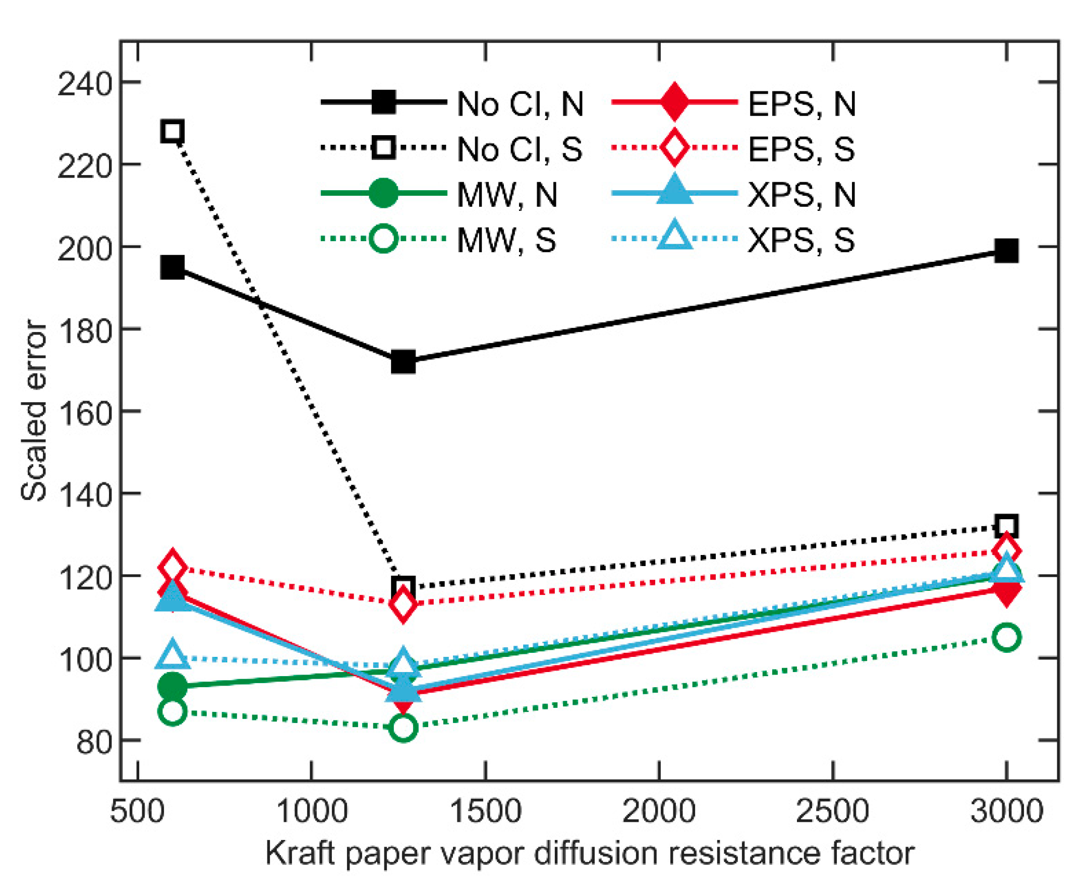
6.5. Asphalt-Coated Kraft Paper

The kraft paper vapor diffusion resistance factor was decreased based on laboratory measurements. The sensitivity values explored are the design µ value of 3000, improved model values which ramped from 1919 (at 25% RH) to 609 (at 75% RH), and a constant 600 value. These results are presented for walls with kraft vapor retarder in Figure 23. The improved model value is plotted at the average µ value of 1264. Inspection of Figure 23 reveals there rarely is an improvement in the scaled error when reducing the resistance below the improved model value to 600.

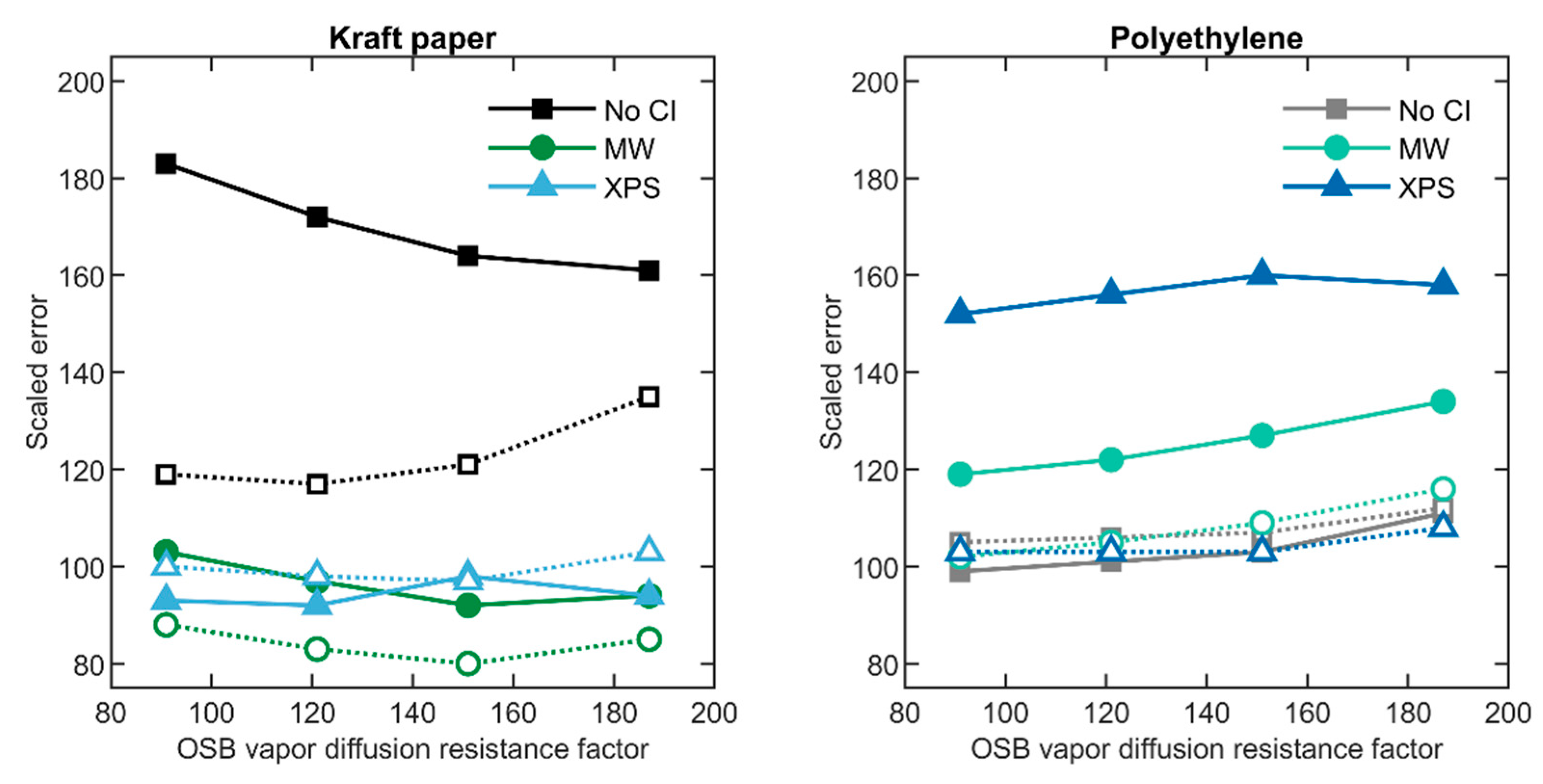
6.6. Oriented Strand Board

The improved model used an OSB vapor diffusion resistance factor curve below that of the low density WUFI database OSB. We tested these two values, improved and design, plotted at their 50% RH values as 121 and 187 in Figure 24. The results show the reduction to the laboratory measured values works well, but the results were not particularly sensitive. To explore this further Figure 24 includes two additional points, one 75% of the improved model, and the other 125% of that model, plotted at µ values of 91 and 151.

6.7. Extruded Polystyrene

Earlier we noted that the design case XPS, poly wall models did not dry out as fast as the measured data. We suspect that there is additional drying with air movement between the XPS and OSB. This air movement would in theory be enhanced by the crinkled WRB. With the existing data set there is no good way to distinguish the effects of the crinkled from the plain WRB, but we used an effective permeance for the XPS in the improved simulation to represent the drying benefits which could be due to this air movement. Further empirical investigation of air movement between exterior insulation and sheathing is warranted but outside the scope of this study.
The sensitive study starts with the WUFI North American database vapor diffusion resistance factor value of 171 and includes values of 75% (59) and 125% (99) of the improved model value of 79. Note that literature values vary from 94 to 208 [22,23,38,39]. Scaled error for these four model values are plotted in Figure 25 for walls with XPS exterior insulation. Clearly the walls with polyethylene vapor retarder benefit from the lower XPS resistance factor, and 79 would be a reasonable value. The walls with kraft vapor retarder show little sensitivity to the XPS values as expected since they can dry to the inside.

6.8. Discussion

Two of the sensitivity study results deserve further discussion. First, the effective permeance of the vinyl siding was much lower than expected. This is likely because many of the previous studies on vinyl siding examined installations over furring strips, which created an air gap between the siding and the insulation or WRB. This air gap significantly increases the air flow behind the vinyl siding. In contrast, our vinyl siding was installed directly on the WRB or exterior insulation. Although some studies [40] have found directly applied vinyl siding to be quite air permeable, Tsongas reports forensic investigation of damage in multifamily housing walls with directly applied vinyl siding [41]. He concludes that when damage occurs in these installations a significant cause is the impermeable vinyl siding, which appears to be relatively airtight and impedes drying to the outside. Our findings reinforce the conclusion that directly applied vinyl siding can be significantly less air permeable than previously thought. Second, the permeance of the XPS was higher than expected. The evidence was that XPS covered walls challenged by water injection dried out faster than the design case WUFI model. The concept of effective permeance is not typically applied to XPS, but further research into moisture flow under field installation conditions is warranted. Using the ASTM standard water vapor transmission tests, which feature sealed edges, may not capture all the relevant physical processes occurring in full-scale field installations of exterior insulation. Further evidence for an increased XPS effective permeance is found in the work of Boardman et al. [42].

7. Conclusions

Agreement between one-dimensional WUFI hygrothermal simulations and field measurements was improved by changes in material properties and by using measured indoor and outdoor boundary conditions. The three most important material properties in the improved model were the effective permeance of the vinyl siding, the permeance of the kraft paper interior vapor retarder, and the effective permeance of the exterior XPS insulation. The 40-perm design value for effective permeance of vinyl siding was too high for our case. Predictions improved with 10 times more vapor diffusion resistance. In addition, during cold weather and high indoor RH, the kraft-facing of fiberglass cavity insulation, being more vapor open than expected, resulted in significant moisture accumulation in the OSB. This accumulation was reduced by adding exterior insulation. The measured vapor permeance of the kraft paper was considerably higher than the default value for kraft paper in the WUFI database. Finally, modeling of walls with XPS exterior insulation showed higher OBS MC than measured. A possible explanation is that slight airflow between the XPS and OSB increases the ability of the wall to dry out. Use of an XPS effective permeance improved the simulations. Given these changes, the difference between measured and simulated values of OSB moisture content, temperature, and relative humidity for the typical wall was on the order of experimental error in measured values.

Author Contributions

Conceptualization, C.R.B. and S.V.G.; methodology, C.R.B. and S.V.G.; software, C.R.B.; validation, C.R.B.; formal analysis, C.R.B.; investigation, C.R.B. and S.V.G.; resources, C.R.B.; data curation, C.R.B.; writing—original draft preparation, C.R.B.; writing—review and editing, C.R.B. and S.V.G.; visualization, C.R.B. and S.V.G.; supervision, S.V.G.; project administration, S.V.G. All authors have read and agreed to the published version of the manuscript.

Funding

This work was funded by the USDA Forest Service, Forest Products Laboratory, and APA—The Engineered Wood Association through Joint Venture Agreement 14-JV-11111136-054.

Acknowledgments

The manuscript was improved by helpful comments from Marshall Begel and Keith Bourne.

Conflicts of Interest

The authors declare no conflict of interest.

Appendix A. Property Data Used in Hygrothermal Simulations

The material properties used in the improved model are documented in sections specific to each material. When relevant the WUFI database entry used for design is shown as an entry in the additional ‘Design’ column. For OSB both the full improved model and WUFI design values are provided in additional separate tables for clarity. For those materials (Mineral Wool and Fiberglass) for which the thermal conductivity changes with moisture content the relevant table is included, otherwise the thermal conductivity is only adjusted using the thermal conductivity temperature coefficient.

Appendix A.1. Vinyl Siding—Installed Directly on Sheathing or Insulation—Effective Permeance

Table A1. Vinyl Siding property data—using effective permeance.
PropertyValueDesign
Thickness, mm1.11
Bulk density, kg/m3829
Porosity, m3/m310.001
Specific heat capacity (dry), J/(kg·K)2299
Thermal conductivity, W/(m·K)0.17
Thermal conductivity temperature coefficient, W/(m·K2)0.0002
Water vapor diffusion resistance factor70076
Table A2. Default water storage function (applies to vinyl with porosity = 1).
RHWater Content, kg/m3RHWater Content, kg/m3
000.935.72
0.50.4850.946.6
0.60.7240.957.77
0.71.120.969.41
0.81.880.9711.9
0.852.620.9815.9
0.94.030.9923.9
0.914.480.99531.8
0.925.03147.1

Appendix A.2. Extruded Polystyrene (XPS) Insulation

Table A3. XPS property data.
PropertyValueDesign
Thickness, mm25.4
Bulk density, kg/m328.6
Porosity, m3/m30.99
Specific heat capacity (dry), J/(kg·K)1470
Thermal conductivity, W/(m·K)0.025
Thermal conductivity temperature coefficient, W/(m·K2)0.0002
Water vapor diffusion resistance factor79170.56
Table A4. Moisture storage function.
RHWater Content, kg/m3
00
0.10.009
0.50.08
0.80.31
0.90.66
0.971.95
0.993.94
0.9997.09
17.77

Appendix A.3. Expanded Polystyrene (EPS) Insulation

Table A5. EPS property data.
PropertyValue
Thickness, mm38.1
Bulk density, kg/m314.8
Porosity, m3/m30.99
Specific heat capacity (dry), J/(kg·K)1470
Thermal conductivity, W/(m·K)0.036
Thermal conductivity temperature coefficient, W/(m·K2)0.0002
Water vapor diffusion resistance factor73.01
Table A6. Moisture storage function.
RHWater Content, kg/m3
00
0.10.004
0.50.031
0.80.12
0.90.26
0.970.77
0.991.55
0.9992.78
13.05
Table A7. Water vapor diffusion resistance factor.
RHµ-Value
073.01
0.173
0.267.34
0.361.93
0.457.17
0.552.55
0.648.39
0.744.65
0.841.04
0.937.83
134.8

Appendix A.4. Mineral Wool (MW) Insulation

Table A8. MW property data.
PropertyValue
Thickness, mm38.1
Bulk density, kg/m3128
Porosity, m3/m30.954
Specific heat capacity (dry), J/(kg·K)850
Thermal conductivity, W/(m·K)0.0322
Thermal conductivity temperature coefficient, W/(m·K2)0.0002
Water vapor diffusion resistance factor1.3
Table A9. Moisture storage function.
RHWater Content, kg/m3RHWater Content, kg/m3
000.9933.43
0.650.40.99587.9
0.80.70.999269.26
0.932.20.9995298.73
0.975.90.9999312.96
0.98121314
Table A10. MW thermal conductivity adjustment with water content.
Water Content, kg/m3Thermal Conductivity, W/(m·K)
00.0322
100.033
200.034
500.038
1000.043
2000.062
3000.09
4000.13
5000.18
6000.24
7000.32
8000.42
9000.54
9540.6

Appendix A.5. Spun Bonded Polyolefin Membrane (SBP)

Table A11. SBP property data.
PropertyValue
Thickness, mm1
Bulk density, kg/m365
Porosity, m3/m30.001
Specific heat capacity (dry), J/(kg·K)1500
Thermal conductivity, W/(m·K)2.3
Thermal conductivity temperature coefficient, W/(m·K2)0.0002
Water vapor diffusion resistance factor49.3

Appendix A.6. Spun Bonded Polyolefin Membrane with Crinkled Surface (SBPC)

Table A12. SBPC property data.
PropertyValue
Thickness, mm1
Bulk density, kg/m367
Porosity, m3/m30.001
Specific heat capacity (dry), J/(kg·K)1500
Thermal conductivity, W/(m·K)2.3
Thermal conductivity temperature coefficient, W/(m·K2)0.0002
Water vapor diffusion resistance factor65.6

Appendix A.7. Oriented Strand Board (OSB)

Appendix A.7.1. Improved Model

Table A13. OSB property data—improved model and Design values.
PropertyValueDesign
Thickness, mm11.1
Bulk density, kg/m3534575
Porosity, m3/m30.640.8625
Specific heat capacity (dry), J/(kg·K)12801880
Thermal conductivity, W/(m·K)0.08060.084
Thermal conductivity temperature coefficient, W/(m·K2)0.0002
Water vapor diffusion resistance factor1951182
Table A14. Moisture storage function—improved model.
RHWater Content, kg/m3RHWater Content, kg/m3
000.757.1
0.112.70.871.9
0.220.10.995.1
0.326.10.95112.7
0.4320.98126.6
0.538.61333
0.646.6--
Table A15. Water vapor diffusion resistance factor—improved model.
RHµ-Value
0195
0.25195
0.7547
0.840.8
140.8
Table A16. Liquid transport coefficient—improved model.
Water Content, kg/m3D (Suction), m2/sD (Redistribution), m2/s
000
71.97.37 × 10−137.37 × 10⁻¹³
3331.66 × 10−101.66 × 10⁻¹¹

Appendix A.7.2. WUFI Database Low Density (575 kg/m3) OSB Entries

Table A17. Moisture storage function—Design.
RHWater Content, kg/m3
00
0.4929.6
0.69555.2
0.90587.4
1333.5
Table A18. Water vapor diffusion resistance factor—Design.
RHµ-Value
01182
0.11182
0.21182
0.3525.5
0.4295.5
0.5187.5
0.6130
0.795
0.872.3
0.956.9
145.6
Table A19. Liquid transport coefficient—Design.
Water Content, kg/m3D (Suction), m2/sD (Redistribution), m2/s
000
71.37.24 × 10−137.24 × 10⁻¹³
333.51.65 × 10−101.65 × 10⁻¹¹

Appendix A.8. Fiberglass Batt Cavity Insulation (Used with Additional 5 mm Air Gap)

Table A20. Fiberglass insulation property data.
PropertyValueDesign
Thickness, mm135140
Bulk density, kg/m330
Porosity, m3/m30.0080.99
Specific heat capacity (dry), J/(kg·K)840
Thermal conductivity, W/(m·K)0.03980.035
Thermal conductivity temperature coefficient, W/(m·K2)0.0002
Water vapor diffusion resistance factor1.3
Table A21. Fiberglass thermal conductivity adjustment with water content.
Water Content, kg/m3Thermal Conductivity, W/(m·K)Design
00.03980.035
500.050.043
1000.050.049

Appendix A.9. Kraft Paper Facing

Table A22. Kraft paper property data.
PropertyValueDesign
Thickness, mm1
Bulk density, kg/m3120
Porosity, m3/m30.6
Specific heat capacity (dry), J/(kg·K)1500
Thermal conductivity, W/(m·K)0.42
Thermal conductivity temperature coefficient, W/(m·K2)0.0002
Water vapor diffusion resistance factor19193000
Table A23. Moisture storage function.
RHWater Content, kg/m3
00
0.50.6
0.81.8
0.92.6
0.973.5
111.2
Table A24. Water vapor diffusion resistance factor—improved model.
RHµ-Value
01919
0.251919
0.75609
1609

Appendix A.10. Polyethylene Membrane (PE)

Table A25. PE property data.
PropertyValue
Thickness, mm1
Bulk density, kg/m3130
Porosity, m3/m30.001
Specific heat capacity (dry), J/(kg·K)2300
Thermal conductivity, W/(m·K)2.3
Thermal conductivity temperature coefficient, W/(m·K2)0.0002
Water vapor diffusion resistance factor50,000

Appendix A.11. Interior Gypsum Board

Table A26. Gypsum property data.
PropertyValue
Thickness, mm12.5
Bulk density, kg/m3625
Porosity, m3/m30.706
Specific heat capacity (dry), J/(kg·K)870
Thermal conductivity, W/(m·K)0.16
Thermal conductivity temperature coefficient, W/(m·K2)0.0002
Water vapor diffusion resistance factor7.03
Table A27. Moisture storage function.
RHWater Content, kg/m3
00
0.5054.34275
0.716.15625
0.89611.3125
0.9993
1430.625
Table A28. Water vapor diffusion resistance factor.
RHµ-Value
07.03
0.17.03
0.26.48
0.35.98
0.45.5
0.55.05
0.64.63
0.74.24
0.83.87
0.93.52
13.19

References

  1. Britt, M. New DOE analysis supports use of 2018 IECC. Building Safety Journal. 3 June 2019. Available online: https://www.iccsafe.org/building-safety-journal/bsj-technical/new-doe-analysis-supports-use-of-2018-iecc/ (accessed on 10 November 2020).
  2. Mendon, V.V.; Lucas, R.G.; Goel, S. Cost-Effectiveness Analysis of the 2009 and 2012 IECC Residential Provisions—Technical Support Document; Pacific Northwest National Lab: Richland, WA, USA, 2012.
  3. Spinu, M. Design without Compromise: Balancing Durable and Energy-Efficient Buildings. The Construction Specifier. 1 November 2012. Available online: https://www.constructionspecifier.com/design-without-compromise-balancing-durable-and-energy-efficient-buildings/ (accessed on 10 November 2020).
  4. Glass, S.V.; Boardman, C.R.; Yeh, B.; Chow, K. Moisture monitoring of wood-frame walls with and without exterior insulation in the Midwestern U.S. In Proceedings of the Healthy, Intelligent, and Resilient Buildings and Urban Environments, International Association of Building Physics, Syracuse, NY, USA, 23–26 September 2018; pp. 163–168. [Google Scholar] [CrossRef]
  5. Boardman, C.R.; Glass, S.V.; Munson, R.; Yeh, B.; Chow, K. Field Moisture Performance of Wood-Framed Walls with Exterior Insulation in a Cold Climate; U.S. Department of Agriculture, Forest Service, Forest Products Laboratory: Madison, WI, USA, 2019; pp. 1–42.
  6. Fraunhofer IBP WUFI Home Page. Fraunhofer Institute for Building Physics. 2020. Available online: https://wufi.de/en/ (accessed on 10 December 2020).
  7. Trechsel, H.R. (Ed.) Moisture Analysis and Condensation Control in Building Envelopes; ASTM Manual Series, MNL 40; ASTM: West Conshohocken, PA, USA, 2001; ISBN 978-0-8031-2089-1. [Google Scholar]
  8. Trechsel, H.R. Overview of ASTM MNL 40, moisture analysis and condensation control in building envelopes. Perform. Exter. Build. Walls 2003. [Google Scholar] [CrossRef]
  9. Karagiozis, A.; Kunzel, H.; Holm, A. WUFI-ORNL/IBP—A North American hygrothermal model. In Proceedings of the Performance of Exterior Envelopes of Whole Buildings VIII International Conference, ASHRAE, Clearwater Beach, FL, USA, 2–7 December 2001. [Google Scholar]
  10. Finch, G.; Straube, J. Ventilated wall claddings: Review, field performance, and hygrothermal modeling. In Proceedings of the Thermal Performance of the Exterior Envelopes of Whole Buildings X International Conference, Clearwater Beach, FL, USA, 2–7 December 2007. [Google Scholar]
  11. Straube, J.; Smegal, J. Building America Special Research Project—High-R Walls Case Study Analysis; Building Science Corporation: Somerville, MA, USA, 2014. [Google Scholar]
  12. Glass, S.V.; Kochkin, V.; Drumheller, S.C.; Barta, L. Moisture performance of energy-efficient and conventional wood-frame wall assemblies in a mixed-humid climate. Buildings 2015, 5, 759–782. [Google Scholar] [CrossRef]
  13. Fraunhofer IBP Validation. Available online: https://wufi.de/en/software/validation/ (accessed on 22 July 2020).
  14. Mundt Petersen, S.; Arfvidsson, J. Comparison of field measurements and calculation of relative humidity and temperature in wood framed walls. In Proceedings of the Thermophysics 2010, Valtice, Czech Republic, 2–5 November 2010; Zmeskal, O., Ed.; Faculty of Chemistry, Brno University of Technology: Valtice, Czech Republic, 2010; pp. 93–101. [Google Scholar]
  15. Mundt Petersen, S.O.; Harderup, L.-E. Validation of a one-dimensional transient heat and moisture calculation tool under real conditions. In Proceedings of the Thermal Performance of the Exterior Envelopes of Whole Buildings XII International Conference, Clearwater Beach, FL, USA, 1–5 December 2013. [Google Scholar]
  16. Lstiburek, J.; Ueno, K.; Musunuru, S. Modeling Enclosure Design in Above-Grade Walls: Final Measure Guideline; Building Technologies Office, U.S. Department of Energy: Oak Ridge, TN, USA, 2015. Available online: https://www.buildingscience.com/documents/building-america-reports/ba-1509-modeling-enclosure-design-above-grade-walls-measure/ (accessed on 10 December 2020).
  17. Lstiburek, J.; Ueno, K.; Musunuru, S. Modeling Enclosure Design in Above-Grade Walls; U.S. Department of Energy: Oak Ridge, TN, USA, 2016. Available online: https://www.nrel.gov/docs/fy16osti/65480.pdf (accessed on 10 December 2020).
  18. Fox, M.J. Hygrothermal Performance of Highly Insulated Wood Frame Walls with Air Leakage: Field Measurements and Simulations; Ryerson University: Toronto, ON, Canada, 2014. [Google Scholar]
  19. Trainor, T.M.; Smegal, J.; Straube, J.; Parekh, A. Measured and predicted moisture performance of high-R wall assemblies in cold climates. In Proceedings of the Thermal Performance of the Exterior of Envelopes of Whole Buildings XIII International Conference, Clearwater Beach, FL, USA, 4–8 December 2016. [Google Scholar]
  20. Fischer, S. What I learned with WUFI modeling software. Green Building Advisor. 4 October 2018. Available online: https://www.greenbuildingadvisor.com/article/learned-wufi-modeling-software (accessed on 10 December 2020).
  21. Standard methods for water vapor transmission of materials. In ASTM E96/E96M-16; ASTM International: West Conshohocken, PA, USA, 2016.
  22. Kumaran, M.K. Hygrothermal properties of building materials. In Moisture Analysis and Condensation Control in Building Envelopes; Trechsel, H.R., Ed.; ASTM International: West Conshohocken, PA, USA, 2001; pp. 29–65. ISBN 978-0-8031-2089-1. [Google Scholar]
  23. Kumaran, M.K.; Lackey, J.C.; Normandin, N.; Tariku, F.; van Reenen, D. A Thermal and Moisture Transport Property Database for Common Building and Insulating Materials: Final Report from ASHRAE Research Project 1018-RP; American Society of Heating, Refrigerating and Air-Conditioning Engineers, Inc.: Atlanta, GA, USA, 2002. [Google Scholar]
  24. Ojanen, T.; Ahonen, J.; Simonson, C.J. Moisture performance characteristics of OSB and spruce plywood exterior sheathing products. In Research in Building Physics and Building Engineering, Proceedings of the Third International Building Physics Conference, Montreal, QC, Canada, 28–31 August 2006; Fazio, P., Ge, H., Rao, J., Desmarais, G., Eds.; Taylor & Francis: London, UK, 2006; pp. 97–105. ISBN 978-0-415-41675-7. [Google Scholar]
  25. Timusk, P.C.; Pressnail, K.D.; Cooper, P.A. The effects of board density, resin content and component layers on the permeability properties of mill-fabricated oriented strandboard. In Proceedings of the 12th Canadian Conference of Building Science and Technology, Quebec Building Envelope Council, Montreal, QC, Canada, 6–8 May 2009; pp. 325–334. [Google Scholar]
  26. Burch, D.M.; Thomas, W.C.; Fanney, A.H. Water vapor permeability measurements of common building materials. ASHRAE Trans. 1992, 98, 486–494. [Google Scholar]
  27. Gatland, S. Comparison of water vapor permeance data of common interior building materials in North American wall systems. In Proceedings of the 10th Canadian Conference on Building Science and Technology, Ottawa, ON, Canada, 12–13 May 2005; pp. 182–194. [Google Scholar]
  28. NAHB Research Center. Moisture Performance of Wood-Based Sheathing on Exterior Walls Clad with Absorptive Materials; NAHB Research Center: Upper Marlboro, MD, USA, 2010. [Google Scholar]
  29. American Society of Heating, Refrigerating and Air-Conditioning Engineers. 2017 ASHRAE Handbook of Fundamentals; Owen, M.S., Ed.; ASHRAE: Atlanta, GA, USA, 2017; ISBN 978-1-939200-57-0. [Google Scholar]
  30. Martin, P.C.; Verschoor, J.D. Investigation of Water Vapor Migration and Moisture Storage in an Insulated Wall Structure: Final Report from ASHRAE Research Project 496-RP; American Society of Heating, Refrigerating and Air-Conditioning Engineers, Inc.: Atlanta, GA, USA, 1994. [Google Scholar]
  31. Glass, S.V. Hygrothermal Analysis of Wood-Frame Assemblies in a Mixed-Humid Climate; U.S. Department of Agriculture, Forest Service, Forest Products Laboratory: Madison, WI, USA, 2013; pp. 1–25.
  32. Criteria for moisture-control design analysis in buildings. In ANSI/ASHRAE Standard 160-2016; ASHRAE: Atlanta, GA, USA, 2016.
  33. Carll, C.G.; Highley, T.L. Decay of wood and wood-based products above ground in buildings. J. Test. Eval. 1999, 27, 150–158. [Google Scholar] [CrossRef] [Green Version]
  34. Building Science Corporation Info-312: Vapor Permeance of Some Building Materials. Available online: https://www.buildingscience.com/documents/information-sheets/info-312-vapor-permeance-some-materials (accessed on 24 March 2020).
  35. Boardman, C.R.; Glass, S.V.; Lebow, P.K. Simple and accurate temperature correction for moisture pin calibrations in oriented strand board. Build. Environ. 2017, 112, 250–260. [Google Scholar] [CrossRef] [Green Version]
  36. Boardman, C.R.; Glass, S.V.; Chow, K.; Yeh, B. Hygrothermal modeling of wall drying after water injection. In Proceedings of the Thermal Performance of the Exterior Envelopes of Whole Buildings XIV International Conference, Clearwater Beach, FL, USA, 9–12 December 2019. [Google Scholar]
  37. Igaz, R.; Kristak, L.; Gatjanska, M.; Kucerka, M. Thermophysical Properties of OSB boards versus equilibrium moisture content. BioResources 2017, 12, 8106–8118. [Google Scholar]
  38. Kumaran, M.K. Materials Properties; Final Report, Vol. 3, Task 3, International Energy Agency Annex 24-Heat, Air and Moisture Transfer Through New and Retrofitted Insulated Envelope Parts (HAMTIE); Laboratorium Bouwfysica, Katholieke University-Leuven: Leuven, Belgium, 1996; Available online: http://www.ecbcs.org/Data/publications/EBC_Annex_24_Report_3.pdf (accessed on 8 December 2020).
  39. Kumaran, M.K. A thermal and moisture property database for common building and insulation materials. ASHRAE Trans. 2006, 112, 485–497. [Google Scholar]
  40. Straube, J.F.; van Straaten, R.; Burnett, E.F.P. Field studies of ventilation drying. In Proceedings of the Thermal Performance of the Exterior Envelopes of Whole Buildings IX International Conference, Clearwater Beach, FL, USA, 5–10 December 2004. [Google Scholar]
  41. Tsongas, G.A. Damage in multifamily housing walls with vinyl siding. ASHRAE J. 2017, 59, 44–52. [Google Scholar]
  42. Boardman, C.R.; Glass, S.V.; Zelinka, S.L. Moisture redistribution in full-scale wood-frame wall assemblies: Measurements and engineering approximation. Buildings 2020, 10, 141. [Google Scholar] [CrossRef]
Figure 1. Test structure for field measurements with 8 different wall assemblies.
Buildings 10 00236 g001
Figure 2. Sensor locations in wall cavity and wall cross section. Probes marked with * were compared to hygrothermal simulation. MC = Moisture Content, T = Temperature, RH = Relative Humidity.
Buildings 10 00236 g002
Figure 3. Simulated moisture content of OSB in select design wall cases. (a) Comparison between North and South facing walls, (b) comparison between kraft and poly vapor barrier.
Buildings 10 00236 g003
Figure 4. Simulated moisture content of OSB in north facing design walls with exterior insulation.
Buildings 10 00236 g004
Figure 5. Water vapor diffusion resistance factor measurements and improved model for OSB.
Buildings 10 00236 g005
Figure 6. Water vapor diffusion resistance factor measurements and improved model for kraft paper.
Buildings 10 00236 g006
Figure 7. Water vapor permeance of gypsum board with no paint, paint (on gypsum) with design value sd = 0.32 m, and the improved model of paint on gypsum with sd = 0.073 m. Also shown are measurements of permeance for paint on gypsum board which informed the improved model.
Buildings 10 00236 g007
Figure 8. Simulated moisture content in OSB of all north walls using improved material properties: (a) No Cl and MW, (b) MW, EPS, and XPS.
Buildings 10 00236 g008
Figure 9. Maximum OSB MC for all walls, comparing design with improved model.
Buildings 10 00236 g009
Figure 10. Simulated moisture content in OSB of all north walls using experimental boundary conditions: (a) No Cl and MW insulation, (b) MW, EPS, and XPS insulations. Note different y-axis scale in (b).
Buildings 10 00236 g010
Figure 11. Source strength to account for water injections into wall cavities.
Buildings 10 00236 g011
Figure 12. Simulated moisture content of OSB in wall 3 (MW, kraft N) under different model conditions.
Buildings 10 00236 g012
Figure 13. Simulated moisture content of OSB in wall 1 (No CI, kraft N) (a), and 7 (XPS, poly N) (b), under different model conditions. Note different y-axis scale in (b).
Buildings 10 00236 g013
Figure 14. Measured and simulated moisture content of OSB for walls with no exterior insulation.
Buildings 10 00236 g014
Figure 15. Measured and simulated moisture content of OSB for walls with MW insulation.
Buildings 10 00236 g015
Figure 16. Measured and simulated moisture content of OSB for walls with EPS and XPS insulation.
Buildings 10 00236 g016
Figure 17. Measured and simulated moisture content of OSB for walls with XPS insulation.
Buildings 10 00236 g017
Figure 18. Measured and simulated temperature (top row) and relative humidity (bottom row) for No Cl, kraft S wall.
Buildings 10 00236 g018
Figure 19. Measured and simulated temperature (top row) and relative humidity (bottom row) for XPS, poly N wall.
Buildings 10 00236 g019
Figure 20. Scaled error for different methods of modeling vinyl siding: left (a,c) vapor diffusion resistance factor values; right (b,d) ventilated cavity having air exchange with exterior.
Buildings 10 00236 g020
Figure 21. Scaled error for vinyl siding short-wave absorptivity. Left subfigure plots kraft walls while right subfigure plots poly walls.
Buildings 10 00236 g021
Figure 22. Scaled error for various fiberglass insulation values.
Buildings 10 00236 g022
Figure 23. Scaled error for kraft paper vapor diffusion resistance factor values.
Buildings 10 00236 g023
Figure 24. Scaled error for OSB vapor diffusion resistance factor values. Left subfigure plots kraft walls while right subfigure plots poly walls. Solid symbols represent North wall results, while open symbols South wall results.
Buildings 10 00236 g024
Figure 25. Scaled error for XPS vapor diffusion resistance factor values. Solid symbols represent North wall results, while open symbols South wall results.
Buildings 10 00236 g025
Table 1. Wall configuration summary.
WallInterior Vapor RetarderHouse WrapExterior InsulationLabel
1Kraft paperFlat polyolefinNoneNo CI, kraft
2PolyethyleneFlat polyolefinNoneNo CI, poly
3Kraft paperFlat polyolefin38 mm Mineral WoolMW, kraft
4PolyethyleneFlat polyolefin38 mm Mineral WoolMW, poly
5Kraft paperFlat polyolefin38 mm Expanded PolystyreneEPS, kraft
6Kraft paperFlat polyolefin25.4 mm Extruded PolystyreneXPS, kraft
7PolyethyleneFlat polyolefin25.4 mm Extruded PolystyreneXPS, poly
8Kraft paperCrinkled polyolefin25.4 mm Extruded PolystyreneXPS, kraft, crinkled
Table 2. Water vapor permeance measurements and literature data.
MaterialRelative Humidity (%)Water Vapor PermeanceLiterature a
Boundary ConditionsMean(ng Pa−1 s−1 m−2)(US perm)(ng Pa−1 s−1 m−2)
Oriented strand board0–502592 ± 301.6 ± 0.513–190
50–10075380 ± 896.6 ± 1.6160–520
Asphalt-coated kraft paper0–5025103 ± 211.8 ± 0.49–195
50–10075325 ± 1285.6 ± 2.29–240
Gypsum board with latex paint0–62311140 ± 17019.8 ± 3.0208–2300
27–75511820 ± 28031.7 ± 4.8404–2300
a Range of values reported in the literature for oriented strand board [22,23,24,25], asphalt-coated kraft paper [12,26,27,28,29], and gypsum board with latex paint [12,23,28,30].
Table 3. Total scaled error for model of each wall assembly.
WallLabelSNAverage
1No CI, kraft117172145
2No CI, poly106101103
3MW, kraft839790
4MW, poly105122114
5EPS, kraft11391102
6XPS, kraft989295
7XPS, poly103156129
8XPS, kraft, crinkled98102100
-Average103116-
Table 4. RMSE for each component of scaled error in south walls; also includes the average Bias in model prediction (Model-Measured).
RMSE1S2S3S4S5S6S7S8S
OSB MC1.500.930.780.991.491.030.830.99
T1.521.531.011.261.101.051.341.04
RH5.537.636.398.166.507.388.687.71
Scaled Error117106831051139810398
Bias T−0.18−0.150.36−0.23−0.250.11−0.090.31
Bias RH3.400.833.176.954.103.977.414.53
Table 5. Scaled error for select wall assemblies, with and without wind effect on exterior surface thermal resistance.
WallLabelBaseWindDiff
1NNo CI, kraft N1721751.7%
1SNo CI, kraft S1171191.7%
2NNo CI, poly N1011010.0%
2SNo CI, poly S1061060.0%
3NMW, kraft N97970.0%
3SMW, kraft S83830.0%
4NMW, poly N122119−2.5%
4SMW, poly S105101−3.8%
6NXPS, kraft N92920.0%
6SXPS, kraft S98991.0%
7NXPS, poly N156152−2.6%
7SXPS, poly S103102−1.0%
-Average--−0.4%
Publisher’s Note: MDPI stays neutral with regard to jurisdictional claims in published maps and institutional affiliations.

