On the Search of Models for Early Cost Estimates of Bridges: An SVM-Based Approach


Faculty of Civil Engineering, Cracow University of Technology, 31-155 Kraków, Poland
Buildings 2020, 10(1), 2; https://doi.org/10.3390/buildings10010002
Submission received: 14 November 2019
/
Revised: 13 December 2019
/
Accepted: 13 December 2019
/
Published: 19 December 2019
(This article belongs to the Special Issue Architecture and Engineering: the Challenges - Trends - Achievements)
Abstract
:The completion of a bridge construction project within budget is one of the project’s key factors of success. This prerequisite is more likely to be achieved if the cost estimates, especially those provided in the early stage of a project, are realistic and close to the actual costs. The paper presents the research results on the development of a cost prediction model based on machine learning, namely the support vector machines (SVM) method, for which the input represents basic information and parameters of bridges, available in the early stage of projects. Several SVM-based regression models were investigated with the use of data collected for a number of bridge construction projects completed in Poland. Having finished the machine learning and testing processes, five of the models, of satisfying knowledge generalization ability and comparable performance, were preselected. The final selection of the best model was based on the comparison and analysis ability to predict bridge construction costs with accuracy appropriate for the early stage of projects. The general testing metrics of the finally selected model, named BCCPMSVR2, were as follows: root mean square error: 1.111; correlation coefficient of real-life bridge construction costs and costs predicted by the model: 0.980; and mean absolute percentage error: 10.94%. The research resulted in the development and introduction of an original model capable of providing early estimates of bridge construction costs with satisfactory accuracy.
1. Introduction
Bridges, which are without a doubt of high significance for transportation networks, can be also seen as results or products of construction projects. The completion of a project within budget is one of the project’s success key factors. It is more likely to achieve success if the cost estimates are realistic and close to the actual costs. Therefore, there is a need for cost estimates provided at the successive stages of a construction project. Early cost estimates rely on basic information and parameters of a project. Although their expected accuracy is relatively low (they can be considered as qualitative predictions rather than precise cost estimates), they are delivered when the crucial decisions are made and thus the impact on the final cost is great.
Along with the intensive development and modernization of transport infrastructure in Poland, bridge construction has also increased over the past few years. On the one hand, it is important to start the process of cost estimation for a bridge project as early as possible. On the other hand, some artificial intelligence and machine learning tools offer capabilities, such as learning from experience and knowledge generalization, which make them applicable for the early cost estimation models. Especially for bridge projects, the development of such models is supposed to provide early estimates or forecasts of the final cost.
The aim of this paper is to introduce a cost estimation model for bridge construction projects based on machine learning, namely the support vector machine (SVM) method. The goal of the research was to develop a model supporting fast cost estimates of total construction costs of bridges in the early stages of construction projects.
1.1. Literature Review
The problem of cost modeling for bridge projects is present in scientific publications. One can distinguish various approaches to this issue.
Part of the research is focused on the development of models for estimating the costs of either selected cost components or elements of bridge structures. In [1], the costs of doing preliminary engineering as cost components of the total costs of newly built bridges are addressed. The authors introduced statistical models that link variation in preliminary engineering costs with specific parameters. A conceptual model aiding cost estimates of bridge foundations is presented in [2]. A three-stage decision process including the foundation system selection, materials’ quantities estimation, and foundation cost estimation is supported by the proposed model. In this study, stepwise regression analysis was applied. Another work [3] reports analysis which aimed to develop material quantity models of the abutment and caisson as components of a whole bridge structure, with prestressed concrete I-girder superstructure. The research and application of multiple regression analysis resulted in a number of equations proposed for estimates of concrete volume and reinforcing steel weight of abutment and caisson as components of a whole bridge structure. Another study [4] presents the problem of bridge superstructures cost estimates. The proposed method, based on linear regression and a bootstrap resampling, provides estimates in the early stages of road projects.
Another part of the research presents efforts on development models for estimating construction costs of specific kinds of bridges. The authors of [5] proposed a model for the cost estimation of timber bridges based on artificial neural networks. The performance of the proposed neural network-based model is reported to be better than the model based on linear regression. Another work [6] introduces a model for approximate cost estimation for prestressed concrete beam bridges based on the quantity of standard work. The proposed method supports cost estimates for a typical beam bridge structure using three parameters: length of span, total length of bridge, and width. Another paper [7] presents the methodology for estimates of railroad bridges. The proposed model combines case-based reasoning, genetic algorithms, and multiple regression as tools. Another work [8] introduced a computer-aided system providing cost estimates of prestressed concrete road bridges. The system, built upon the database including data collected from completed bridge projects, allows estimating the material quantities and costs of all bridge elements. The estimating models that constitute the core of the system were developed with the use of statistical analysis. The authors of [9] focus on the use of Bridge Information Modeling (BrIM) for detailed cost estimates. The authors discussed the issue of extraction of information from the bridge model and cost estimation process prepared on this basis. The methodology for generating cash flow and required payments are presented as well.
The problem of risk analysis in bridge construction is addressed in [10]. The research aimed to identify and analyze risks associated with bridge construction. Impacts of risks on cost and schedule in bridge projects are discussed.
Some publications refer to the issue of replacement, renovation, repair, and maintenance costs of bridges. Replacement cost prediction models, developed with the use of regression techniques, are introduced in [11], in which the authors investigated the applicability of nonlinear and log-linear models for the task. Another work [12] presents the development of a model for cost estimation of repair and maintenance of bridges using artificial neural networks. Another paper [13] presents the development, discussion, and performance assessment of a set of regression models for estimating the costs of rehabilitating bridges. One of the papers addresses specifically the issue of repair or replacement costs damaged by hurricane Katrina [14]. The authors analyzed and compared damage patterns to bridges and examples of repair measures. Relationships between storm surge elevation, damage level, and repair costs were developed. The issue of potential design considerations for bridges in vulnerable coastal regions is discussed. Some studies address the topic of life-cycle costs of bridges. In another report [15], the life-cycle cost-effectiveness of fiber-reinforced-polymer bridge decks is investigated and analyzed. The author used life-cycle cost method analysis, tailored for comparing new materials with conventional ones. Publications on cost optimization of concrete bridge components and systems are reviewed in [16] along with the presentation of the state-of-the-art in life-cycle cost analysis and design of concrete bridges.
SVM are machine learning systems with the ability to learn from experience (hidden in the data presented to the systems) and knowledge generalization. The theory of SVM, developed by Vapnik and co-workers, is based on the principles of statistical learning [17,18]. The methodology and theory of SVM are also broadly presented in the literature by other authors, e.g., [19,20,21]. SVM can be applied for either classification or regression problems. Some SVM implementations in construction management, introduced in works published in recent years, are the automated document classification for improving information flow in construction management systems [22], methodology of legal decision support aiming at mitigation of negative impacts of conflicts that occur in the course of construction projects [23], risk hedging prediction for construction material suppliers [24], modeling construction contractors default prediction [25], prediction of company failure in the construction industry [26], and dynamical prediction of construction project success [27].
In the field of cost analyses in construction, specifically supported by SVM, one can also find recent works. SVM-based modeling variations of construction prices with the use of construction cost index in Taiwan were introduced in [28]. The study established a hybrid intelligence system based on the fusion of SVM and Differential Evolution for estimation of construction cost index in construction. The system is reported to perform with a satisfying, high accuracy. In another work [29], the authors developed models supporting the prediction of construction project cost and schedule success, as the input early project planning status information was used. The alternative models, based on either ANN or SVM, were compared—the latter proven to perform better. In one of the works [30], SVM-based machine learning, along with interval estimation and differential evolution, is implemented for modeling the cost at completion of construction projects (one of the metrics known from the Earned Value Management method). The proposed model proved its capability of delivering reliable forecasts. The authors of [31] focused on conceptual cost estimates of school buildings. Models based on linear regression, ANN and SVM, were developed and compared. The study on the estimation of costs and durations of urban road construction supported by alternative artificial intelligence tools, that are ANN or SVM, is presented in [32]. The SVM-based model is reported to perform with significantly better accuracy in terms of costs; whereas, for duration prediction, the SVM-based model is just slightly better than the one based on ANN.
1.2. Research Objectives
The aim of this paper is to present the results of studies on the development of a machine learning-based regression model, using the support vector machine (SVM) method, to support early estimates of total construction costs of bridges. The paper content includes an introduction and review of the literature. The following section presents the synthesis of the SVM-based regression methodology and assumptions for the prediction of the total construction costs of bridges as a regression problem to be solved. These are followed by the introduction of the results of the SVM-based regression analysis and the discussion. The last section includes conclusions and recapitulation.
The main assumption for the model proposed in this paper is the use of the SVM method. The rationale for this assumption is the method’s capability of dealing with great dimensional data, applicability to non-linear regression and the fact that the method allows finding a global solution for a given task. Moreover, SVM works well on small sets of training data. The following remarks that refer to the mentioned can be made. First: it is possible to take into account many variables that play the role of cost predictors in the problem of early cost estimation of bridges. Second: nonlinear relationships between the cost predictors and the total construction costs of bridges can be modeled with the use of the SVM machine learning-based regression model. Third: The SVM-based model can be built upon a moderate amount of training data that characterize bridges and their costs.
The novelty of the introduced model relies on the fact that it offers cost predictions of bridges as whole objects. Moreover, several types of bridge structures are considered. Earlier works [2,3,4] focused mostly on estimates of either the substructure or superstructure. On the other hand, some works are limited to specific types of bridges [5,6,7,8]. The application of the SVM-based regression method for the development of a cost estimation model allows overcoming some drawbacks of the models built on the basis of regression analysis [2,3,4] or ANN [5]. When compared to linear regression, the SVM method does not require a priori assumptions about the functional relationship for the developed model. When compared to ANN, SVM is not at risk of the so-called local minima problem.
2. Methodology and Concept of a Model
The development of a model capable of providing early cost estimates of bridges based on the SVM method is understood here by solving the regression problem with the use of machine learning. The dependent variable of the sought-for regression model was the total construction cost of a bridge, later denoted as y. On the other hand, independent variables such as vectors of cost predictors, later denoted as x, represent information such as the features, characteristics, and specificity of bridges. The sought-for model was intended to provide multidimensional mapping from the set of cost predictors to the set of values representing total construction costs. Formally, the implicit regression function f, which is supposed to provide the mapping x → y denoted as:
is supposed to be found with the use of machine learning-based on the SVM method. This method is based on knowledge generalization and learning from examples (that represent some experiences) presented to a machine.
y = f(x),
2.1. Support Vector Machines Method in Regression Analysis
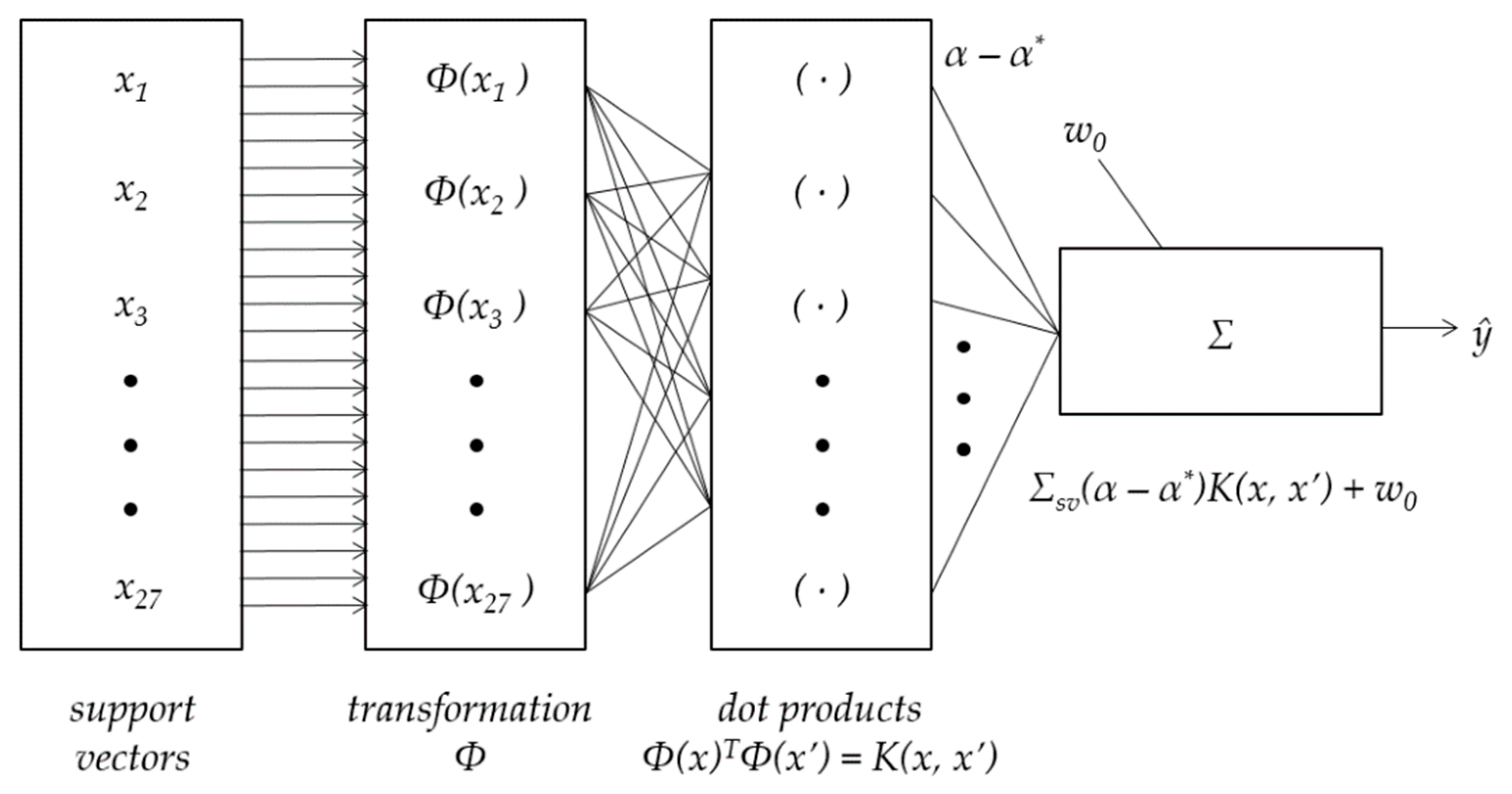
The following fundamentals of the method were compiled and summarized after [17,18,19,20,21]. The SVM method allows approximating f as a linear hyperplane. The linear approximation is achieved specifically for nonlinear problems due to a transformation of independent variable space to a higher dimensional, linear feature space. If the set of training examples is given as χ such that: { χ = [x, y] ∈ Rm × R } and Φ is a nonlinear transformation used to determine a new feature space H for the inputs: Φ: Rm → H, Φ(x) ∈ H, y ∈ R, then the function f can be given as follows:
f(x) = wTΦ(x) + w0
The transformation Φ(x) is supposed to increase the expressive power of the representation, and the approximation function is computed in the higher dimensional, linear feature space H. Support vectors (sv) are the training data points that lie closest to the hyperplane and thus they affect its optimal location.
To measure the errors of the training process, Vapnik’s ε-insensitive loss function is assumed:
where:
l(f(x),y) = |y − f(x)|ε,
|y − f(x)|ε = 0 for |y − f(x)| ≤ ε and |y − f(x)|ε = |y − f(x) | − ε for |y − f(x)| > ε,
Here, ε defines a tube of insensitiveness used to fit the training examples around the true values y.
In other words, the value of ε affects the number of support vectors.
Following this the, problem comes down to optimization by machine learning:
subject to the constraints for the both sides of ε-tube:
½ǁwǁ2 + CΣ(ξ − ξ*) → min,
wTΦ(x) + w0 − y ≤ ε + ξ and y − (wTΦ(x) + w0) ≤ ε + ξ* and ξ, ξ* ≥ 0
The use of loss function (3) results in toleration of deviations smaller than ε. The C represents the regularization parameter in the SVM method, and determines a compromise between decision function’s margin against training accuracy. It determines the compromise between the complexity of a model and ξ, and ξ* in (5) and (6) are slack variables that penalize predictions out of the ε-tube. The optimization of (5) is solved with the use of Lagrange multipliers:
where nsv stands for the number of support vectors and α, α* are the multipliers for the optimal solution such as:
f(x) = Σnsv(α − α*)Φ(x)TΦ(x′) + w0,
0 ≤ α ≤ C and 0 ≤ α ≤ C
The choice of appropriate transformation Φ and explicit calculation of Φ(x)TΦ(x′) is difficult and computationally complex. To simplify the computations, the kernel functions K(x, x′) are introduced instead:
K(x, x′) = Φ(x)TΦ(x′),
The kernel functions which are mostly mentioned for the use in the SVM method are: polynomial (10), radial basis (11), and sigmoidal (12):
K(x, x′) = tanh(γx·x′ + c),
K(x, x′) = exp(− γǁx − x′ǁ2),
K(x, x′) = (γx·x′ + c)d,
Taking into account the above, the approximation function can be given finally as:
f(x) = Σsv(α − α*)K(x, x′) + w0,
2.2. Variables of the Model and the Concept of Model Development
Before the start of actual regression analysis, data that reflected the values of model variables were collected and analyzed. The collected data included information about road bridges, rail bridges, and animal bridges (as wildlife crossings) built in Poland between 2005 and 2018. In terms of total construction costs, the real-life values were updated to be comparable—regardless of the date of project completion—with the use of price indices of construction assembly production published by the General Statistical Office in Poland. Later in the paper, the updated costs of bridges given in millions of PLN (e.g., PLN 10.53 m) are referred to as y. For better recognition, the costs are given in millions of EUR as well (e.g., EUR 2.45 m). The conversion was made on the basis of the Polish National Bank official exchange rate for the PLN/EUR pair of currencies published for 31.12.2018. The values of y varied between PLN 2.46 m (EUR 0.57 m) and PLN 23.48 m (EUR 5.46 m).
The cost predictors, as the independent variables, brought to the model information about the type of bridge, type of project, structural and material solutions, types of supports and their foundations, and load class. All the mentioned information was initially recorded as nominal data. Moreover, basic size measures, in terms of the decks’ total length and width, as well as the number of spans, were taken into account. The independent variables of a model are presented in Table 1. In this table, one can see that finally the characteristics of bridges recorded initially as nominal data were coded as binary values (0 or 1). Information recorded as numerical data was scaled to the range <0; 1>. In the case of structural solution, type of intermediate supports and load class, the values for x14, x22, and x27 were introduced to represent more than one nominal value that were ARCHED/BOX, COLUMNS/PILES, and k/C/D/E, respectively (see also the footnotes under Table 1). This was done due to the fact that some nominal values were not numerous enough in the dataset to be represented alone by one binary variable. It is important to note that for each of the characteristics listed in Table 1, only one nominal value was allowed, so only one of the binary variables belonging to this characteristic could take value 1. For example, for the type of a structure of which the nominal value was VIADUCT, the values x1 − x3 equaled x1 = 0, x2 = 1, x3 = 0.
Table 2 presents a random sample of the coded variables x and y as used for model development, and p stands for pattern number.
The selection of the cost predictors was based on the availability of information in the early stages of the bridge construction projects. The characteristics and their values that became independent variables of the model (as presented in Table 1) can be easily identified in at beginning of the design process.
Overall, the number of patterns to be used for the process of machine learning and testing models equaled 167. The data was collected from the public clients responsible for bridge construction projects in Poland. The data was divided into two subsets—the first subset (later denoted as L) was used for the machine learning purposes, the second subset (later denoted as T) was used for the models’ testing purposes. Both subsets were selected so as to be equivalent and to ensure their representativeness in terms of the features of the investigated bridges and the range of construction costs as well. The cardinality of subset L equaled 131, whereas the cardinality of subset T equaled 36. One can easily note that the number of patterns belonging to subset T accounted for more than 20% of the overall number of collected data patterns.
The research included an investigation of the number of SVM-based regression models. A schematic diagram of the investigated models is presented in Figure 1.
The SVM-based models’ performance rely on the assumed kernel function and its parameters as well as C and ε meta-parameters.
For the purposes of transformation Φ, the use of the three aforementioned kernel functions (10)–(12) were investigated, however the best results were obtained for radial basis function (11). Thus, in the two following sections, the author focused on a presentation and discussion of the models in which this particular type of function was applied.
- The choice is made on the basis of the a priori knowledge of the problem and/or users’ expertise;
- Values are selected on the basis of the grid search;
- Determination of the parameters directly from the data;
- Assuming C equal to the range of output values;
- Tuning ε parameter to the training data noise density.
The choice of the two parameters for the models proposed herein compromised the above-mentioned approaches, namely determination of the parameters on the basis of the training data and grid search.
Each of the models was analyzed and its predictive performance was assessed in terms of correlation between the real-life values of the bridges’ total construction costs y and the predicted values ŷ, the predictions’ errors, and the residuals analysis. The following equations were used for computations of Pearson’s correlation coefficient (R), root mean squared error (RMSE), mean absolute percentage error (MAPE), and absolute percentage error for p-th case (APEp):
where cov(y;ŷ)—covariance of real values of the bridges’ total construction costs and values predicted by a model, σy and σŷ standard deviations of real values of the bridges total construction costs and values predicted by a model, respectively; n—cardinality of either L or T subset, y − ŷ—prediction errors, computed after completion of the machine learning process for either L or T subset; and p—pattern index. The SVM machine learning process was made with the use of STATISTICATM software suite.
R = cov(y;ŷ)/(σyσŷ),
RMSE = (1/n·Σ(y − ŷ)2)0.5,
MAPE = 1/100%·Σ[(|y − ŷ|)/y],
APEp = 100%· (|yp − ŷp|)/yp,
According to the literature [36,37,38] and remarks about the expected accuracy of cost estimates provided at the early stages of construction projects (also called conceptual estimates), the error of estimates should fall into the ranges <−30%/−25% and +25%/+30%> when compared to the actual, final construction costs. If the proposed models’ predictions and APEp are considered, the above rule can be reformulated into the expectation about the desired range of APEp between 0% and +25%/+30%. What is obvious is that the predictions of the bridges’ total construction costs are still required to be provided by the models with errors as small as possible. However, the rule can be used for the purposes of the models’ performance comparison and assessment.
3. Results
For the investigated SVM-based regression models, the parameter γ (for radial basis kernel function) was assumed as the inverse of the number of inputs, thus γ = 1/27 = 0.037. The γ value can be explained as the inverse of the radius of influence of samples selected in the course of machine learning to be support vectors.
Regularization meta-parameter C was initially assessed following the rule [35]:
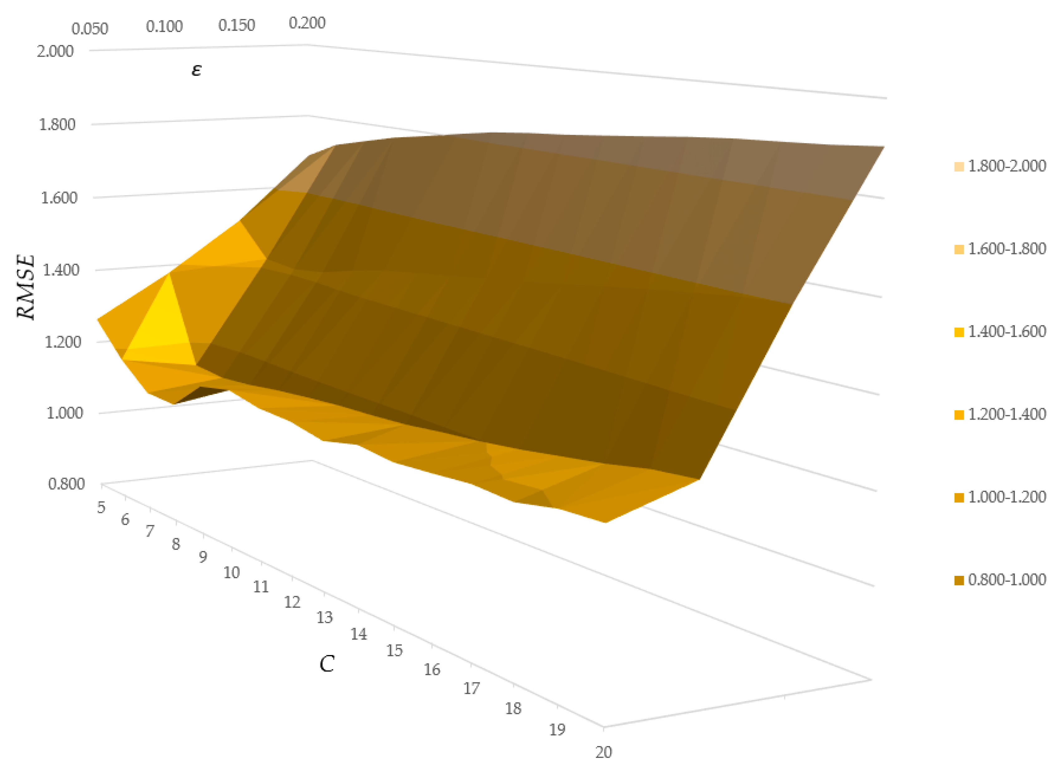
where E(y) = 6.61 and σy = 4.22 computed for yp belonging to subset L resulted in C = 19.27. After this, it was assumed that 20 will constitute the upper boundary of C. Values of C were sought for with the use of grid search; the values of ε (threshold of the loss function) were also sought for with the use of grid search. The considered ranges of C and ε, as well as the grid search details, are given in Table 3.
C = max{|E(y) + 3σy|; |E(y) − 3σy|},
The machine learning process for each of the models was carried out with the use of 10-fold cross-validation. Having finished the process, the performances of the models were compared. RMSE values were computed for both L and T subsets for all of the obtained models. The RMSE values obtained for the subset that was used in the course of machine learning (subset L) are presented in Figure 2. Figure 3 depicts RMSE values computed for testing subset T. The values of errors (height axes in Figure 2 and Figure 3) are presented as 3D surfaces with regard to C (length axes) and ε (depth axes). One can see that in the case of RMSE, the values computed for subset L are decreasing with the increase of C and decrease of ε. On the other hand, the tendency for errors computed for subset T is similar with regards to ε, however the opposite with regard to C.
When considering the values of RMSE for both subsets L and T together, one can find the points in the grid representing errors of learning and testing computed for certain models, where the values of RMSE for testing reach minimums; moreover, the values of RMSE for machine learning are close.
The analysis of RMSE values allowed for the selection of five models that were further investigated. The five bridges’ construction cost prediction models based on support vector regression (later referred to as BCCPMSVR) are introduced in Table 4. Characteristics of the models include values of meta-parameters C and ε, number of support vectors (sv), and number of bounded support vectors and values of the constants w0. The support vectors are the data patterns belonging to subset L that determine the position of the regression hyperplane for a certain model. Furthermore, errors of 10-fold cross-validation are also presented. General error and performance measures RMSE, R, and MAPE for the five BCCPMSVR models, computed for L and T subsets, are set together in Table 5.
The values of RMSE and R (in Table 5), when comparing the five selected models, are relatively close. Thus, in light of the RMSE and R values analysis, the performance of the models can be assessed as comparable. In terms of MAPE values, the differences are slightly more evident. The final choice of the model, however, was based on the comparison of the distribution of APEp errors and the rule, (presented in Section 2.2) that refers to the desired range of APEp values for bridge construction early cost estimates.
Table 6 presents the distributions of APEp errors of predictions of total bridge construction costs both for L and T subsets under the conditions that APEp ≤ 25% or APEp ≤ 30%. In light of the analysis of the values in Table 6, model BCCPMSVR 2 was proven to perform better than the others—the model reached the highest shares of APEp ≤ 25% for L and T subsets and the same shares of APEp ≤ 30% for L and T subsets as BCCPMSVR1.
For the finally selected model of BCCPMSVR2, the scatter plots of values of y (actual bridge construction costs, presented on the horizontal axes) and ŷ (bridge construction cost predictions by model BCCPMSVR 2, presented on the vertical axes) are depicted in Figure 4 and Figure 5. The former shows the scatter plot of y and ŷ values for subset L, the latter for subset T. The charts include also the cones of errors ±25% and ±30%.
Table 7 presents the percentage shares of APEp errors of bridge construction cost predictions provided by the model BCCPMSVR2 (both for L and T subsets) divided into intervals of a range equal to 5%. Additionally, distributions (cumulated shares) of APEp errors are given in the Table.
The distribution of points (yp; ŷp) in the scatter plots (in Figure 4 and Figure 5) is even along the line of a perfect fit. Moreover, for both of the subsets L and T, the vast majority of bridge construction cost predictions are located within the ±25% cone of errors; almost all of the predictions are located within the ±30% cone of errors.
The values of the APEp, (in Table 6), as complementary information, confirm that most of the bridge construction cost predictions made by BCCPMSVR2 meet the condition of early cost estimates.
The general conclusion on the results presented above is that the proposed model provides the predictions of costs for bridge construction projects with satisfactory accuracy regarding the expectations for estimates at the early stages of projects.
4. Discussion
When compared to the models proposed by other authors, some significant differences of the model introduced herein can be indicated. The previous works that aimed at modeling costs of bridges in the early stages of projects were focused on cost estimates of either parts of bridge structures [2,3,4] or specific types of bridges [5,6,7,8]. The model introduced herein offers cost predictions of bridges as a whole object (the substructure and superstructure together). Moreover, the predictions are made for different types of bridges with regard to their structure, purpose, and structural and material solutions.
On the other hand, most of the previously proposed models are based either on regression analysis [2,3,4] or ANN [5]. The former requires a priori assumptions about the functional relationship binding bridge construction cost as a dependent variable with cost predictors as independent variables. The latter are at risk of the so-called local minima problem. Both of these drawbacks are overcome by the use of the SVM-based regression method for the development of the model for prediction costs of bridges.
The results of the research confirmed the assumptions made for the application of the SVM method for bridge construction cost prediction. Several SVM-based regression models were investigated with the use of data collected for a number of bridge construction projects completed in Poland. Having finished machine learning and testing processes, five of the models, of satisfactory knowledge generalization ability and comparable performance, were preselected. An important fact to be mentioned here is that in the case of repetitions of machine learning processes with given constraints, the results obtained for each of the investigated models were exactly the same every time. Application of the SVM method for early estimates of bridge construction costs eliminates the risks of local minima problem.
The final selection of the best model was based on the comparison and analysis ability to predict the bridge construction costs with accuracy appropriate for the early stage of the projects.
The general performance of the selected model, namely BCCPMSVR2, and its measures are presented in Section 3. The predictions of the bridge construction costs provided by the model can also be analyzed in a way that focuses on selected characteristics and features of bridges as the model’s input.
Table 8, Table 9, Table 10 and Table 11 present relative percentage shares of APEp, computed for the machine learning subset, belonging to certain intervals (compare Table 7) with regard to variables of a nominal type (coded as binary values for machine learning). The relative percentage shares of APEp for variables of nominal type were computed as follows:
- For each of the variables xj for j = 1 − 8 or j = 12 − 27, the number of predictions that fulfilled the condition of having corresponding APEp that fell into the certain interval were counted and divided by the number of occurrences of xj = 1.
Analyzing the Table 8, Table 9, Table 10 and Table 11, one can see how the predictions accuracy depends relatively on the certain, chosen characteristics of the bridges described by the nominal values.
Table 12, Table 13 and Table 14 present the relative percentage shares of APEp, computed for the machine learning subset, belonging to certain intervals (compare Table 6) with regard to variables of a numerical type.
The relative percentage shares of APEp for these variables were computed as follows: for each of the variables xj for j = 9 − 11:
- Predictions for variables values that fulfilled the conditions of falling into certain range of values and having corresponding APEp from a certain error’s interval were counted and divided by the number of occurrences.
Analyzing the Table 12, Table 13 and Table 14 one can see how the predictions accuracy depends relatively on the certain, chosen characteristics of the bridges described by the structure’s length, width or number of spans.
A limitation of the model that should be mentioned here is that the real-life bridge construction costs were updated for a certain moment in time for the data that was used both in the machine learning and in the testing processes. Thus, for now, dynamical predictions are not provided by the developed model. The reason for this limitation is the number of collected data patterns which does not currently allow for dynamical predictions that comply to the changes of costs in time.
Future research plans cover the issue of database expansion and further collection of training data, and development of models capable of dynamical predictions. One of the possible future research directions, which also rely on the database expansion, is the decomposition of the problem, development of separate models for certain types of bridges and combining the models in a so-called committee machine.
5. Conclusions
As a result of the research, an original model capable of supporting early estimates of bridge construction costs, based on machine learning and SVM method, was developed and introduced. The input variables bring to the model information, available in the early stage of a bridge construction project, that represent the features of bridges.
According to the presented results and discussion, as well as the accuracy expectations applicable for conceptual estimates, the model offers good performance. Applied kernel functions are of the radial basis type, and the meta-parameters of the model are C = 8 and ε = 0.050. The values of the general measures of the model’s performance, respectively for machine learning and testing, are:
- RMSE: 1.058 and 1.111;
- Pearson’s correlation coefficient R of real-life bridge construction costs and costs predicted by the model: 0.974 and 0.980;
- MAPE: 13.85% and 10.94%.
The model provides cost predictions with satisfactory accuracy, within the range of errors appropriate for early estimates (conceptual estimates) that is ±25%/30%.
The proposed approach is prospective for early cost estimates (conceptual cost estimates) in bridge construction projects. The study contributes to the body of knowledge by the application of machine learning methods for cost analyses in construction.
Funding
This research was funded by statutory activities of Cracow University of Technology.
Acknowledgments
Computations for SVM machine learning were done with the use of STATISTICATM software suite.
Conflicts of Interest
The author declares no conflicts of interest.
References
- Hollar, D.A.; Rasdorf, W.; Liu, M.; Hummer, J.E.; Arocho, I.; Hsiang, S.M. Preliminary engineering cost estimation model for bridge projects. J. Constr. Eng. Manag. 2012, 139, 1259–1267. [Google Scholar] [CrossRef]
- Fragkakis, N.; Lambropoulos, S.; Tsiambaos, G. Parametric model for conceptual cost estimation of concrete bridge foundations. J. Infrastruct. Syst. 2010, 17, 66–74. [Google Scholar] [CrossRef]
- Alhusni, M.K.; Triwiyono, A.; Irawati, I.S. Material quantity estimation modelling of bridge sub-substructure using regression analysis. MATEC Web Conf. 2019, 258, 02008. [Google Scholar] [CrossRef]
- Fragkakis, N.; Lambropoulos, S.; Pantouvakis, J.P. A cost estimate method for bridge superstructures using regression analysis and bootstrap. Org. Technol. Manag. Constr. Int. J. 2010, 2, 182–190. [Google Scholar]
- Creese, R.C.; Li, L. Cost estimation of timber bridges using neural networks. Cost Eng. 1995, 37, 17–22. [Google Scholar]
- Kim, K.J.; Kim, K.; Kang, C.S. Approximate cost estimating model for PSC Beam bridge based on quantity of standard work. KSCE J. Civ. Eng. 2009, 13, 377–388. [Google Scholar] [CrossRef]
- Kim, B.S. The approximate cost estimating model for railway bridge project in the planning phase using CBR method. KSCE J. Civ. Eng. 2011, 15, 1149–1159. [Google Scholar] [CrossRef]
- Fragkakis, N.; Lambropoulos, S.; Pantouvakis, J.P. A computer-aided conceptual cost estimating system for pre-stressed concrete road bridges. Int. J. Inf. Technol. Proj. Manag. 2014, 5, 1–13. [Google Scholar] [CrossRef] [Green Version]
- Marzouk, M.; Hisham, M. Applications of building information modeling in cost estimation of infrastructure bridges. Int. J. 3-D Inf. Model. 2012, 1, 17–29. [Google Scholar] [CrossRef]
- Choudhry, R.M.; Aslam, M.A.; Hinze, J.W.; Arain, F.M. Cost and schedule risk analysis of bridge construction in Pakistan: Establishing risk guidelines. J. Constr. Eng. Manag. 2014, 140, 04014020. [Google Scholar] [CrossRef]
- Saito, M.; Sinha, K.C.; Anderson, V.L. Statistical models for the estimation of bridge replacement costs. Transp. Res. Part A Gen. 1991, 25, 339–350. [Google Scholar] [CrossRef]
- Bouabaz, M.; Hamami, M. A cost estimation model for repair bridges based on artificial neural network. Am. J. Appl. Sci. 2008, 5, 334–339. [Google Scholar] [CrossRef] [Green Version]
- Chengalur-Smith, I.N.; Ballou, D.P.; Pazer, H.L. Modeling the costs of bridge rehabilitation. Transp. Res. Part A Policy Pract. 1997, 31, 281–293. [Google Scholar] [CrossRef]
- Padgett, J.; DesRoches, R.; Nielson, B.; Yashinsky, M.; Kwon, O.S.; Burdette, N.; Tavera, E. Bridge damage and repair costs from Hurricane Katrina. J. Bridge Eng. 2008, 13, 6–14. [Google Scholar] [CrossRef] [Green Version]
- Ehlen, M.A. Life-cycle costs of fiber-reinforced-polymer bridge decks. J. Mater. Civ. Eng. 1999, 11, 224–230. [Google Scholar] [CrossRef]
- Hassanain, M.A.; Loov, R.E. Cost optimization of concrete bridge infrastructure. Can. J. Civ. Eng. 2003, 30, 841–849. [Google Scholar] [CrossRef]
- Vapnik, V. Statistical Learning Theory; John Wiley & Sons: New York, NY, USA, 1998. [Google Scholar]
- Vapnik, V. The Nature of Statistical Learning Theory; Springer: New York, NY, USA, 2013. [Google Scholar]
- Smola, A.J.; Schölkopf, B. A tutorial on support vector regression. Stat. Comput. 2004, 14, 199–222. [Google Scholar] [CrossRef] [Green Version]
- Cristianini, N.; Shawe-Taylor, J. An Introduction to Support Vector Machines (and Other Kernel-based Learning Methods); Cambridge University Press: Cambridge, UK, 2000. [Google Scholar]
- Gunn, S.R. Support Vector Machines for Classification and Regression; Technical Report; University of Southampton: Southampton, UK, 1998. [Google Scholar]
- Caldas, C.H.; Soibelman, L. Automating hierarchical document classification for construction management information systems. Autom. Constr. 2003, 12, 395–406. [Google Scholar] [CrossRef]
- Mahfouz, T.; Kandil, A. Construction legal decision support using support vector machine (SVM). In Proceedings of the Construction Research Congress 2010: Innovation for Reshaping Construction Practice, Banff, AB, Canada, 8–10 May 2010; pp. 879–888. [Google Scholar] [CrossRef]
- Chen, J.H.; Lin, J.Z. Developing an SVM based risk hedging prediction model for construction material suppliers. Autom. Constr. 2010, 19, 702–708. [Google Scholar] [CrossRef]
- Tserng, H.P.; Lin, G.F.; Tsai, L.K.; Chen, P.C. An enforced support vector machine model for construction contractor default prediction. Autom. Constr. 2011, 20, 1242–1249. [Google Scholar] [CrossRef]
- Horta, I.M.; Camanho, A.S. Company failure prediction in the construction industry. Expert Syst. Appl. 2013, 40, 6253–6257. [Google Scholar] [CrossRef]
- Cheng, M.Y.; Wu, Y.W.; Wu, C.F. Project success prediction using an evolutionary support vector machine inference model. Autom. Constr. 2010, 19, 302–307. [Google Scholar] [CrossRef]
- Cheng, M.Y.; Hoang, N.D.; Wu, Y.W. Hybrid intelligence approach based on LS-SVM and Differential Evolution for construction cost index estimation: A Taiwan case study. Autom. Constr. 2013, 35, 306–313. [Google Scholar] [CrossRef]
- Wang, Y.R.; Yu, C.Y.; Chan, H.H. Predicting construction cost and schedule success using artificial neural networks ensemble and support vector machines classification models. Int. J. Proj. Manag. 2012, 30, 470–478. [Google Scholar] [CrossRef]
- Cheng, M.Y.; Hoang, N.D. Interval estimation of construction cost at completion using least squares support vector machine. J. Civ. Eng. Manag. 2014, 20, 223–236. [Google Scholar] [CrossRef]
- Kim, G.-H.; Shin, J.-M.; Kim, S.; Shin, Y. Comparison of School Building Construction Costs Estimation Methods Using Regression Analysis, Neural Network and Support Vector Machine. J. Build. Constr. Plan. Res. 2013, 1, 1–7. [Google Scholar] [CrossRef] [Green Version]
- Peško, I.; Mučenski, V.; Šešlija, M.; Radović, N.; Vujkov, A.; Bibić, D.; Krklješ, M. Estimation of Costs and Durations of Construction of Urban Roads Using ANN and SVM. Complexity 2017, 2017, 2450370. [Google Scholar] [CrossRef] [Green Version]
- Scholkopf, B.; Burges, J.; Smola, A. Advances in Kernel Methods: Support Vector Learning; MIT Press: Cambridge, MA, USA, 1998. [Google Scholar]
- Cherkassky, V.; Mulier, F. Learning from Data. Concepts, Theory, and Methods: Second Edition; John Wiley & Sons: Hoboken, NJ, USA, 2006. [Google Scholar] [CrossRef]
- Cherkassky, V.; Ma, Y. Practical selection of SVM parameters and noise estimation for SVM regression. Neural Netw. 2004, 17, 113–126. [Google Scholar] [CrossRef] [Green Version]
- Brook, M. Estimating and Tendering for Construction Work; Routledge: Abingdon, UK, 2016. [Google Scholar] [CrossRef]
- Kasprowicz, T. Inżynieria Przedsięwzięć Budowlanych in KAPLIŃSKI O; Metody i modele badań w inżynierii przedsięwzięć budowlanych; PAN KILIW: Warszawa, 2007; pp. 35–78. [Google Scholar]
- Potts, K. Construction Cost Management: Learning from Case Studie; Taylor & Francis: Abingdon, UK, 2008. [Google Scholar]
Figure 1.
Schematic diagram of the investigated support vector machine (SVM)-based regression models.
Figure 1.
Schematic diagram of the investigated support vector machine (SVM)-based regression models.

Figure 2.
RMSE errors obtained for subset L.

Figure 3.
RMSE errors computed for subset T.

Figure 4.
Scatter plot of y and ŷ predicted by BCCPMSVR2 for subset L.

Figure 5.
Scatter plot of y and ŷ predicted by BCCPMSVR2 for subset T.


Table 1.
Input data for regression model—independent variables.
| Characteristic | Nominal Values | Coding | Symbol |
|---|---|---|---|
| Type of a structure | BRIDGE | binary | x1 |
| VIADUCT | binary | x2 | |
| WHARF | binary | x3 | |
| Type of a bridge | ROAD BRIDGE | binary | x4 |
| RAIL BRIDGE | binary | x5 | |
| ANIMAL BRIDGE | binary | x6 | |
| Type of a project | BUILD | binary | x7 |
| DESIGN&BUILD | binary | x8 | |
| Total length | LENGTH [m] | numerical | x9 |
| Width of a structure | WIDTH [m] | numerical | x10 |
| Number of spans | SPANS | numerical | x11 |
| Structural solution | BEAM | binary | x12 |
| FRAME | binary | x13 | |
| ARCHED/BOX | binary | x14 | |
| Material solution | REINFORCED CONCRETE | binary | x15 |
| PRESTRESSED CONCRETE | binary | x16 | |
| STEEL | binary | x17 | |
| Bridgehead supports | SOLID-WALLED | binary | x18 |
| COLUMNS | binary | x19 | |
| Intermediate supports | NONE | binary | x20 |
| SOLID-WALLED | binary | x21 | |
| COLUMNS/PILES | binary | x22 | |
| Supports’ foundations | SHALLOW | binary | x23 |
| DEEP | binary | x24 | |
| Load class * | A | binary | x25 |
| B | binary | x26 | |
| k/C/D/E 1 | binary | x27 |
1 k for rail bridges or C, D, E for other bridges; * according to standards applied in Poland.
Table 2.
Random sample of the model’s variable values.
| p | 10 | 77 | 83 | 104 | 109 | 111 | 119 | 150 | 166 |
|---|---|---|---|---|---|---|---|---|---|
| x1 | 1 | 0 | 0 | 0 | 1 | 0 | 1 | 0 | 0 |
| x2 | 0 | 1 | 1 | 0 | 0 | 1 | 0 | 1 | 0 |
| x3 | 0 | 0 | 0 | 1 | 0 | 0 | 0 | 0 | 1 |
| x4 | 0 | 0 | 0 | 0 | 0 | 1 | 1 | 0 | 0 |
| x5 | 0 | 1 | 1 | 1 | 0 | 0 | 0 | 0 | 1 |
| x6 | 1 | 0 | 0 | 0 | 1 | 0 | 0 | 1 | 0 |
| x7 | 1 | 1 | 1 | 1 | 1 | 0 | 0 | 1 | 0 |
| x8 | 0 | 0 | 0 | 0 | 0 | 1 | 1 | 0 | 1 |
| x9 | 0.069 | 0.151 | 0.150 | 0.219 | 0.197 | 0.180 | 0.456 | 0.095 | 0.715 |
| x10 | 0.114 | 0.057 | 0.027 | 0.114 | 0.114 | 0.092 | 0.097 | 0.426 | 0.049 |
| x11 | 0.000 | 0.000 | 0.143 | 0.143 | 0.143 | 0.000 | 0.286 | 0.071 | 0.500 |
| x12 | 1 | 1 | 0 | 1 | 1 | 0 | 0 | 0 | 1 |
| x13 | 0 | 0 | 1 | 0 | 0 | 0 | 0 | 1 | 0 |
| x14 | 0 | 0 | 0 | 0 | 0 | 1 | 1 | 0 | 0 |
| x15 | 0 | 0 | 1 | 0 | 0 | 0 | 1 | 0 | 0 |
| x16 | 1 | 1 | 0 | 1 | 0 | 0 | 0 | 1 | 1 |
| x17 | 0 | 0 | 0 | 0 | 1 | 1 | 0 | 0 | 0 |
| x18 | 1 | 0 | 1 | 1 | 1 | 1 | 1 | 1 | 1 |
| x19 | 0 | 1 | 0 | 0 | 0 | 0 | 0 | 0 | 0 |
| x20 | 0 | 0 | 1 | 0 | 1 | 0 | 0 | 0 | 0 |
| x21 | 0 | 0 | 0 | 1 | 0 | 0 | 1 | 1 | 1 |
| x22 | 1 | 1 | 0 | 0 | 0 | 1 | 0 | 0 | 0 |
| x23 | 0 | 1 | 0 | 1 | 0 | 1 | 0 | 1 | 0 |
| x24 | 1 | 0 | 1 | 0 | 1 | 0 | 1 | 0 | 1 |
| x25 | 1 | 0 | 0 | 1 | 1 | 0 | 0 | 0 | 0 |
| x26 | 0 | 1 | 1 | 0 | 0 | 0 | 0 | 0 | 1 |
| x27 | 0 | 0 | 0 | 0 | 0 | 1 | 1 | 1 | 0 |
| y [PLN] | 3.02 | 5.49 | 6.11 | 9.84 | 10.82 | 12.54 | 14.15 | 6.83 | 19.85 |
| y [EUR] 1 | 0.70 | 1.28 | 1.42 | 2.29 | 2.52 | 2.92 | 3.29 | 1.59 | 4.62 |
1 training and testing of the model was done with the use of costs given in millions of PLN.
Table 3.
Considered ranges of length axis (C) and depth axes (ε) parameters.
| Parameter | Lower Boundary | Step | Upper Boundary |
|---|---|---|---|
| C | 5 | 1 | 20 |
| ε | 0.05 | 0.05 | 0.20 |
Table 4.
Five selected models and their characteristics.
| Model | C | ε | sv | Bounded sv | w0 | Cross-Validation Error |
|---|---|---|---|---|---|---|
| BCCPMSVR1 | 7 | 0.050 | 91 | 50 | −0.108761 | 0.038 |
| BCCPMSVR2 | 8 | 0.050 | 85 | 47 | −0.118497 | 0.037 |
| BCCPMSVR3 | 8 | 0.100 | 59 | 24 | −0.132814 | 0.037 |
| BCCPMSVR4 | 9 | 0.100 | 58 | 23 | −0.137849 | 0.036 |
| BCCPMSVR5 | 10 | 0.100 | 56 | 22 | −0.130312 | 0.035 |
Table 5.
Measures of errors and performance obtained for the five selected models.
| Model | RMSEL | RMSET | RL | RT | MAPEL | MAPET |
|---|---|---|---|---|---|---|
| BCCPMSVR1 | 1.115 | 1.112 | 0.971 | 0.979 | 14.64% | 11.33% |
| BCCPMSVR2 | 1.058 | 1.111 | 0.974 | 0.980 | 13.85% | 10.94% |
| BCCPMSVR3 | 1.175 | 1.141 | 0.968 | 0.978 | 17.03% | 11.44% |
| BCCPMSVR4 | 1.139 | 1.152 | 0.970 | 0.978 | 16.69% | 11.28% |
| BCCPMSVR5 | 1.115 | 1.161 | 0.971 | 0.978 | 16.56% | 11.30% |
Table 6.
Comparison of absolute percentage error for p-th case (APEp) errors for the five selected models.
Table 6.
Comparison of absolute percentage error for p-th case (APEp) errors for the five selected models.
| Subset L | Subset T | |||
|---|---|---|---|---|
| Model | APEp ≤ 25% | APEp ≤ 30% | APEp ≤ 25% | APEp ≤ 30% |
| BCCPMSVR1 | 85.38% | 92.31% | 81.08% | 91.89% |
| BCCPMSVR2 | 86.92% | 92.31% | 83.78% | 91.89% |
| BCCPMSVR3 | 72.31% | 80.00% | 81.08% | 89.19% |
| BCCPMSVR4 | 73.08% | 80.77% | 81.08% | 89.19% |
| BCCPMSVR5 | 73.85% | 82.31% | 83.78% | 89.19% |
Table 7.
Shares and distribution of APEp values for BCCPMSVR2.
| Subset | Subset | ||||
|---|---|---|---|---|---|
| Share | L | T | Distribution | L | T |
| APEp ≤ 5% | 20.77% | 27.03% | APEp ≤ 5% | 20.77% | 27.03% |
| 5% < APEp ≤ 10% | 20.77% | 37.84% | APEp ≤ 10% | 41.54% | 64.86% |
| 10% < APEp ≤ 15% | 24.62% | 10.81% | APEp ≤ 15% | 66.15% | 75.68% |
| 15% < APEp ≤ 20% | 10.77% | 5.41% | APEp ≤ 20% | 76.92% | 81.08% |
| 20% < APEp ≤ 25% | 10.00% | 2.70% | APEp ≤ 25% | 86.92% | 83.78% |
| 25% < APEp ≤ 30% | 5.38% | 8.11% | APEp ≤ 30% | 92.31% | 91.89% |
| APEp > 30% | 7.69% | 8.11% | APEp > 30% | 100.00% | 100.00% |
Table 8.
APEp predictions’ errors for machine learning with regard to the type of bridge its structure and type of a project.
Table 8.
APEp predictions’ errors for machine learning with regard to the type of bridge its structure and type of a project.
| Relative Percentage Share of APEp | |||||||
|---|---|---|---|---|---|---|---|
| 0–5% | 5–10% | 10–15% | 15–20% | 20–25% | 25–30% | >30% | |
| BRIDGE (x1) | 35.71% | 14.29% | 14.29% | 7.14% | 7.14% | 14.29% | 7.14% |
| VIADUCT (x2) | 15.31% | 21.43% | 28.57% | 12.24% | 11.22% | 3.06% | 8.16% |
| WHARF (x3) | 60.00% | 40.00% | 0.00% | 0.00% | 0.00% | 0.00% | 0.00% |
| ROAD BRIDGE (x4) | 17.65% | 11.76% | 26.47% | 8.82% | 14.71% | 5.88% | 14.71% |
| RAIL BRIDGE (x5) | 18.39% | 25.29% | 25.29% | 10.34% | 9.20% | 5.75% | 5.75% |
| ANIMAL BRIDGE (x6) | 60.00% | 10.00% | 10.00% | 20.00% | 0.00% | 0.00% | 0.00% |
| BUILD (x7) | 15.65% | 22.61% | 26.96% | 11.30% | 10.43% | 6.09% | 6.96% |
| DESIGN&BUILD (x8) | 62.50% | 6.25% | 6.25% | 6.25% | 6.25% | 0.00% | 12.50% |
Table 9.
APEp predictions’ errors for machine learning with regard to the structural and material solutions.
Table 9.
APEp predictions’ errors for machine learning with regard to the structural and material solutions.
| Relative Percentage Share of APEp | |||||||
|---|---|---|---|---|---|---|---|
| 0–5% | 5–10% | 10–15% | 15–20% | 20–25% | 25–30% | >30% | |
| BEAM (x12) | 19.64% | 20.54% | 26.79% | 9.82% | 8.93% | 5.36% | 8.93% |
| FRAME (x13) | 15.31% | 21.43% | 28.57% | 12.24% | 11.22% | 3.06% | 8.16% |
| ARCHED/BOX (x14) | 54.55% | 9.09% | 9.09% | 9.09% | 9.09% | 9.09% | 0.00% |
| REINFORCED CONCRETE (x15) | 18.33% | 15.00% | 26.67% | 8.33% | 15.00% | 5.00% | 11.67% |
| PRESTRESSED CONCRETE (x16) | 20.83% | 29.17% | 25.00% | 8.33% | 6.25% | 6.25% | 4.17% |
| STEEL (x17) | 30.43% | 17.39% | 17.39% | 21.74% | 4.35% | 4.35% | 4.35% |
Table 10.
APEp predictions’ errors for machine learning with regard to the types of bridgehead and intermediate supports and supports’ foundations.
Table 10.
APEp predictions’ errors for machine learning with regard to the types of bridgehead and intermediate supports and supports’ foundations.
| Relative Percentage Share of APEp | |||||||
|---|---|---|---|---|---|---|---|
| 0–5% | 5–10% | 10–15% | 15–20% | 20–25% | 25–30% | >30% | |
| SOLLID-WALLED (x18) | 21.77% | 20.16% | 23.39% | 10.48% | 10.48% | 5.65% | 8.06% |
| COLUMNS (x19) | 14.29% | 28.57% | 42.86% | 14.29% | 0.00% | 0.00% | 0.00% |
| NONE (x20) | 11.11% | 14.29% | 34.92% | 12.70% | 11.11% | 6.35% | 9.52% |
| SOLLID-WALLED (x21) | 36.36% | 18.18% | 22.73% | 9.09% | 9.09% | 0.00% | 4.55% |
| COLUMNS/PILES (x22) | 28.26% | 30.43% | 10.87% | 8.70% | 8.70% | 6.52% | 6.52% |
| SHALLOW (x23) | 12.68% | 22.54% | 30.99% | 7.04% | 14.08% | 5.63% | 7.04% |
| DEEP (x24) | 31.67% | 18.33% | 16.67% | 15.00% | 5.00% | 5.00% | 8.33% |
Table 11.
APEp predictions’ errors for machine learning with regard to the load class.
| Relative Percentage Share of APEp | |||||||
|---|---|---|---|---|---|---|---|
| 0–5% | 5–10% | 10–15% | 15–20% | 20–25% | 25–30% | >30% | |
| A (x25) | 24.71% | 22.35% | 21.18% | 11.76% | 8.24% | 5.88% | 5.88% |
| B (x26) | 0.00% | 36.36% | 45.45% | 9.09% | 9.09% | 0.00% | 0.00% |
| k/C/D/E 1 (x27) | 20.00% | 11.43% | 25.71% | 8.57% | 14.29% | 5.71% | 14.29% |
1 (compare with Table 1).
Table 12.
APEp predictions’ errors for machine learning with regard to the total length of bridge (x9).
Table 12.
APEp predictions’ errors for machine learning with regard to the total length of bridge (x9).
| LENGTH (x9) | Relative Percentage Share of APEp | ||||||
|---|---|---|---|---|---|---|---|
| 0–5% | 5–10% | 10–15% | 15–20% | 20–25% | 25–30% | >30% | |
| up to 25 m | 0.00% | 16.67% | 36.67% | 6.67% | 16.67% | 6.67% | 16.67% |
| 25–50 m | 14.63% | 19.51% | 26.83% | 21.95% | 9.76% | 2.44% | 4.88% |
| 50–75 m | 18.18% | 22.73% | 31.82% | 4.55% | 13.64% | 9.09% | 0.00% |
| 75–100 m | 36.36% | 31.82% | 13.64% | 4.55% | 4.55% | 0.00% | 9.09% |
| more than 100 m | 45.45% | 9.09% | 0.00% | 4.55% | 0.00% | 9.09% | 4.55% |
Table 13.
APEp predictions’ errors for machine learning with regard to the width of bridge (x10).
| WIDTH (x10) | Relative Percentage Share of APEp | ||||||
|---|---|---|---|---|---|---|---|
| 0–5% | 5–10% | 10–15% | 15–20% | 20–25% | 25–30% | >30% | |
| up to 11 m | 11.76% | 29.41% | 35.29% | 5.88% | 11.76% | 0.00% | 5.88% |
| 11–14 m | 15.87% | 12.70% | 26.98% | 9.52% | 11.11% | 9.52% | 14.29% |
| 14–17 m | 29.73% | 29.73% | 21.62% | 13.51% | 5.41% | 0.00% | 0.00% |
| 17–20 m | 5.41% | 5.41% | 2.70% | 5.41% | 2.70% | 2.70% | 0.00% |
| more than 20 m | 8.11% | 2.70% | 0.00% | 0.00% | 2.70% | 0.00% | 0.00% |
Table 14.
APEp predictions’ errors for machine learning with regard to the of number of spans (x11).
Table 14.
APEp predictions’ errors for machine learning with regard to the of number of spans (x11).
| NUMBER OF SPANS (x11) | Relative Percentage Share of APEp | ||||||
|---|---|---|---|---|---|---|---|
| 0–5% | 5–10% | 10–15% | 15–20% | 20–25% | 25–30% | >30% | |
| 1 | 9.09% | 13.64% | 33.33% | 15.15% | 13.64% | 6.06% | 9.09% |
| 2 | 15.00% | 40.00% | 10.00% | 10.00% | 15.00% | 5.00% | 5.00% |
| 3 | 34.48% | 31.03% | 20.69% | 3.45% | 3.45% | 0.00% | 6.90% |
| 4 | 3.45% | 0.00% | 6.90% | 3.45% | 0.00% | 6.90% | 0.00% |
| 5 and more | 27.59% | 3.45% | 0.00% | 0.00% | 0.00% | 0.00% | 3.45% |
© 2019 by the author. Licensee MDPI, Basel, Switzerland. This article is an open access article distributed under the terms and conditions of the Creative Commons Attribution (CC BY) license (http://creativecommons.org/licenses/by/4.0/).
Share and Cite
MDPI and ACS Style
Juszczyk, M. On the Search of Models for Early Cost Estimates of Bridges: An SVM-Based Approach. Buildings 2020, 10, 2. https://doi.org/10.3390/buildings10010002
AMA Style
Juszczyk M. On the Search of Models for Early Cost Estimates of Bridges: An SVM-Based Approach. Buildings. 2020; 10(1):2. https://doi.org/10.3390/buildings10010002
Chicago/Turabian StyleJuszczyk, Michał. 2020. "On the Search of Models for Early Cost Estimates of Bridges: An SVM-Based Approach" Buildings 10, no. 1: 2. https://doi.org/10.3390/buildings10010002
Note that from the first issue of 2016, this journal uses article numbers instead of page numbers. See further details here.