2. Establishing the Parameters of the Constitutive Equation
Semi-empirical models such as the Johnson–Cook constitutive equation have become most popular for modelling different machining processes, due to their simplicity and capability to adequately describe flow curves in a wide variation range of the basic parameters [
8]. The Johnson–Cook equation is:
where
σs is the yield point, A is the initial yield stress, B is the stress coefficient of strain hardening,
n is the power coefficient of strain hardening, C is the strain rate coefficient, m is the power coefficient of thermal softening,
ε is the strain,
is the strain rate,
is the reference value of strain rate,
T is the actual temperature,
T0 is the reference or room temperature and
Tm is the melting temperature of the material. The constitutive equation contains only five constants which have to be established by experiment:
A,
B,
n,
C and
m. By comparison, other constitutive equations have considerably more constants that must be established [
7,
9,
10].
To determine the constants of the Johnson–Cook constitutive equation to be used in the modelling of cutting processes, different methods are used. They can mainly be divided into two groups: the ones based on experimental determination and those based on inverse identification.
The first method determines the constants, by means of standardized tensile/compression tests or by means of other experimental tests, such as the split Hopkinson pressure bar test [
11,
12,
13]. The flow curves obtained from the experiments are approximated with regard to the constants of the Johnson–Cook constitutive equation by using well-known methods such as [
14].
The methods of the second group were developed in the last two decades and are used especially in the simulation of cutting processes [
15,
16,
17,
18,
19,
20,
21]. According to the method of determination, the constants of the constitutive equation are corrected by fitting the flow curve. This correction is aimed at achieving a minimum deviation between the simulated and the experimentally obtained characteristics of the same cutting process. The initial values of the constitutive parameters are defined based on published data or by means of standardized mechanical tests carried out specifically for this purpose.
Such a procedure for establishing the constants is used both for the models based on the Johnson–Cook constitutive equation. The new models which have been developed in recent years take account of various physical phenomena in the work material that occur in the boundary layers of the workpiece due to the respective cutting processes. Nemat-Nasser et al. developed a material model taking account of the micromechanical processes during machining, particularly with regard to titanium alloys [
22]. This model describes the effects of strain hardening, thermal softening and the so-called dynamic strain ageing. Simultaneously, tests were carried out adapting the Johnson–Cook constitutive equation to the physical processes during cutting processes by means of adding additional terms into the constitutive equation. Furthermore, the Johnson–Cook model was modified to allow for the hardening of the material at great degrees of deformation and supplemented with an additional term describing the temperature-dependent flow softening [
23,
24]. Based on this development, Sima and Özel worked out a modified material model in which a flow softening phenomenon was linked to strain hardening and thermal softening [
25]. Umbrello et al. developed a hardness-based flow stress model to take the hardness of the work material into consideration [
26]. The effect of hardness on flow stress was taken into account here with the additional constants J and K supplementing the hardening term. Denguir et al. included further phenomena such as the microstructural transformation effect and the state of stress effect by supplementing the Johnson–Cook model with two additional terms [
27]. Further developments of the models, for example, take account of high strain rates [
28], the thermal softening of the work material [
29] and other things.
For correcting the constants of the constitutive equations, different algorithms are used, such as a combined algorithm between cutting tests and Oxley’s machining theory [
16,
17], the Levenberg–Marquardt algorithm [
18], evolutionary computational [
20] and genetic algorithms [
30], the response surface methodology [
31], etc. Apart from that, a direct simulation-based determination of the material model parameters is very often used by means of a design of experiments (DOE) analysis implemented in some commercial finite element method (FEM) program environments (see e.g., [
17,
19,
21]).
Regarding the identification of the Johnson–Cook constitutive equation by using the inverse method, the five parameters (
A,
B,
n,
C and
m) are established either simultaneously [
16,
17,
18,
20] or separately, i.e., first the parameters
A,
B and
n for the respective strain rates and temperatures and then the parameters
C and
m [
19,
32]. Representing the effect of temperature, the parameter
m is established either simultaneously with the parameter
C due to the DOE study by comparing simulated and experimentally determined cutting tests [
19] or separately by including Oxley’s machining theory [
32,
33].
The paper presents the procedures developed for establishing the constants of the Johnson–Cook constitutive equation by means of conducted standardized compression tests as well as cutting tests.
3. Methodology for Identifying the Parameters of Constitutive Equations
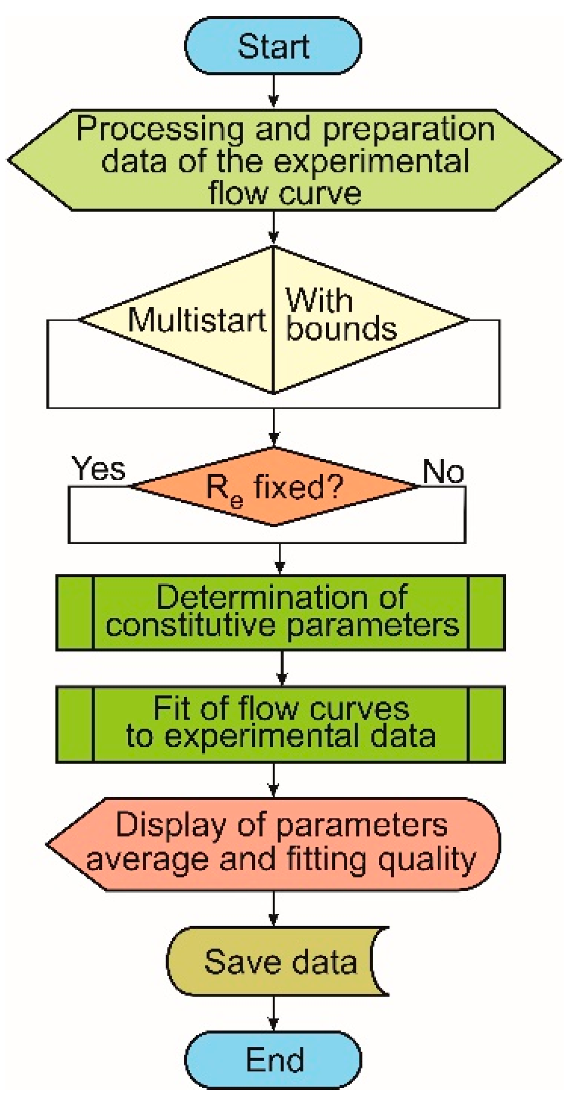
The material constants of the Johnson–Cook constitutive equation were established here using two algorithms. In the first algorithm the constants were established simultaneously by adjusting the flow curves obtained by standardized tensile/compression tests. In the second algorithm the parameters A, B, n were determined separately with the flow curves obtained, before the parameters m and C were identified.
According to the first algorithms, all five constants of the Johnson–Cook constitutive equation were established simultaneously from experimental data of standardized or common tensile/compression tests (see e.g., [
11]) by approximating or adjusting the flow curve obtained in the tests. This task is mathematically no single tasking and depends on the assumed initial values of constitutive parameters. Thus various sets of the constants to be established were obtained for their different initial values. This suggested that the adjustment function of the flow curve is a function with several extreme values. In this case the task of establishing a single set of the constants, which corresponds to the global or greatest extreme value of the adjustment function, could be postulated as:
where
P is the possible amount of parameter sets which consist of the constants
A,
B,
n,
C and
m and are defined in a k-dimensional space
;
S is the amount of parameter sets corresponding to the extreme values of the adjustment function f(X);
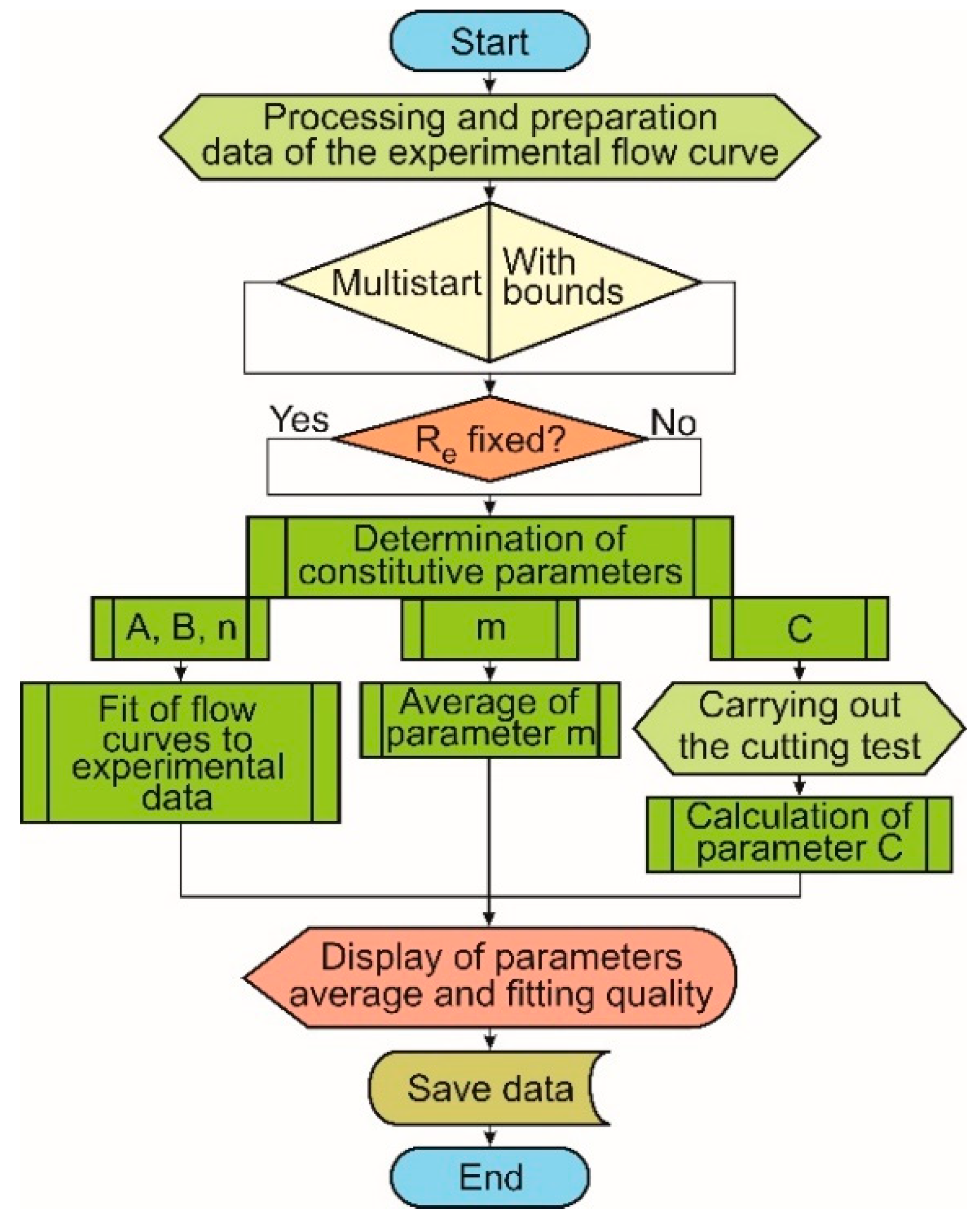
G is the parameter set corresponding to the global extreme value of the adjustment function. The second algorithm is based on the approach that has been developed in the last years. In this approach, the individual terms of the Johnson–Cook constitutive equation and the corresponding physical processes are taken into account separately [
25,
32]. Regarding the classic Johnson–Cook equation, this examination could be expressed as:
where
Kε is the term for strain hardening,
is the term for strain rate sensitivity and
KT is the term for thermal softening. Such a procedure can also be used for establishing the constants of newly developed material models based on the Johnson–Cook constitutive equation [
19,
21,
22,
23,
25,
26].
In the first step of the second algorithm, the constants A, B and n, characterizing the term for strain hardening in the Johnson–Cook constitutive equation, were determined by adjusting the flow curves obtained in standardized tensile/compression tests. Thus, the adjusted coefficient of hardening Kε was established.
In the second step of this algorithm, the thermal softening power coefficient m was established. The constants
A,
B and
n of the strain hardening term, which were established by adjusting the flow curves obtained in tensile/compression tests at varying temperatures, were put in for that purpose. Then the coefficients of correction were established for every temperature used in these tests by means of the following equation [
32]:
An average coefficient of correction
KT was calculated for every tensile/compression test at the respective temperature. Then the coefficient m was established by approximating (adjusting) the calculated range of average correction coefficients with the following equation [
32]:
The constant
C of the strain rate sensitivity term
was determined by means of Oxley’s machining theory [
33] and the extension of Oxley’s machining theory [
16,
34,
35,
36,
37], using kinetic data obtained by orthogonal cutting experiments:
Hence, it was possible to establish the constant
C at the same strain rate as well as under the same conditions of the work material’s hardening and softening like in a real cutting process. The equivalent shear strain
εAB and the equivalent strain rate
in the shear zone AB or primary shear zone were determined according to Oxley [
33]:
where
Φ is the shear angle,
γ is the tool orthogonal rake angle of the tool wedge,
C0 is the thickness ratio of the primary shear zone,
lAB is the length of the shear plane,
VC is the chip speed and
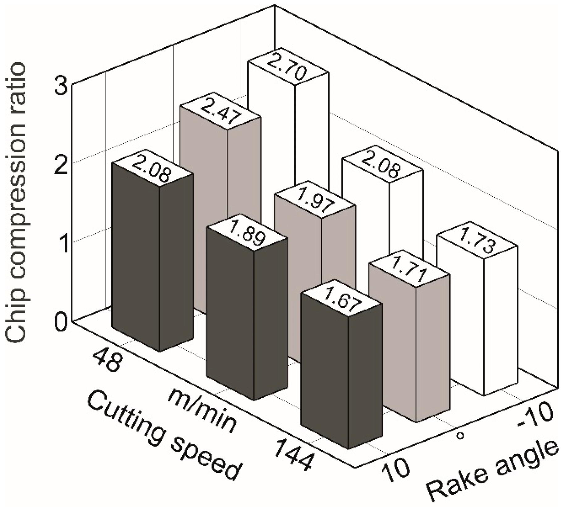
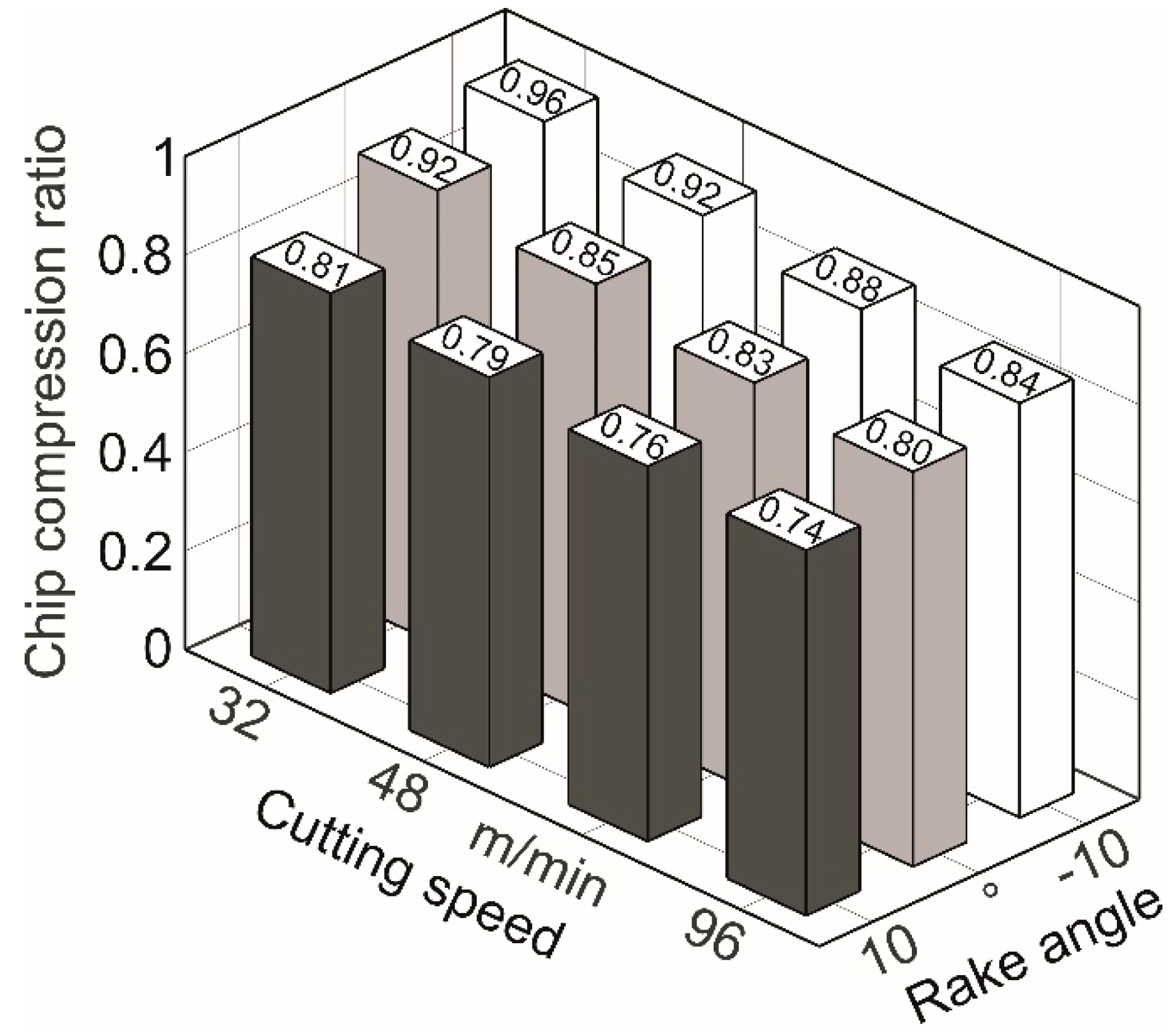
V is the cutting speed. When the chip compression ratio
Ka or the chip thickness
ac is determined by experiment, then the strain
εAB can be established with the following equation [
38,
39]:
The yield point
σs was equated with the shear stress
τAB in the primary shear zone along the conditional shear plane
AB [
16,
35,
36]:
where
FAB is the shear force along the shear plane
AB,
a and
w are the undeformed chip thickness (cutting depth) and the cutting width, respectively. The shear force
FAB was calculated based on the measured cutting force
FX and thrust force
FZ [
16,
40,
41]:
The shear angle
Φ was determined either by experiment due to the measured chip thicknesses a
C (see Equation (12)) [
16] and the chip compression ratio
Ka [
41] (see Equation (13)) or analytically [
40]:
The temperature
TAB which arises due to the plastic deformation in the primary shear zone and is used for establishing the coefficients of correction
KT can be determined with the following equation [
16,
33,
36,
42]:
where
T0 is the room temperature,
η is the parameter to scale the average temperature rise at
AB (
),
β is the proportion of heat conducted into the workpiece,
ρ is the density,
S is the specific heat,
RT is the non-dimensional thermal number, λ is the thermal conductivity of the work material. This task was solved with the algorithms developed for that purpose, as described in
Section 6.
7. Simulation Results
The constitutive parameters calculated using the second (separately) algorithm (see
Section 6) were verified with the simulation of an orthogonal cutting process. For that purpose, a 3D cutting model in the FEM software environment DEFORM 2D/3D™ v. 11.0 (SFTC, Columbus, OH, USA) was worked out for simulating the machining of AISI 1045 steel and Ti-1023 titanium alloy.
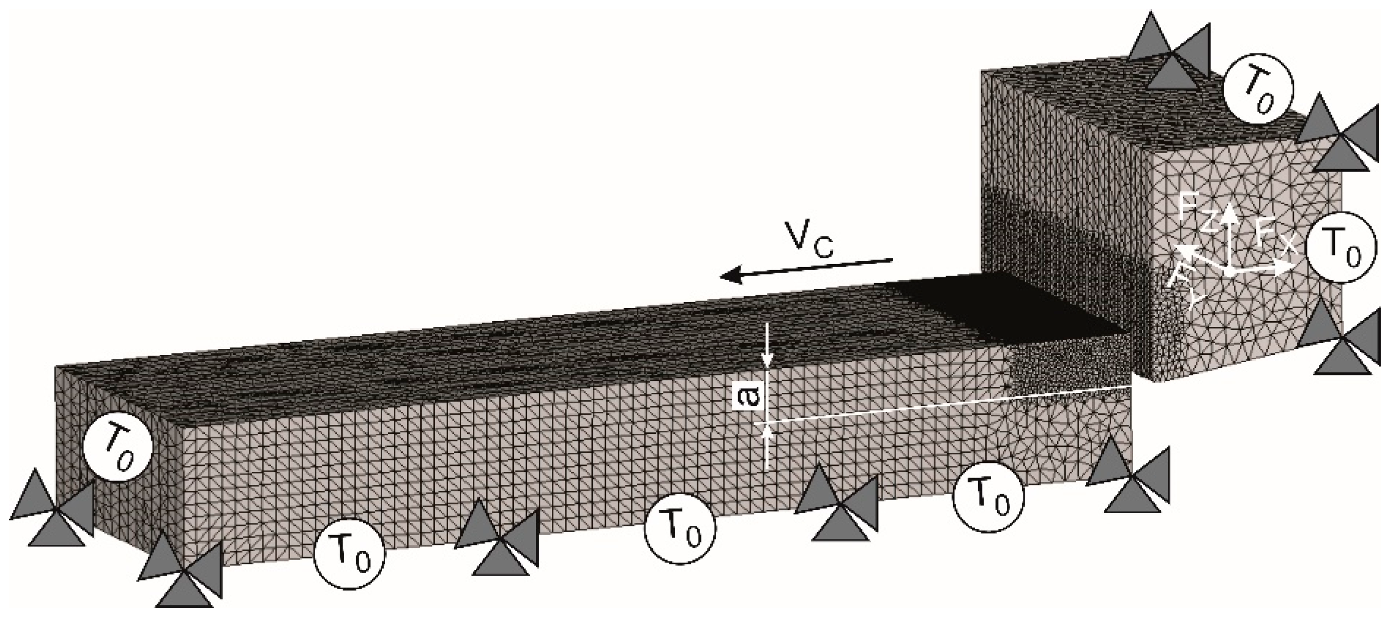
Figure 9 presents the meshed geometrical model.
To improve the efficiency and the precision of the cutting model, the workpiece was meshed more finely in the shear zones as well as in the chip and the tool was also meshed more finely in the contact areas with the workpiece and the chip. The mesh in the remaining areas was established more roughly. The boundary conditions were determined by fixing the workpiece and the tool as well as by the input of the thermal conditions at the boundaries of the respective objects. The bottom of the workpiece was rigidly fixed in the X-, Y- and Z-directions. The rigid fixation of the tool at the back of its rake face in Z-direction prevents its meshing in this direction. The thermal initial conditions at room temperature (RT) were given at the bottom and the left-hand side of the workpiece as well as at the left-hand side and the top of the tool. The working motion of the tool at a cutting speed VC for guaranteeing the cutting process was given by the absolute motion in the negative X-direction.
In order to reproduce the cutting process of the titanium alloy, the Cocroft and Latham model [
4] was used as fracture model and the critical breaking stress was set to 240 MPa. Using a DOE (design of experiments) analysis, it was determined that the breaking stress and the load-carrying capacity of the finite elements were 10% after the fracture. The friction during the contact between the tool and the workpiece was modelled with a hybrid friction model. The model represented a combination of the Coulomb and the shear friction models. Regarding the modelling of the cutting process of AISI 1045 steel, the Coulomb friction coefficient was 0.15 and the plastic friction coefficient of the shear friction model was 0.6. These values were 0.2 and 0.8, respectively, when modelling the cutting process of Ti-1023 titanium alloy.
The functioning of the FEM cutting model was verified by simulating the chip formation, the development of the strain rate in the shear zones as well as the temperature flows in the workpiece during the machining of AISI 1045 steel and Ti-1023 titanium alloy. As an example,
Table 3 presents the cutting characteristics for different process parameters. The analysis of the simulation results indicated that the FEM cutting model was suitable for the further modelling.
The elaborated FEM cutting model and the quality of the developed algorithm for establishing constitutive parameters were verified by means of comparing the resultant forces determined by experiment as well as the cutting temperatures calculated analytically with the corresponding simulated process characteristics.
Table 4 presents the cutting parameters and the tool orthogonal rake angles used in the experimental tests of the machining process for verifying the FEM cutting model.
Table 5 shows the results of the comparison between the simulated and the calculated as well as experimental values of the cutting temperature, the resultant forces and the strain in the chip forming area. The comparison (s. the values of deviation) showed a good agreement and confirmed the validity of the elaborated algorithm as well as the FEM cutting model.
The comparison of the two developed algorithms (see
Section 6) was based on the comparison of the simulated and experimental cutting forces.
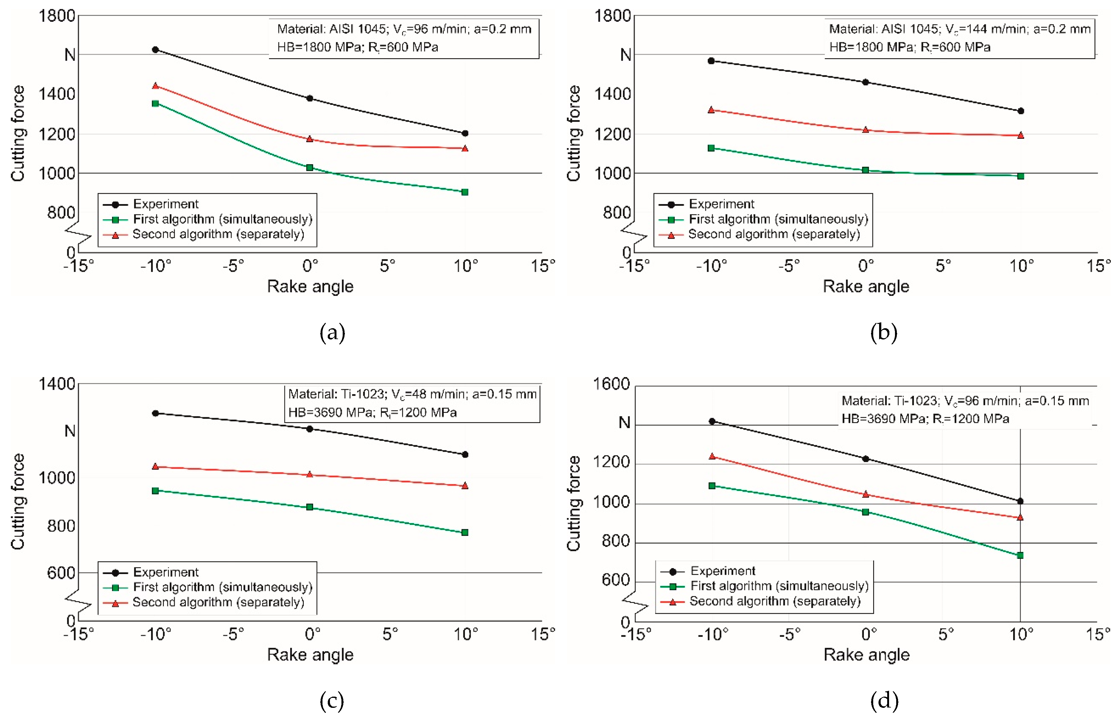
Figure 10 presented this comparison. The
Figure 10a,b show the experimental and simulative data when cutting steel AISI 1045 at 96 m/min and 144 m/min, the
Figure 10c,d show the results of cutting titanium alloy Ti-1023 at the cutting speeds of 48 m/min and 96 m/min, respectively. The deviation between experimental and simulatively defined cutting forces with the constitutive parameters determined by the first (simultaneous) algorithm is in the range of 17% to 30% for machining the steel AISI 1045 and in the range of 22% to 30% for machining the titanium alloy Ti-1023. This deviation in the constitutive parameters determined used the second (separately) algorithm is in the range of 8% to about 17% for the machining of the AISI 1045 steel and in the range of 8% to 18% in the machining of the titanium alloy Ti-1023 (s.
Figure 10 and
Table 5).
The much larger deviation in the experimentally and simulatively determined cutting forces using the first (simultaneous) algorithm is in all likelihood that the first algorithm only ensured the numerical conditions of the fitting. The algorithm does not account for the real physical processes involved in machining such as softening of the material being processed due to thermal action, and additional material hardening due to the increase in strain rate with increasing cutting speed. The physical processes are taken into account in determining the constitutive parameters using the second algorithm, since the different parameters such as m and C are defined under the same conditions as in a real cutting process. As a result, the second algorithm provided significantly better agreement between the experimental and simulatively determined cutting forces.
Author Contributions
Conceptualization, M.S.; Methodology, M.S.; Software, M.S. and P.R.; Validation, M.S.; Formal analysis, M.S. and P.R.; Investigation, M.S. and P.R.; Resources, M.S. and P.R.; Data curation, M.S. and P.R.; Writing—original draft preparation, M.S.; Writing—review and editing, M.S., H.-C.M. and T.S.; Visualization, M.S.; Supervision, H.-C.M. and T.S.; Project administration, H.-C.M. and T.S.; Funding acquisition, H.-C.M. and T.S.
Funding
This study was funded by the German Research Foundation (DFG) in the project HE-1656/153-1 “Development of a Concept for Determining the Mechanical Properties of the Cutting Material in Machining”.
Acknowledgments
The authors would like to thank the German Research Foundation (DFG) for their support, which is highly appreciated.
Conflicts of Interest
The authors declare no conflict of interest.
References
- Mourtzis, D.; Doukas, M.; Bernidaki, D. Simulation in Manufacturing: Review and Challenges. Procedia CIRP 2014, 25, 213–229. [Google Scholar] [CrossRef]
- Arrazola, P.J.; Özel, T.; Umbrello, D.; Davies, M.; Jawahir, I. Recent advances in modelling of metal machining processes. CIRP Ann. Manuf. Technol. 2013, 62, 695–718. [Google Scholar] [CrossRef]
- Özel, T.; Sima, M.; Srivastava, A. Finite Element Simulation of High Speed Machining Ti-6Al-4V Alloy using Modified Material Models. Trans. NAMRI/SME 2010, 38, 49–56. [Google Scholar]
- Storchak, M.; Jiang, L.; Xu, Y.; Li, X. FEM Modelling for the Cutting Process of the Titanium Alloy Ti10V2Fe3Al. Prod. Eng. Res. Dev. 2016, 10, 509–517. [Google Scholar] [CrossRef]
- Arrazola, P.J.; Kortabarria, A.; Madariaga, A.; Esnaola, J.A.; Fernandez, E.; Cappelini, C.; Ulutan, D.; Özel, T. On the machining induced residual stresses in IN718 nickel-based alloy: Experiments and predictions with finite element simulation. Simul. Modell. Pract. Theory 2014, 41, 87–103. [Google Scholar] [CrossRef]
- Kushner, V.; Storchak, M. Modelling the material resistance to cutting. Int. J. Mech. Sci. 2017, 126, 44–54. [Google Scholar] [CrossRef]
- Heisel, U.; Kryvoruchko, D.V.; Zaloha, V.A.; Storchak, M.; Stehle, T. Thermomechanische Materialmodelle zur Modellierung von Zerspanprozessen. ZWF 2009, 6, 482–491. [Google Scholar] [CrossRef]
- Johnson, G.R.; Cook, W.H. A constitutive model and data for metals subjected to large strains, high strain and high temperatures. In Proceedings of the 7th International Symposium on Ballistics, The Hague, The Netherlands, 19–21 April 1983; pp. 541–547. [Google Scholar]
- El-Magd, E.; Treppman, C.; Korthäuer, M. Constitutive Modelling of CK45N, AlZnMgCu1.5 and Ti-6Al-4V in a wide range of Strain Rate and Temperature. J. Phys. IV France 2003, 110, 141–146. [Google Scholar]
- Nieslony, P.; Grzesik, W. Sensitivity Analysis of the Constitutive Models in FEM-Based Simulation of the Cutting Process. J. Mach. Eng. 2013, 13, 106–116. [Google Scholar]
- Zabel, A.; Rödder, T.; Tiffe, M. Material testing and chip formation simulation for different heat treated workpieces of 51CrV4 steel. Procedia CIRP 2017, 58, 181–186. [Google Scholar] [CrossRef]
- Burley, M.; Campbell, J.E.; Dean, J.; Clyne, T.W. Johnson–Cook parameter evaluation from ballistic impact data via iterative FEM modelling. Int. J. Impact Eng. 2018, 112, 180–192. [Google Scholar] [CrossRef]
- Chandrasekaran, H.; Saoubi, R.M.; Chazal, H. Modeling of Material Flow Stress in Chip Formation Process from Orthogonal Milling and Split Hopkinson Bar Test. Int. J. Mach. Sci. Technol. 2005, 9, 131–145. [Google Scholar] [CrossRef]
- Kreyszig, E. Advanced Engineering Mathematics, 10th ed.; John Wiley & Sons Ltd.: New York, NY, USA, 2011; 1283p. [Google Scholar]
- Özel, T.; Altan, T. Determination of workpiece stress and friction at the chip-tool contact for high speed cutting. Int. J. Mach. Tools Manuf. 2000, 40, 133–152. [Google Scholar] [CrossRef]
- Özel, T.; Zeren, E. A Methodology to Determine Work Material Flow Stress and Tool-Chip Interfacial Friction Properties by Using Analysis of Machining. ASME J. Manuf. Sci. Eng. 2006, 128, 119–129. [Google Scholar] [CrossRef]
- Denkena, B.; Grove, T.; Dittrich, M.A.; Niederwestberg, D.; Lahres, M. Inverse Determination of Constitutive Equations and Cutting Force Modelling for Complex Tools Using Oxley’s Predictive Machining Theory. Procedia CIRP 2015, 31, 405–410. [Google Scholar] [CrossRef]
- Bäker, M. A new method to determine material parameters from machining simulations using inverse identification. Procedia CIRP 2015, 31, 399–404. [Google Scholar] [CrossRef]
- Klocke, F.; Lung, D.; Buchkremer, S. Inverse Identification of the Constitutive Equation of Inconel 718 and AISI 1045 from FE Machining Simulations. Procedia CIRP 2013, 8, 212–217. [Google Scholar] [CrossRef]
- Özel, T.; Karpat, Y. Identification of constitutive material model parameters for high-strain rate metal cutting conditions using evolutionary computational algorithms. Mater. Manuf. Process 2007, 22, 659–667. [Google Scholar] [CrossRef]
- Eisseler, R.; Drewle, K.; Grötzinger, K.; Möhring, H.-C. Using an inverse cutting simulation-based method to determine the Johnson–Cook material constants of heat-treated steel. Procedia CIRP 2018, 77, 26–29. [Google Scholar] [CrossRef]
- Nemat-Nasser, S.; Guo, W.-G.; Nesterenko, V.; Indrakanti, S.S.; Gu, Y.-B. Dynamic response of conventional and hot isostatically pressed Ti6Al4V alloys: Experiments and modeling. Mech. Mater. 2001, 33, 425–439. [Google Scholar] [CrossRef]
- Calamaz, M.; Coupard, D.; Girot, F. A new material model for 2D numerical simulation of serrated chip formation when machining titanium alloy Ti–6Al–4V. Int. J. Mach. Tools Manuf. 2008, 48, 275–288. [Google Scholar] [CrossRef]
- Ducobu, F.; Rivière-Lorphèvre, E.; Filippi, E. On the importance of the choice of the parameters of the Johnson–Cook constitutive model and their influence on the results of a Ti6Al4V orthogonal cutting model. Int. J. Mech. Sci. 2017, 122, 143–155. [Google Scholar] [CrossRef]
- Sima, M.; Özel, T. Modified material constitutive models for serrated chip formation simulations and experimental validation in machining of titanium alloy Ti-6Al-4V. Int. J. Mach. Tools Manuf. 2010, 50, 943–960. [Google Scholar] [CrossRef]
- Umbrello, D.; Rizutti, S.; Outeiro, J.C.; Shivpuri, R.; M’Saoubi, R. Hardness-based flow stress for numerical simulation of hard machining AISI H13 tool steel. J. Mater. Process. Technol. 2008, 199, 64–73. [Google Scholar] [CrossRef]
- Denguir, L.; Outeiro, J.C.; Fromentin, G.; Vignal, V.; Besnard, R. Orthogonal cutting simulation of OFHC copper using a new constitutive model considering the state of stress and the microstructure effects. Procedia CIRP 2016, 46, 238–241. [Google Scholar] [CrossRef]
- Santos, T.; Outeiro, J.C.; Rossi, R.; Rosa, P. A new methodology for evaluation of mechanical properties of materials at very high rates of loading. Procedia CIRP 2017, 58, 481–486. [Google Scholar] [CrossRef]
- Laakso, S.; Niemi, E. Modified Johnson–Cook flow stress model with thermal softening damping for finite element modeling of cutting. Proc. IMechE Part B J. Eng. Manuf. 2016, 230, 241–253. [Google Scholar] [CrossRef]
- Chen, G.; Ren, C.; Yu, W.; Yang, X.; Zhang, L. Application of genetic algorithms for optimizing the Johnson–Cook constitutive model parameters when simulating the titanium alloy Ti-6Al-4V machining process. Proc. IMechE Part B J. Eng. Manuf. 2012, 226, 1287–1297. [Google Scholar] [CrossRef]
- Malakizadi, A.; Cedergren, S.; Sadik, I.; Nyborg, L. Inverse identification of flow stress in metal cutting process using Response Surface Methodology. Simul. Modell. Pract. Theory 2016, 60, 40–53. [Google Scholar] [CrossRef]
- Krivoruchko, D.V.; Zaloga, V.A. Cutting Processes Modeling with Finite Elements Method; University Book: Sumi, Ukraine, 2012; 496 p. (In Russian) [Google Scholar]
- Oxley, P.L.B. Mechanics of Machining. An Analytical Approach to Assessing Machinability; Ellis Horwood: Chichester, UK, 1989; 242 p. [Google Scholar]
- Adibi-Sedeh, A.H.; Madhavan, V.; Bahr, B. Extension of Oxley’s Analysis of Machining to Use Different Material Models. J. Manuf. Sci. Eng. 2003, 125, 656–666. [Google Scholar] [CrossRef]
- Lalwani, D.I.; Mehta, N.K.; Jain, P.K. Extension of Oxley’s predictive machining theory for Johnson-and Cook flow stress model. J. Mater. Process. Technol. 2009, 209, 5305–5312. [Google Scholar] [CrossRef]
- Chen, Y.; Li, H.; Wang, J. Further Development of Oxley’s Predictive Force Model for Orthogonal Cutting. Mach. Sci. Technol. 2015, 19, 86–111. [Google Scholar] [CrossRef]
- Xiong, L.; Wang, J.; Gan, Y.; Li, B.; Fang, N. Improvement of algorithm and prediction precision of an extended Oxley’s theoretical model. Int. J. Adv. Manuf. Technol. 2015, 77, 1–13. [Google Scholar] [CrossRef]
- Zorev, N.N. Metal Cutting Mechanics; Pergamon Press GmbH: Frankfurt am Main, Germany, 1966; 526p. [Google Scholar]
- Kushner, V.; Storchak, M. Determining mechanical characteristics of material resistance to deformation in machining. Prod. Eng. Res. Dev. 2014, 8, 679–688. [Google Scholar] [CrossRef]
- Tsekhanov, J.; Storchak, M. Development of analytical model for orthogonal cutting. Prod. Eng. Res. Dev. 2015, 9, 247–255. [Google Scholar] [CrossRef]
- Heisel, U.; Kushner, V.; Storchak, M. Effect of machining conditions on specific tangential forces. Prod. Eng. Res. Dev. 2012, 6, 621–629. [Google Scholar] [CrossRef]
- Möhring, H.-C.; Kushner, V.; Storchak, M.; Stehle, T. Temperature calculation in cutting zones. CIRP Ann. Manuf. Technol. 2018, 67, 61–64. [Google Scholar] [CrossRef]
- Material Property Data. Available online: http://www.matweb.com (accessed on 19 April 2019).
- Ugray, Z.; Lasdon, L.S.; Plummer, J.C.; Glover, F.; Kelly, J.P.; Marti, R. Scatter Search and Local NLP Solvers: A Multistart Framework for Global Optimization. INFORMS J. Comput. 2007, 19, 328–340. [Google Scholar] [CrossRef]
© 2019 by the authors. Licensee MDPI, Basel, Switzerland. This article is an open access article distributed under the terms and conditions of the Creative Commons Attribution (CC BY) license (http://creativecommons.org/licenses/by/4.0/).


