Mold-Level Prediction for Continuous Casting Using VMD–SVR


Abstract
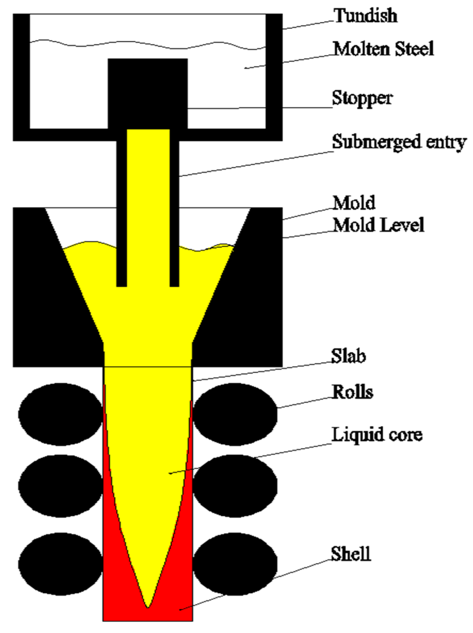
:1. Introduction
2. Basic Algorithm Research
2.1. Variational Mode Decomposition
- Step 1:
- Initialize , , λ1 and n to zero;
- Step 2:
- n = n + 1, execute the entire loop;
- Step 3:
- Execute the loop k = k + 1 until k = K, update uk: ;
- Step 4:
- Execute the loop k = k + 1, until k = K, update ωk: ;
- Step 5:
- Use to update λ;
- Step 6:
- Given the discrimination condition ε > 0, if the iteration stop condition is satisfied, all the cycles are stopped and the result is output, and K IMFs are obtained.
2.2. Support Vector Machine
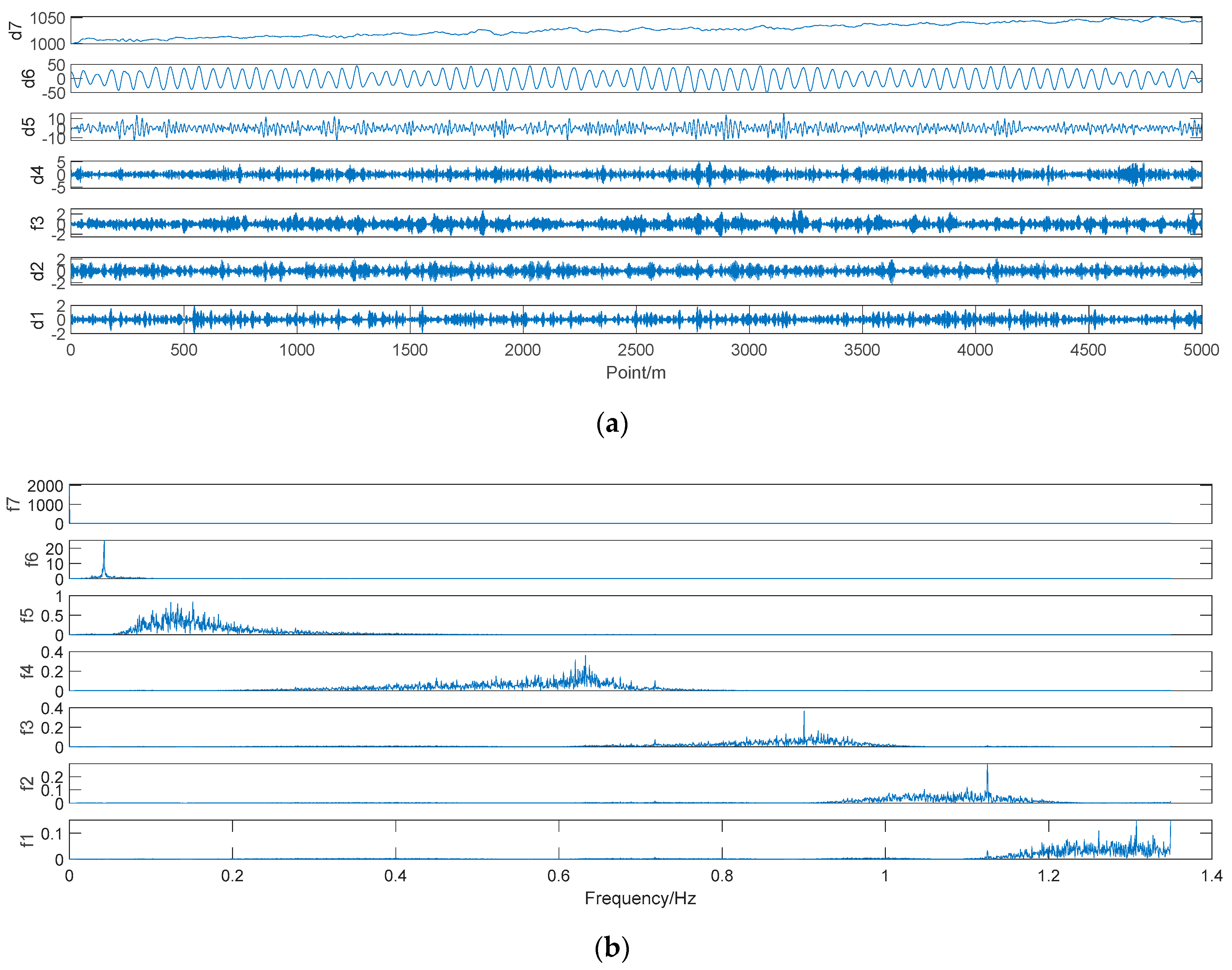
2.3. Empirical Mode Decomposition
- (1)
- In the entire data set, the number of extreme values and the number of zero crossings must be equal or at most have one point of difference.
- (2)
- At any point, the average defined by the local maximum envelope and the minimum envelope is zero.
2.4. Wavelet Threshold Denoising
- (1)
- The noisy signal is transformed by wavelet transform. A wavelet basis is selected to determine the level N of the wavelet decomposition at the same time, and then the signal x is decomposed by the N-level wavelet.
- (2)
- The wavelet coefficients are thresholder. In order to keep the overall shape of the signal unchanged and keep the effective signal, the hard threshold, soft threshold or other threshold methods are used to quantify the sparseness of each layer after decomposition.
- (3)
- The inverse wavelet transform is performed, and the signal is reconstructed.
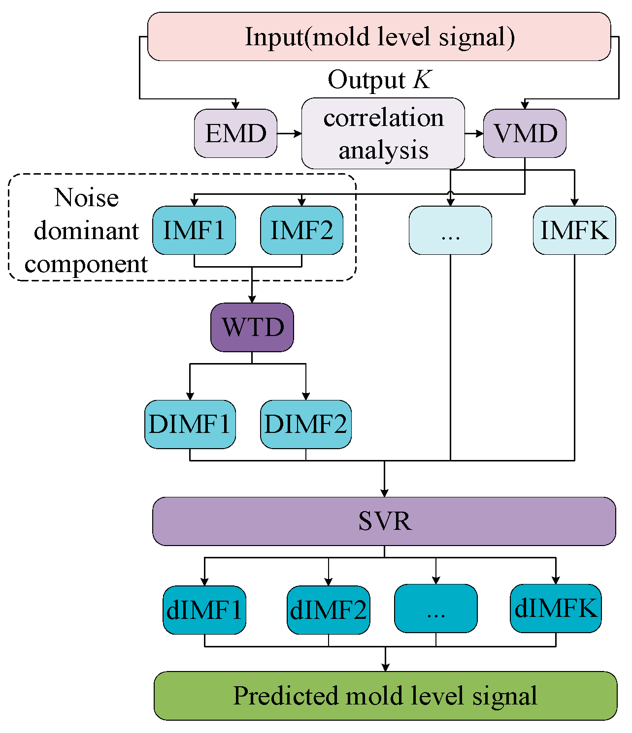
3. Hybrid Algorithm Research
- Step 1:
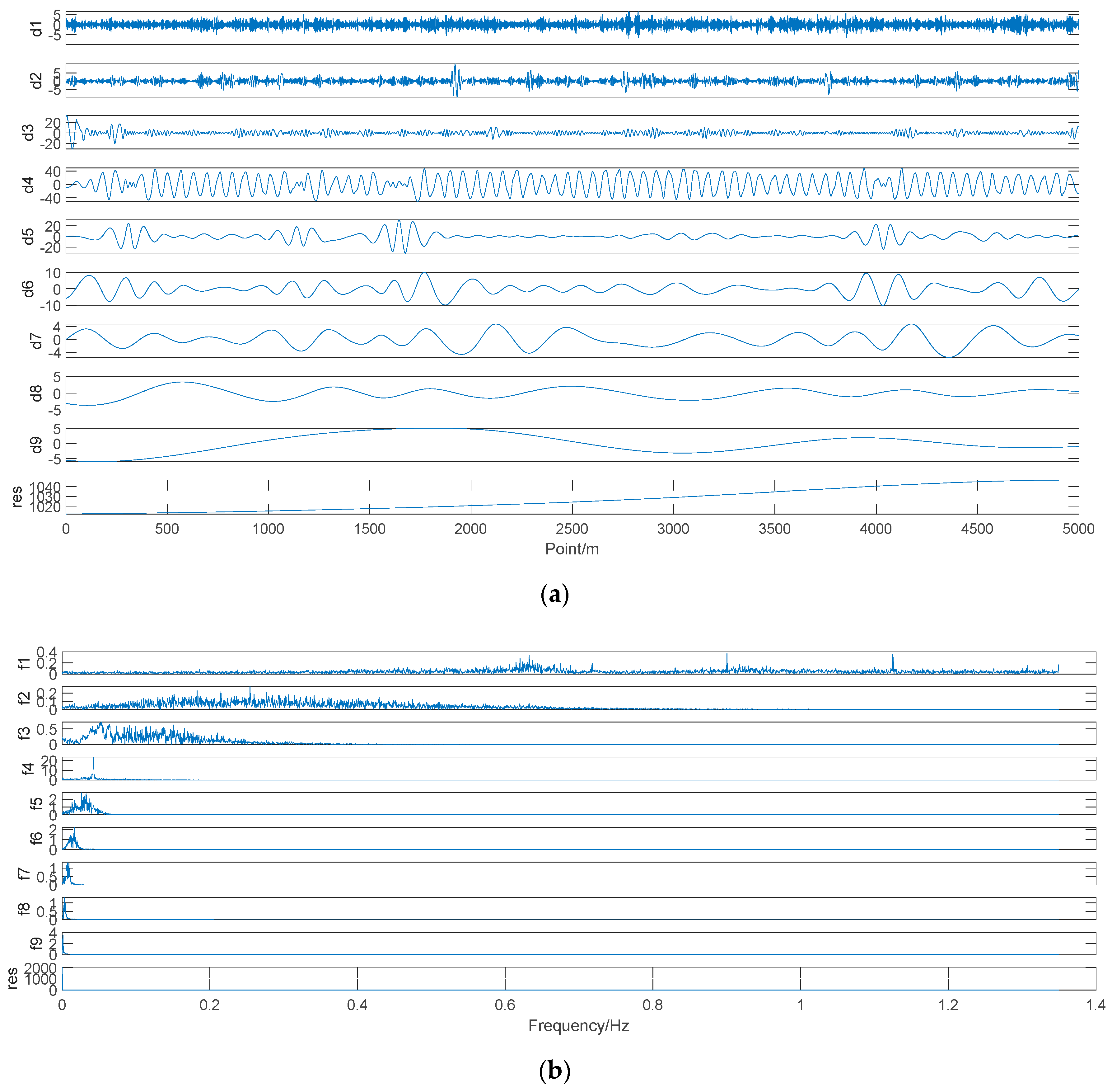
- Adaptively decompose the mold-level data based on the EMD algorithm to obtain several IMFs;
- Step 2:
- The K value of the key parameter of the VMD is obtained by the correlation analysis between the IMFs;
- Step 3:
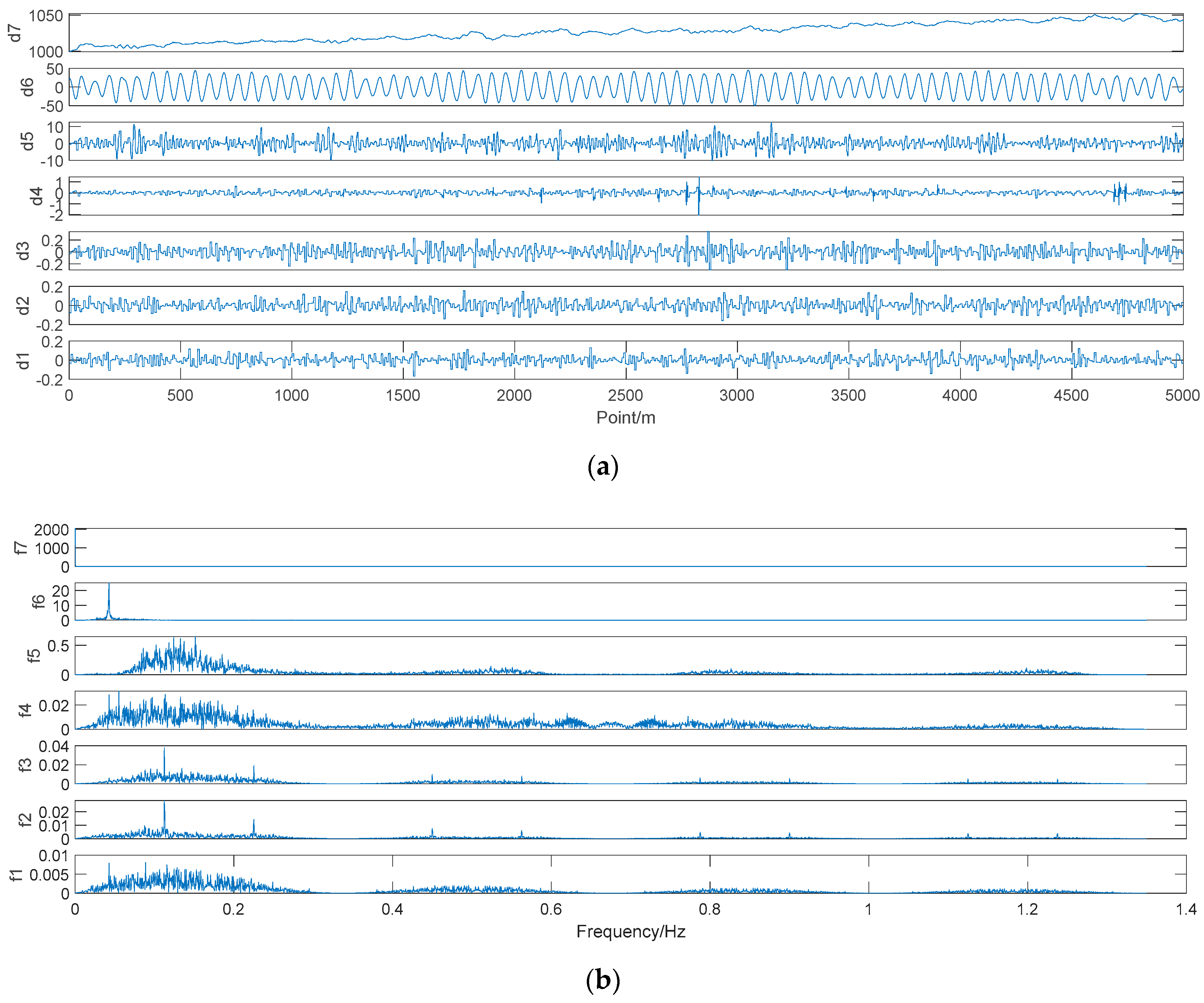
- Perform VMD decomposition on the original signal based on K to obtain K IMFs;
- Step 4:
- Denoise the noise related component;
- Step 5:
- Perform SVR on the denoised IMFs and other IMFs to obtain the predicted IMFs;
- Step 6:
- Reconstruct the predicted component and obtain the predicted signal.
4. Experimental Studies
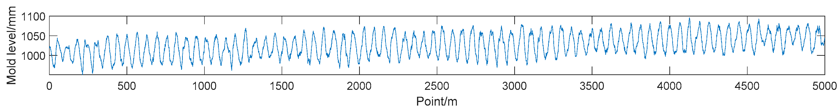
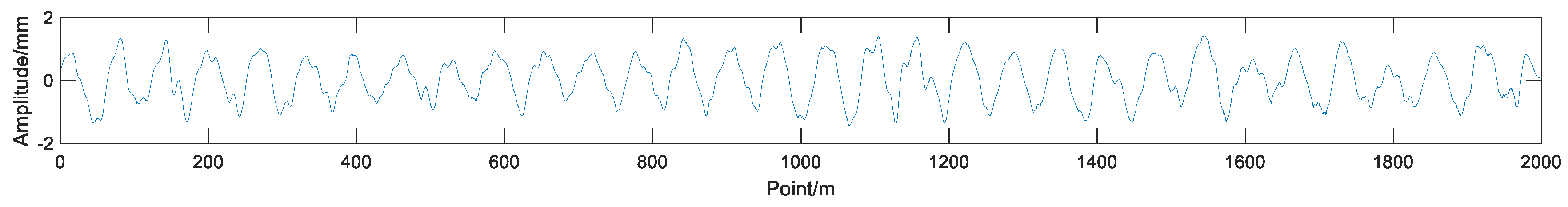
4.1. Problem Prescription
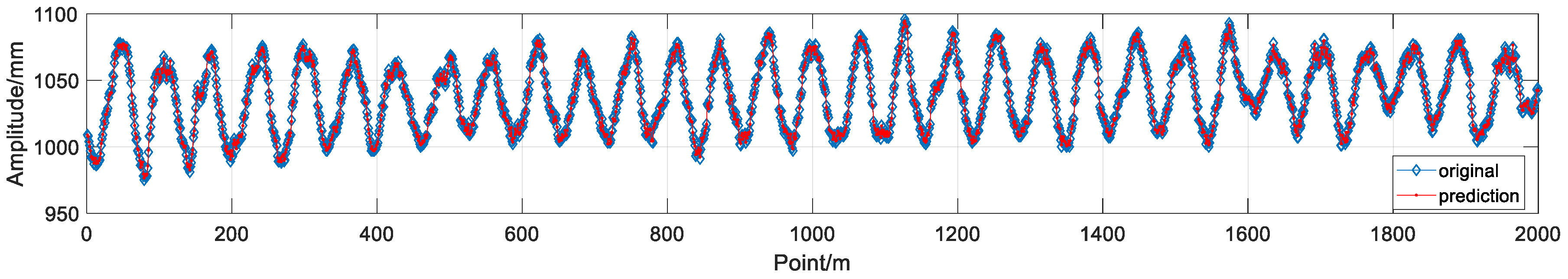
4.2. Mold-Level Prediction Based on VMD–SVR Model
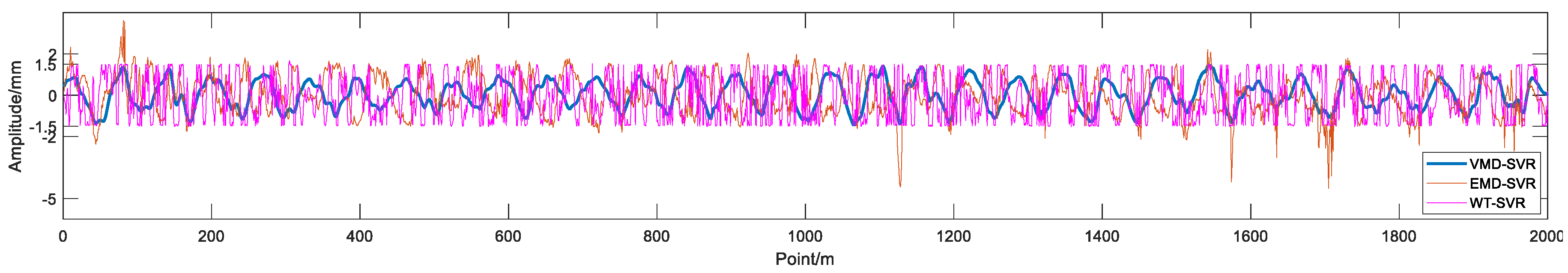
5. Prediction Results and Analysis
6. Conclusions
- (1)
- The VMD–SVR algorithm can be used to establish the prediction model, removing noise while retaining the effective information in the data, with good denoising performance and sampling rate robustness;
- (2)
- In comparison with the results of the other two algorithms, the three indicators of the VMD–SVR algorithm are significantly better than those of the other two algorithms. The RMSE index is improved by 36.1%, the MAPE index are improved by 37.5%, the R is improved by 3%, and the MAE index is improved by 37.6%;
- (3)
- The use of mold-level prediction methods in the research on mold prediction control represents a future research direction. Accurate mold-level prediction provides a new idea for mold-level prediction control, which has important practical significance;
- (4)
- Using the accurately predicted mold-level data for mold-level control, the sliding nozzle and roller pressure disturbances can be well restrained. The anti-interference ability of the mold level control system is enhanced.
Author Contributions
Funding
Acknowledgments
Conflicts of Interest
References
- Ataka, M. Rolling technology and theory for the last 100 years: The contribution of theory to innovation in strip rolling technology. ISIJ Int. 2015, 55, 89–102. [Google Scholar] [CrossRef]
- Jin, X.; Chen, D.F.; Zhang, D.J.; Xie, X. Water model study on fluid flow in slab continuous casting mould with solidified shell. Ironmak. Steelmak. 2011, 38, 155–159. [Google Scholar] [CrossRef]
- Guo, G.; Wang, W.; Chai, T. Predictive mould level control in a continuous casting line. Control Theory Appl. 2011, 18, 714–717. [Google Scholar]
- Tong, C.; Xiao, L.; Peng, K.; Li, J. Constrained generalized predictive control of mould level based on genetic algorithm. Control Decis. 2009, 24, 1735–1739. [Google Scholar]
- Qiao, G.; Tong, C.; Sun, Y. Study on Mould level and casting speed coordination control based on ADRC with DRNN optimization. Acta Autom. Sin. 2007, 33, 641–648. [Google Scholar]
- Huang, N.E.; Shen, Z.; Long, S.R.; Wu, M.C.; Shih, H.H.; Zheng, Q.; Yen, N.; Tung, C.C.; Liu, H.H. The empirical mode decomposition and the Hilbert spectrum for nonlinear and non-stationary time series analysis. Proc. R. Soc. A-Math. Phys. 1998, 454, 903–995. [Google Scholar] [CrossRef]
- Konstantin, D.; Dominique, Z. Variational mode decomposition. IEEE Trans. Signal Process. 2014, 62, 531–544. [Google Scholar]
- Lee, W.J.; Hong, J. A hybrid dynamic and fuzzy time series model for mid-term power load predicting. Int. J. Electr. Power Energy Syst. 2015, 64, 1057–1062. [Google Scholar] [CrossRef]
- Dai, S.; Niu, D.; Li, Y. Daily peak load predicting based on complete ensemble empirical mode decomposition with adaptive noise and support vector machine optimized by modified grey wolf optimization algorithm. Energies 2018, 11, 163. [Google Scholar] [CrossRef]
- Lynch, P. The origins of computer weather prediction and climate modeling. J. Comput. Phys. 2008, 227, 3431–3444. [Google Scholar] [CrossRef]
- Gaudioso, M.; Gorgone, E.; Labbe, M.; Rodríguez-Chía, A.M. Lagrangian relaxation for SVM feature selection. Comput. Oper. Res. 2017, 87, 137–145. [Google Scholar] [CrossRef] [Green Version]
- Wang, J.; Shi, P.; Jiang, P.; Hu, J.; Qu, S.; Chen, X.; Chen, Y.; Dai, Y.; Xiao, Z. Application of BP neural network algorithm in traditional hydrological model for flood predicting. Water 2017, 9, 48. [Google Scholar] [CrossRef]
- He, F.; Zhang, L. Mold breakout prediction in slab continuous casting based on combined method of GA-BP neural network and logic rules. Int. J. Adv. Manuf. Technol. 2018, 95, 4081–4089. [Google Scholar] [CrossRef]
- Fan, G.F.; Peng, L.L.; Hong, W.C.; Sun, F. Electric load predicting by the SVR model with differential empirical mode decomposition and auto regression. Neurocomputing 2016, 173, 958–970. [Google Scholar] [CrossRef]
- Nie, H.; Liu, G.; Liu, X.; Wang, Y. Hybrid of ARIMA and SVMs for short-term load predicting, 2012 international conference on future energy, environment, and materials. Energy Procedia 2012, 16, 1455–1460. [Google Scholar] [CrossRef]
- Liu, Y.; Gao, Z. Enhanced just-in-time modelling for online quality prediction in BF ironmaking. Ironmak. Steelmak. 2015, 42, 321–330. [Google Scholar] [CrossRef]
- Shen, B.Z.; Shen, H.F.; Liu, B.C. Water modelling of level fluctuation in thin slab continuous casting mould. Ironmak. Steelmak. 2009, 36, 33–38. [Google Scholar] [CrossRef]
- Hong, W.-C. Chaotic particle swarm optimization algorithm in a support vector regression electric load predicting model. Energy Convers. Manag. 2009, 50, 105–117. [Google Scholar] [CrossRef]
- Ghosh, S.K.; Ganguly, S.; Chattopadhyay, P.P.; Datta, S. Effect of copper and microalloying (Ti, B) addition on tensile properties of HSLA steels predicted by ANN technique. Ironmak. Steelmak. 2009, 36, 125–132. [Google Scholar] [CrossRef]
- Voyant, C.; Muselli, M.; Paoli, C.; Nivet, M.-L. Numerical weather prediction (NWP) and hybrid ARMA/ANN model to predict global radiation. Energy 2012, 39, 341–355. [Google Scholar] [CrossRef] [Green Version]
- Lei, Y.G.; Lin, J.; He, Z.J.; Zuo, M.J. A review on empirical mode decomposition in fault diagnosis of rotating machinery. Mech. Syst. Sig. Process. 2013, 35, 108–126. [Google Scholar] [CrossRef]
- Tomic, M. Wavelet transforms with application in signal denoising. Ann. DAAAM Proc. 2008, 1401–1403. [Google Scholar]
- El B’charri, O.; Latif, R.; Elmansouri, K.; Abenaou, A.; Jenkal, W. ECG signal performance de-noising assessment based on threshold tuning of dual-tree wavelet transform. Biomed. Eng. Online 2017, 16, 26. [Google Scholar] [CrossRef] [PubMed]
- Varady, P. Wavelet-Based Adaptive Denoising of Phonocardiographic Records. In Proceedings of the 23rd Annual International Conference on IEEE-Engineering-in-Medicine-and-Biology-Society, Istanbul, Turkey, 25–28 October 2001; pp. 1846–1849. [Google Scholar]


| Project | Specification |
|---|---|
| Continuous-casting machine model | Curved continuous caster |
| Secondary cooling category | Aerosol cooling, dynamic water distribution |
| Gap control | Remote adjustment, dynamic soft reduction |
| Basic arc radius/mm | 9500 |
| Mold length/mm | 900 |
| Metallurgical length/mm | 39,200 |
| Mold vibration frequency/time/min | 25–400 |
| Mold vibration amplitude/mm | 2–10 |
| Slab width/mm | 900–2150 |
| Slab thickness/mm | 230/250 |
| Working speed/m/min | 0.8–2.03 |
| Actual cast speed/m/min | 1.3 |
| Slab section size/mm × mm | 230 × 1350 |
| Mold oscillation frequency/Hz | 1.36 |
| Actual oscillation amplitude of mold/mm | 60 |
| IMF | Correlation Coefficient |
|---|---|
| IMF 1 | 0.06 |
| IMF 2 | 0.0906 |
| IMF 3 | 0.1348 |
| IMF 4 | 0.8474 |
| IMF 5 | 0.1579 |
| IMF 6 | 0.0196 |
| IMF 7 | 0.0061 |
| IMF 8 | 0.0598 |
| IMF 9 | 0.0585 |
| IMF | Correlation Coefficient |
|---|---|
| IMF 1 | 0.0279 |
| IMF 2 | 0.0360 |
| IMF 3 | 0.0429 |
| IMF 4 | 0.0638 |
| IMF 5 | 0.1769 |
| IMF 6 | 0.8847 |
| IMF 7 | 0.4560 |
| Algorithm | R | RMSE | MAE | MAPE |
|---|---|---|---|---|
| WT–SVR | 0.9733 | 1.0824 | 0.9601 | 0.092316 |
| EMD–SVR | 0.9691 | 0.9480 | 0.7662 | 0.073558 |
| VMD–SVR | 0.9992 | 0.6910 | 0.5983 | 0.057686 |
© 2019 by the authors. Licensee MDPI, Basel, Switzerland. This article is an open access article distributed under the terms and conditions of the Creative Commons Attribution (CC BY) license (http://creativecommons.org/licenses/by/4.0/).
Share and Cite
Su, W.; Lei, Z.; Yang, L.; Hu, Q. Mold-Level Prediction for Continuous Casting Using VMD–SVR. Metals 2019, 9, 458. https://doi.org/10.3390/met9040458
Su W, Lei Z, Yang L, Hu Q. Mold-Level Prediction for Continuous Casting Using VMD–SVR. Metals. 2019; 9(4):458. https://doi.org/10.3390/met9040458
Chicago/Turabian StyleSu, Wenbin, Zhufeng Lei, Ladao Yang, and Qiao Hu. 2019. "Mold-Level Prediction for Continuous Casting Using VMD–SVR" Metals 9, no. 4: 458. https://doi.org/10.3390/met9040458