Hot Deformation Process Analysis and Modelling of X153CrMoV12 Steel

Abstract

Analysis of the high temperature plastic behavior of high-strength steel X153CrMoV12 was developed in the temperature range of 800–1200 °C and the deformation rate in the range of 0.001–10 s⁻¹ to the maximum value of the true strain 0.9%. Microstructural changes were observed using light optical microscopy (LOM) as well as atomic force microscopy (AFM). The effect of hot deformation temperature on true stress, peak stress and true strain was evaluated from the respective flow curves. Based on these results, steel transformation was discussed from the dynamic recovery and recrystallization point of view. Furthermore, a present model, taking into account the Zener–Hollomon parameter, was developed to predict the true stress and strain over a wide range of temperatures and strain rates. Using constitutive equations, material parameters and activation energy were derived, which can be subsequently applied to other models related to hot deformation behavior of selected tool steels. The experimental data were compassed to the ones obtained by the predictive model with the correlation coefficient R = 0.98267. These results demonstrate an appropriate applicability of the model for experimental materials in hot deformation applications.

1. Introduction

The present work deals with the use of dilatometry to determine the deformation resistance of ledeburitic steels and points to its dependence on the deformation rate and the deformation temperature. The contributions of Pernis et al. [1] and Garofalo [2] can be considered as a major work in the field of the high temperature deformation. A good description of the nature of plastometry is given in References [3,4]. Furthermore, the effect of deformation parameters on the no-recrystallization temperature in steels is well described in References [5,6]. A classic response under compression at high temperature is shown in Figure 1. This curve consists of two coordinates, the true stress and strain, while the elastic deformation is negligible. Four characteristic points can be observed in the profile of the deformation curve, whereby the point [0, σ₀] represents the onset of the plastic deformation. In this context, the stress σ₀ can be considered as the compression stress limit. The subsequent point, characterized by coordinates [ε_p, σ_p], represents the maximum stress value of the stress–strain curve and it is designated as the peak stress [7,8].

Analogously, the deformation value, where the deformation curve reaches the maximum, is referred as the peak deformation ε_p. Furthermore, the point coordinates [ε_i, σ_i] define the inflection point of the deformation curve. Finally, at the point [ε_ss, σ_ss] the curve reaches a steady state, at which a dynamic equilibrium occurs between hardening and softening process in a deformed material. Dilatometry makes it possible to perform the pressure tests under defined conditions, in terms of temperature, strain and strain rate in order to acquire high temperature deformation stress–strain curves [9,10,11].

Some currently produced steels with extreme high content of carbide forming elements are widely known as ledeburitic steels [12,13,14,15]. Ledeburitic structure is typical for white cast irons with carbon content above 2.11 wt.% as can be seen in the Fe–Fe₃C metastable binary diagram in Figure 2. However, alloying elements, present in the ledeburitic steel, extend the area of ferrite and narrow the area of austenite. Consequently, eutectoid point S and point of maximum solubility of carbon in austenite—E are moved to the lower carbon contents. Due to this effect, ledeburite is present in structure of these steels at the carbon content below 2.11 wt.% [16]. The common carbon content in ledeburitic steels is higher than 0.7 wt.%. At lower carbon contents, a certain amount of δ–ferrite is usually present in the microstructure, causing an adverse decrease of hardness. Essential alloying elements of ledeburitic steels are Cr, V, W and Mo. All of these elements form carbides and thus noticeably affect deformability, plasticity, hardening and softening mechanisms of the steel during heat treatment. Nb, Al, B and Si could also be used as alloying elements to improve the above-mentioned properties of the ledeburitic steels. In the soft-annealed condition, the contents of carbides are in the range of 20–30 wt.% and in the quenched condition in the range of 10–25 wt.%, depending on the chemical composition [17].

The main purpose of the present work is to investigate the impact of the hot working parameters such as temperature and deformation rate on flow curves and materials parameters of X153CrMoV12 steel. In addition, the influence of these parameters on the microstructural evolution during hot deformation is thoroughly investigated.

2. Materials and Methods

The base material used in the present experiments is a high alloyed tool steel X153CrMoV12 used in the engineering industry. It is a chromium-vanadium steel with the high hardenability suitable for quenching in oil and air [9]. The steel is characterized by the high wear resistance and very high tensile strength (up to 2180 MPa), being mostly used for cutting tools, such as stretching and extruding mandrels, profile blades and complex shaped milling cutters. The chemical composition of experimental samples was verified by a spectral analyzer Q4 TASMAN (Bruker, Karlsruhe, Germany) and it is presented in

Table 1. Chemical composition of the X153CrMoV12 examined steel (wt.%).

ISO 4967	C	Mn	Si	Cr	Mo	V
Min.	1.45	0.20	0.10	11.00	0.70	0.70
Max.	1.60	0.60	0.40	13.00	1.00	1.00
Spectral analysis	1.53	0.40	0.35	12.00	1.00	1.00

. Its basic mechanical and physical properties are listed in

Table 2. Basic mechanical and physical properties of the X153CrMoV12 steel.

Mechanical and Physical Properties	Tensile Strength Rm [MPa]	Young’s Modulus E [GPa]	Thermal Conductivity [W·m−1·°C]	Hardness * [HV]	Specific Heat [J·kg−1·°C]
Value	2180	210	20	790	460

* Oil-quenched.

.

The base material was supplied in the form of bars with a diameter of 10 mm and a length of 1000 mm. The supplied material is produced in an electric furnace with possible treatment of liquid steel in secondary metallurgy aggregates. The base material was supplied in a soft-annealed condition with heating to a temperature just below A_C1 throughout the cross-section followed by cooling in the furnace at a rate of 20 °C/h with a maximum hardness of 270 HV. The microstructure of basic specimen showed the distribution of coarse and fine spheroidzed carbide particles in a ferrite matrix, which is highly machinable and offers less resistance to deformation compared to other microstructures formed during hardening of tool steels. The larger particles of distributed spheroidized carbides, depicted in Figure 3, are primary M₇C₃ carbides formed during solidification which were dispersed as a result of hot working. The finer carbides (M₂₃C₆) stem from secondary precipitation in the spherodization of carbides produced by the transformation of austenite to ferrite-carbide microstructures by cooling after earlier normalizing heat treatments (Figure 4).

Dilatometer DIL805A/D is a laboratory device used to measure and record dilatation curves or to measure hot deformation resistance. Therefore, it is well designed for the physical modelling of hot forming processes [18,19]. An experimental sample of the prescribed shape and dimensions of φ 5 mm × 10 mm is inserted into the working chamber between two ceramic jaws. An actual measurement consisted of heating the samples using the induction coil to the desired temperature at a heating of rate 0.5 °C/s, followed by holding at the desired deformation temperature in the range of 800–1200 °C for 30 min. Upon completion of the soaking stage, the sample was subsequently compressed by a hydraulic cylinder using a desired deformation rate in the range of 0.001–10 s⁻¹. The entire heating and deformation process took place in a vacuum of 5–10 mbar. After the deformation stage, each sample was cooled by 100 °C/s using an inert gas (He) to room temperature (RT). Based on the force required to overcome the deformation resistance of the sample, we created the resulting true stress–strain high temperature flow curves for each tested combination of temperature and strain rate. Three identical measurements were performed by means of dilatometry to obtain relevant experimental data and the average values were used to obtain respective model parameters.

The microstructure of each sample was evaluated using light optical microscopy (LOM) and atomic force microscopy (AFM). The samples were etched with a 3% Nital etchant. For AFM, a silicon tip with a radius of 7 nm and a spring constant of 26 N/m was used for the measurement. The microscope worked in the tapping mode, where the tip was not in constant contact with the surface, but only tapped on it to achieve longer service life, and especially, to keep the tip as sharp as possible for longer measuring time, which was for each figure about 30 min to achieve desired resolution.

3. Results

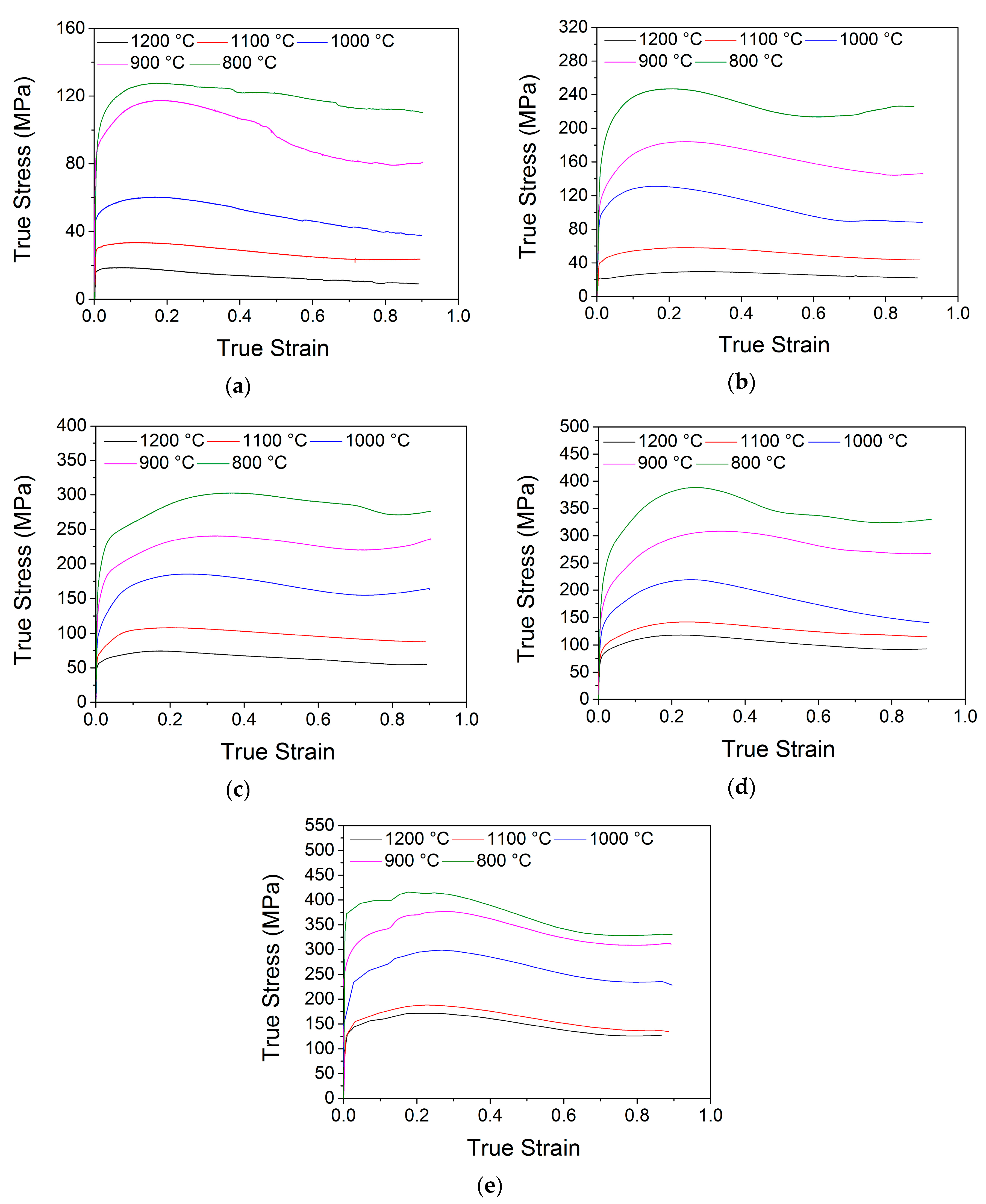
3.1. True Stress–Strain Behavior and Microstructure of X153CrMoV12 Steel

The flow curves of X153CrMoV12 steel at different temperatures and strain rates are displayed in Figure 5. All curves show a rapid increase in the flow stress due to a pronounced work hardening in the first phase of compression [20,21]. It is also noticeable that the flow stress decreases with an increase in temperature or with a decrease of deformation rate due to a dynamic recovery (DRV). This effect was also observed in Reference [22]. It is clear that all curves have a single peak stress in the range of 0–0.9% deformations, which is a consequence of dynamic recrystallization (DRX). The peak stresses were obtained for all flow curves in a deformation range of 0.1–0.3%. When peak stress is reached, true stress decreases with increasing deformation due to softening mechanisms [23]. In case of higher temperatures (1100–1200 °C ), it can be stated that there has been reached a balance between softening and hardening mechanisms and the steady state stress has been achieved from deformations above 0.5%. Moreover, in temperature range of 800–1000 °C in the deformation’s region of about 0.6–0.7%, the hardening mechanism again begins to prevail, resulting in a slight rise of the flow curves.

The microstructure of the selected samples refers to the limiting temperature conditions and the deformation rates in Figure 6. In the case of low deformation temperatures (800 °C) and strain rates of 0.001 s⁻¹ and 10 s⁻¹, there was no structural change in the samples compared to the base material, since the austenization of the selected material only occurs above A_C1 = 820 °C and finishes with A_C3 = 850 °C (Figure 6a,b). The resulting structure was formed by a ferritic matrix with several large primary and small secondary carbides. It is known that the energy in the form of heat is released by deformation of the atomic lattice. This generated heat did not play any important role due to the fact that the welded thermocouples on the sample detected this change and immediately cooled the sample to the selected temperature.

In the case of high deformation temperatures (1200 °C), the anisotropy of the microstructure and its difference between the core and the surface of the test specimen occurred (Figure 6c–f). This phenomenon was observed at both low (0.001 s⁻¹) and high strain rate (10 s⁻¹), respectively. The cause is DRX, which occurred in the given temperature in combination with the stress distribution in the deformed body. Since the used experimental sample had small dimensions, there is no presumption of a significant temperature difference between its surface and core during cooling.

After high temperature deformation of the experimental sample, the stress lines have a cylindrical shape. The greatest proportion of deformation and consequently the stress concentration occurs around the surface of the deformed body and decreases towards the core. As a result of DRX, at the temperature T = 1200 °C, distinct polygonal ferritic grains are formed in the core of the samples and the carbides present are deposited at ferritic grain boundaries. In accordance with the literature, the overall grain size is smaller in the case of the higher deformation rate (Figure 6f). DRX did not occur in the subsurface layers during hot deformation. However, deformation laths are formed in the original austenitic grains, where the subsequent decay of austenite upon cooling nucleates new phases having an irregular, often needle-shaped form with carbides (Figure 6c,e).

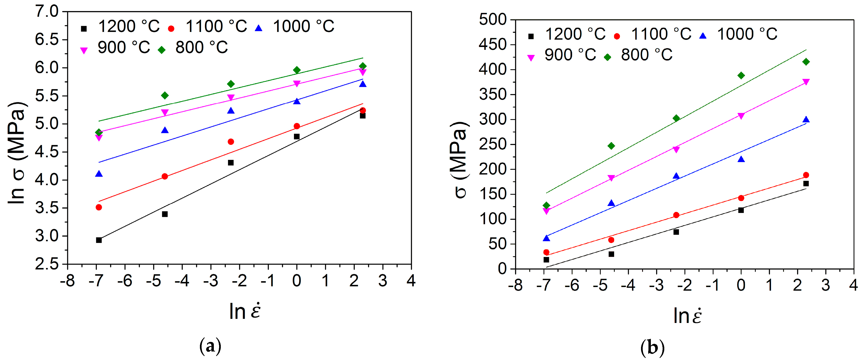
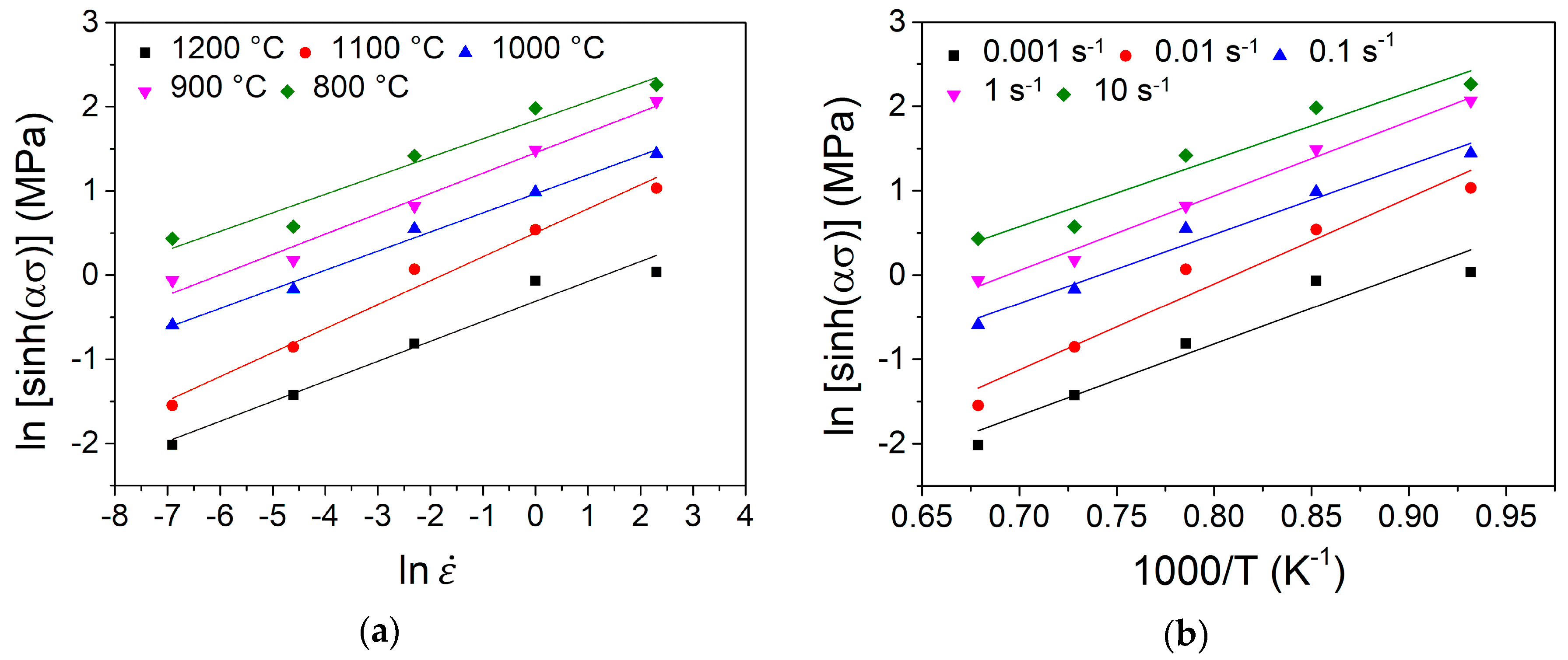
3.2. Constitutive Modelling

The Arrhenius Equation, which is in fact a phenomenological approach, was used to predict constitutive equation [24,25], which gives the flow stress and strain at different temperatures and expresses the Z parameter, known as the Zener–Hollomon parameter [26]. The Z parameter represents the temperature compensated strain rate, which has been widely used to characterize the behavior of materials in hot working [27]. The Z parameter is formulated as:

$$Z=\dot{\epsilon }\exp \left(\frac{Q}{RT}\right)$$

(1)

where $\dot{\epsilon }$ is the strain rate, T is the temperature in K, R is the gas constant (R = 8.314 J·mol⁻¹·K⁻¹) and Q is the activation energy. The strain rate can be expressed:

$$\dot{\epsilon }=A\mathrm{F}\left(\sigma \right)\exp \left(-\frac{Q}{RT}\right)$$

(2)

where

$$\mathrm{F}\left(\sigma \right)=\{\begin{array}{cc}{\sigma }^{n^{\prime }}& \alpha \sigma <0.8\\ \exp \left(\beta \sigma \right)& \alpha \sigma >1.2\\ {\left[\sin \mathrm{h}\left(\alpha \sigma \right)\right]}^n& \mathrm{for} \mathrm{all} \sigma \end{array}$$

(3)

Here, A, n′, β, α and n are the material constants. These constants can be directly determined from experimental data obtained by the hot compression test. The calculation procedure to obtain the material constants for the peak stress will be given in the following section. For the low flow stress level ($\alpha \sigma <0.8$) and the high stress level ($\alpha \sigma >1.2$), the relationship between the flow stress and strain rate can be expressed as the power law and exponential law of $\mathrm{F}\left(\sigma \right)$ in Equation (2), respectively. The correlation between low and high stress can be as follows:

$$\dot{\epsilon }=B{\sigma }^{n^{\prime }}\hspace{1em}(\mathrm{for} \alpha \sigma <0.8)$$

(4)

$$\dot{\epsilon }=B^{\prime } \exp \left(\beta \sigma \right)\hspace{1em}(\mathrm{for} \alpha \sigma >1.2)$$

(5)

where B and B′ are material constants independent from the deformation temperature. After logarithm in Equations (4) and (5) one obtains:

$$\ln \left(\sigma \right)=\frac{1}{n^{\prime }}\ln \left(\dot{\epsilon }\right)-\frac{1}{n^{\prime }}\ln \left(B\right)$$

(6)

$$\sigma =\frac{1}{\beta }\ln \left(\dot{\epsilon }\right)-\frac{1}{\beta }\ln \left(B^{\prime }\right)$$

(7)

Based on Equations (6) and (7), it is possible to determine the parameter n′ and β from the graphical dependencies $\ln \left(\sigma \right)$ vs. $\ln \left(\dot{\epsilon }\right)$ and $\sigma$ vs. $\ln \left(\dot{\epsilon }\right)$, substituting for the stress values the peak stress values of the respective strain rates and temperatures. Then, the parameters will be defined as:

$$n^{\prime }={\left[\frac{\partial \ln \dot{\epsilon }}{\partial \ln \sigma }\right]}_T$$

(8)

$$\beta ={\left[\frac{\partial \ln \dot{\epsilon }}{\partial \sigma }\right]}_T$$

(9)

The value of the parameter n′ is obtained as the reciprocal value of the slope in the $\ln \left(\sigma \right)$ vs. $\ln \left(\dot{\epsilon }\right)$ plot (Figure 7a) and the parameter β as the reciprocal value of the slope in the $\sigma$ vs. $\ln \left(\dot{\epsilon }\right)$ (Figure 7b). It is obvious from the graphical dependencies, that the respective points can be linearly fitted, whereby fitting the lines for individual temperatures have a similar slope. Subsequently, the mean peak stress values will be determined as the average values of the slopes, which are supposed to be temperature independent, namely n′ = 6.343 and β = 0.0451. Consequently, the α parameter is α = β/n′ = 0.00711.

For all stress levels (low and high), Equation (2) can be represented as follows:

$$\dot{\epsilon }=A{\left[\sin \mathrm{h}\left(\alpha \sigma \right)\right]}^n\exp \left(-\frac{Q}{RT}\right)$$

(10)

Logarithming Equation (10), the following equation can be obtained:

$$\ln \left[\sinh \left(\alpha \sigma \right)\right]=\frac{\ln \dot{\epsilon }}{n}+\frac{Q}{nRT}-\frac{\ln A}{n}$$

(11)

By differentiating Equation (11) at constant temperature, it can be written:

$$\frac{1}{n}=\left[\frac{\partial \ln \left[\sinh \left(\alpha \sigma \right)\right]}{\partial \ln \left(\dot{\epsilon }\right)}\right]$$

(12)

where the value of n is again determined as the reciprocal value of the average values of the slopes of the linear fitting in the graphical dependence $\ln \left[\sinh \left(\alpha \sigma \right)\right]$ vs. $\ln \left(\dot{\epsilon }\right)$ for each temperature (Figure 8a) and its value is n = 4.1633. According to Equation (10), for given deformation rates, it is possible to construct the graphical dependencies $\ln \left[\sinh \left(\alpha \sigma \right)\right]$ vs. $1000/T$ (Figure 8b). The slopes of the individual linear fittings form $Q/Rn$ values and thus the hot deformation activation energy values Q can be determined. Its average value is 305.84 kJ/mol. For comparison, in the study of Choudhary [28], the energy for austenitic stainless steel was determined to be Q = 206 kJ/mol and for the magnesium alloy in study of Dong [29] the value was Q = 156.14 kJ/mol, respectively. Both activation energies were associated with the peak stress.

From this graphical dependency $\ln [\sinh \left(\alpha \sigma \right)]$ vs. $\ln \left(\dot{\epsilon }\right)$, the parameter lnA can also be derived from the intercept of the linear fitting according to:

$$\ln A=\frac{Q}{RT}+\frac{C^{\prime }}{n}$$

(13)

where parameter C′ represents the intercepts of the linear fitting for each temperature. Using this approach, the lnA parameter for the respective temperature is obtained and their mean value is lnA = 29.472. Subsequently, using Equation (1), the Zener–Hollomon parameter and peak flow stress value can be expressed taking into consideration Equation (10):

$${\mathsf{\sigma }}_p=\frac{1}{\alpha }\left\{{\left(\frac{\dot{\epsilon } \exp \left(\frac{Q}{RT}\right)}{A}\right)}^{\frac{1}{n}}+{\left[{\left(\frac{\dot{\epsilon } \exp \left(\frac{Q}{RT}\right)}{A}\right)}^{\frac{2}{n}}+1\right]}^{\frac{1}{2}}\right\}$$

(14)

Similar to the material parameters for peak stresses, these parameters can also be determined for the entire strain range. In this case, all of the parameters were calculated for the strain from 0.1 to 0.8 with the step of 0.05. In order to predict the flow stress over a wide range of temperatures and strains, it is necessary to interpolate the obtained values by a certain continuous function. Strain-dependent material parameters are most often translated by a polynomial curve of a certain degree [30,31]. To select the polynomial degree correctly, we fitted obtained points by the polynomials from the 2nd to 7th order and based on the quality of fitting, represented by the coefficient of determination R², the final decision for an appropriate equation selection could be made. Figure 9 shows the graph of the parameter R² depending on the polynomial order. It can be seen that the polynomial of third order is sufficient to determine the α and n parameters correctly (Figure 9a,b), since at higher polynomial the fitting accuracy increased negligibly. For the parameters Q and lnA (Figure 9c,d) it is necessary to apply a polynomial fitting of fifth order to obtain sufficient fitting accuracy. Finally, the material parameters can be expressed using the following equations (polynomial fitting constants are listed in

Table 3. Polynomial fitting constants of parameters α, n, Q, and lnA for X153CrMoV12 steel.

Parameter α F1(ε)	Parameter n F2(ε)	Parameter Q F3(ε)	Parameter lnA F4(ε)
D0 = 0.00865	E0 = 4.68845	F0 = 345.97489	G0 = 29.20644
D1 = −0.01197	E1 = −4.13312	F1 = −584.199	G1 = −56.96311
D2 = 0.03589	E2 = 6.57538	F2 = 2959.985	G2 = 288.41427
D3 = −0.02392	E3 = −3.57347	F3 = −7346.774	G3 = −719.18308
-	-	F4 = 8897.969	G4 = 871.30332
-	-	F5 = −4048.710	G5 = −395.7832

):

$$\alpha =D_0+D_1\epsilon +D_2{\epsilon }^2+D_3{\epsilon }^3$$

(15)

$$n=E_0+E_1\epsilon +E_2{\epsilon }^2+E_3{\epsilon }^3$$

(16)

$$Q=F_0+F_1\epsilon +F_2{\epsilon }^2+F_3{\epsilon }^3+F_4{\epsilon }^4+F_5{\epsilon }^5$$

(17)

$$\ln A=G_0+G_1\epsilon +G_2{\epsilon }^2+G_3{\epsilon }^3+G_4{\epsilon }^4+G_5{\epsilon }^5$$

(18)

In Figure 10, it can be seen the evolution of individual material parameters depending on the true strain in the range from 0.1 to 0.8. It is obvious from the polynomial fitting that the strain has a significant influence on the evolution of the parameters and when predicting the true stress during hot deformation, it is necessary to use the functional dependence of these parameters, not just a specific value. After determining the material parameters using functional equations, it is possible to express the Arrhenius Equation (14) for different strain and temperature values as follows:

$$\sigma =\frac{1}{{\mathrm{f}}_1\left(\epsilon \right)}\left\{{\left(\frac{\dot{\epsilon } \exp \left(\frac{{\mathrm{f}}_3\left(\epsilon \right)}{RT}\right)}{\exp \left[{\mathrm{f}}_4\left(\epsilon \right)\right]}\right)}^{\frac{1}{{\mathrm{f}}_2\left(\epsilon \right)}}+{\left[{\left(\frac{\dot{\epsilon } \exp \left(\frac{{\mathrm{f}}_3\left(\epsilon \right)}{RT}\right)}{\exp \left[{\mathrm{f}}_4\left(\epsilon \right)\right]}\right)}^{\frac{2}{{\mathrm{f}}_2\left(\epsilon \right)}}+1\right]}^{\frac{1}{2}}\right\}$$

(19)

where the values of ${\mathrm{f}}_{\mathrm{i}}\left(\epsilon \right)$ represent the individual polynomial functions of the material parameters depending on the applied strain.

4. Discussion

A comparison of the measured data with the data obtained by the constitutive model is shown in Figure 11. The present comparison was carried out for the deformation rates from 0.001 s⁻¹ to 10 s⁻¹ and deformation temperatures from 800 °C to 1200 °C. It is noticeable that in case of a deformation rate of 0.001 s⁻¹ at 800 °C, the difference between the measured and the predicted data is relatively large. This can also be observed for a strain rate of 10 s⁻¹ at the same temperature of 800 °C. The differences in these cases are in range from 20 to 80 MPa. In other conditions, the experimental and predicted data are in relative good agreement with deviation up to 20 MPa.

For an overall assessment of the applicability of the given constitutive model for X153CrMoV12 steel, the Pearson’s correlation coefficient R was calculated for the flow stress values at all deformation rates and temperatures by the following equation:

$$R=\frac{E\left\{\left[{\sigma }_E-E\left({\sigma }_E\right)\right]\left[{\sigma }_M-E\left({\sigma }_M\right)\right]\right\}}{{\delta }_x{\delta }_y}$$

(20)

where E denotes the expected value of flow stress, ${\sigma }_E$ and ${\sigma }_M$ experimental and predicted flow stress, respectively, ${\delta }_x$ and ${\delta }_y$ represent the standard deviation of flow stresses. The correlation dependence between measured and predicted flow stress is shown in Figure 12. The value of the correlation coefficient, at which it is enabled to evaluate the possibility of using constitutive model, is R = 0.98267.

As shown, the above procedure for obtaining material constants into the constitutive model based on Zener–Hollomon parameter can also be used in the case of high-strength steel X153CrMoV12. This model can predict flow stress in a relatively large range of deformation rates and temperatures. The boundaries where the model already shows large differences with experimental data are very low deformation rates (≈0.01 s⁻¹) or large deformation rates (≈10 s⁻¹) at deformation temperatures of about 800 °C. This may be related to the fact that these parameters do not cause any structural changes in the material. Therefore, it can be said that this model is better suited for the conditions where the materials undergo microstructural changes.

The flow curves of the investigated material exhibit clear signs of DRX. This was also confirmed by the microstructural examination of this material, where coarse martensitic laths were formed in a temperature range from 1000 °C to 1200 °C after cooling, as opposed to significant grain refinement at lower temperatures in a range of 800–1000 °C.

Variations and inaccuracies were caused by the inaccuracy of the model itself, the linear fitting of the material constants. The change in material structure also had a significant impact, since the stress–strain relationship is a function of the grain size [32]. In other areas of deformation and temperature, the model is relatively well correlated with experimental data, thus, determining the interval at which the model is applicable. Another indicator of the suitability of the model for this material is the fact that the material parameters could be approximated by the polynomial function of the third or the fifth order, respectively, while in other works polynomial functions of the sixth or the seventh order had to be applied [33,34].

5. Conclusion

In this work, hot deformation behavior of X153CrMoV12 steel was investigated at deformation temperatures from 800 °C to 1200 °C and strain rates from 0.001 s⁻¹ to 10 s⁻¹. Constructed flow curves were evaluated using a constitutive model based on the Zener–Hollomon parameters.

The following conclusions can be drawn from the present work:

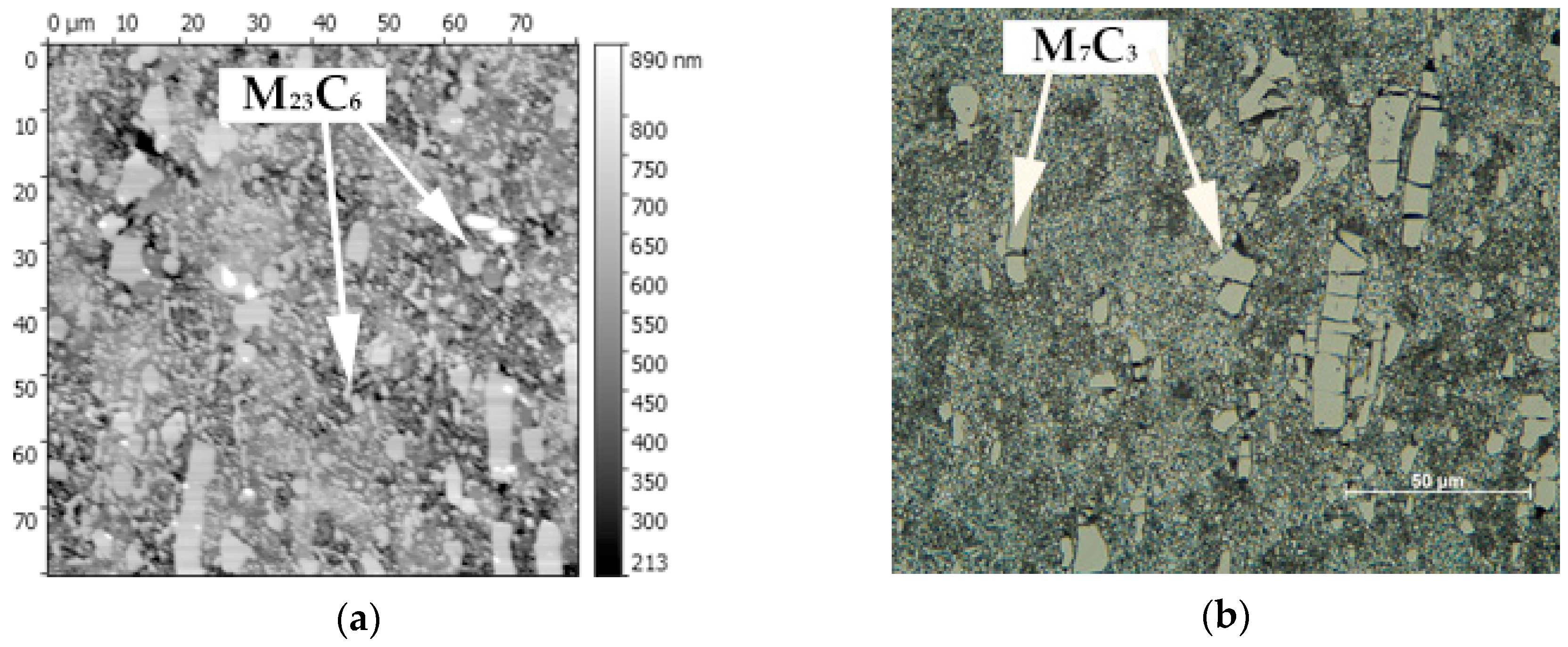
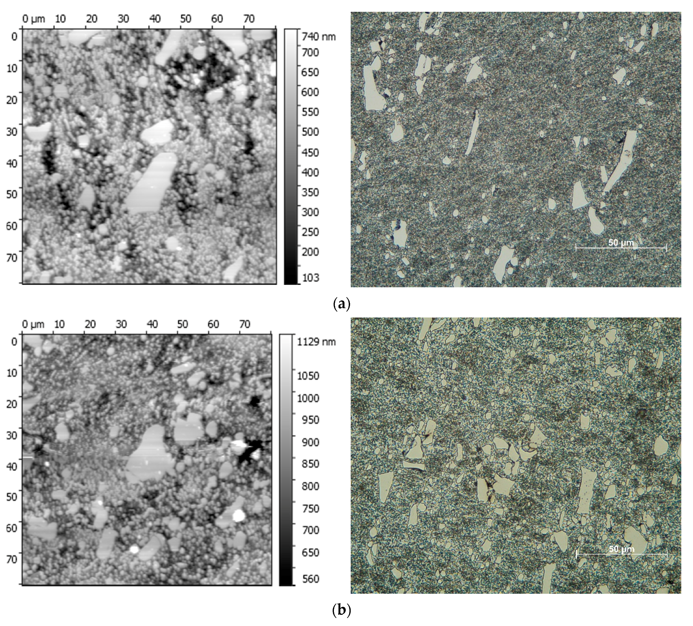
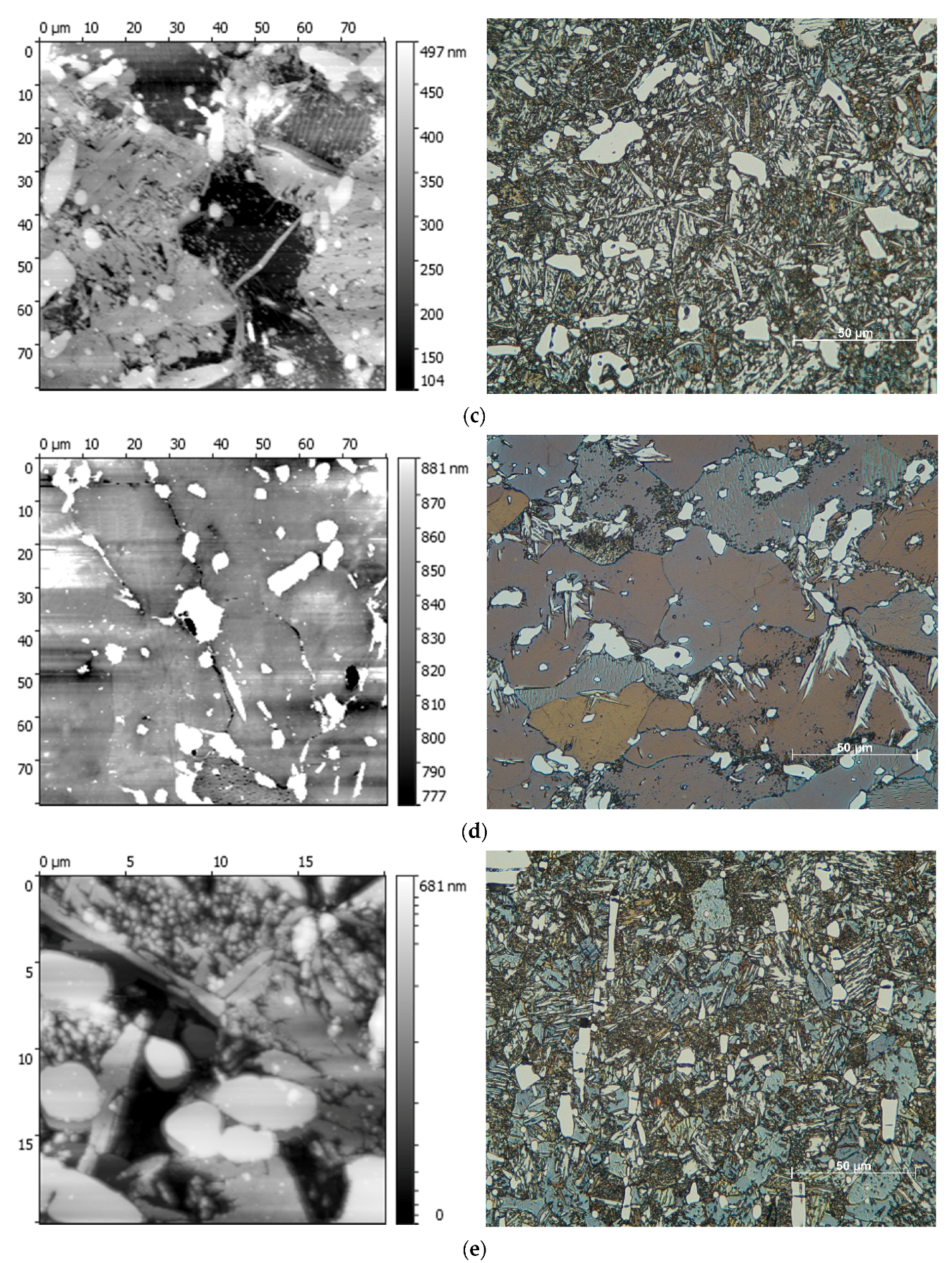
• The microstructure of X153CrMoV12 steel in normalized condition consists of a mixture of coarse M₇C₃ and fine M₂₃C₆ carbides embedded in a ferritic matrix. This microstructure also persisted at low deformation temperatures (T = 800 °C) due to annealing and deformation below critical transformation temperatures.
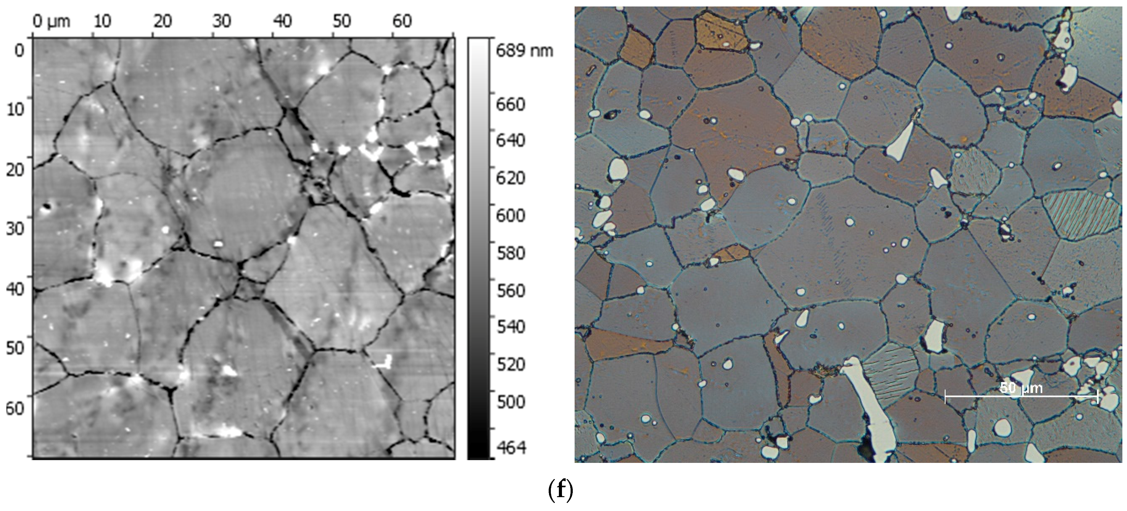
• High deformation temperature (T = 1200 °C) triggered microstructural changes due to the preceding phase transformations and DRX. As a result, the final microstructure had a polygonal ferritic matrix with the carbides deposited at the grain boundaries. In addition, an increase of deformation rate resulted in the obvious grain refinement as an aftermath of proceeding DRX.
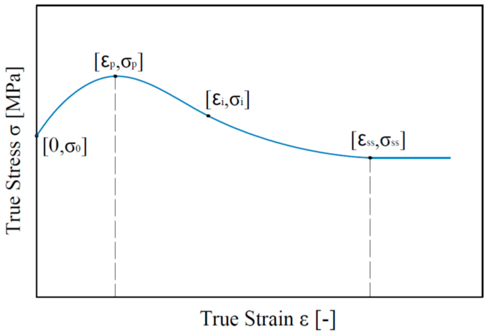
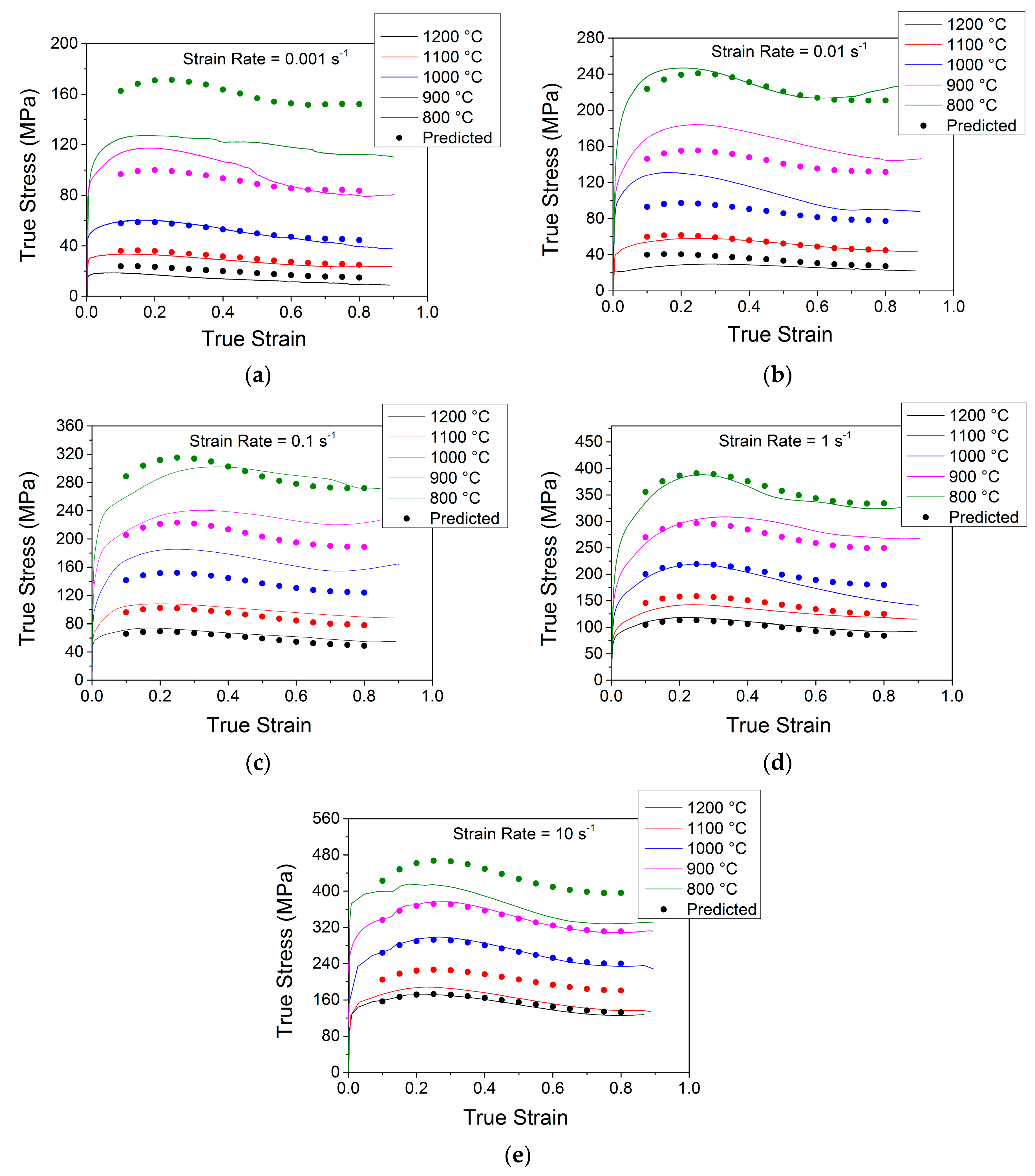
• X153CrMoV12 steel exhibits DRX with a single peak stress in the entire range of temperatures and deformation rates. When peak stress is reached, softening mechanisms start to prevail, which at higher deformation temperatures, balanced with the hardening mechanisms. Finally, the steady state stress stabilizes the flow stress. In case of lower temperatures, where the peak stress is also significant, there is also a significant DRX process in play. Therefore, a significantly refined structure could be observed using both the AFM as well as the LOM technique.
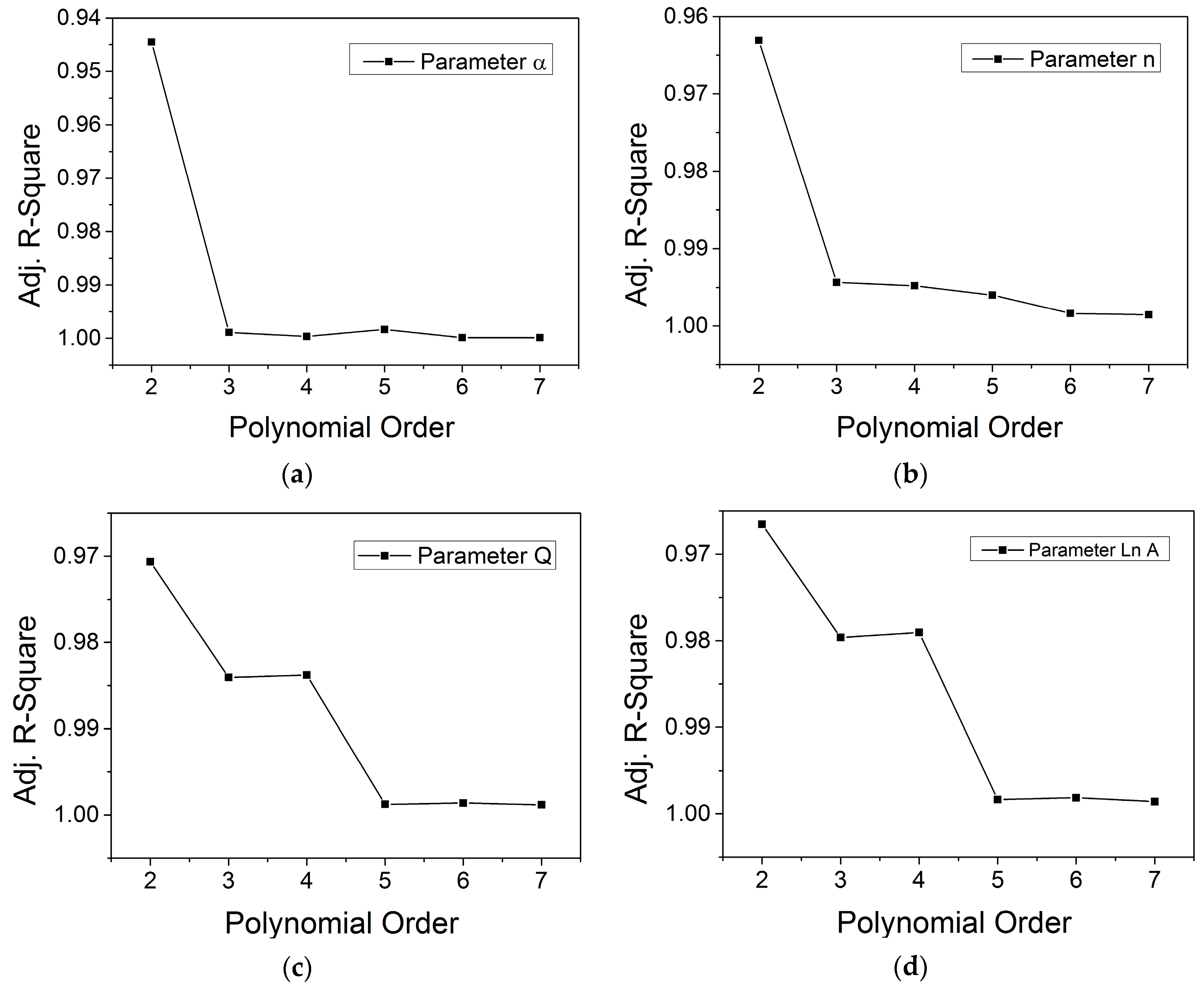
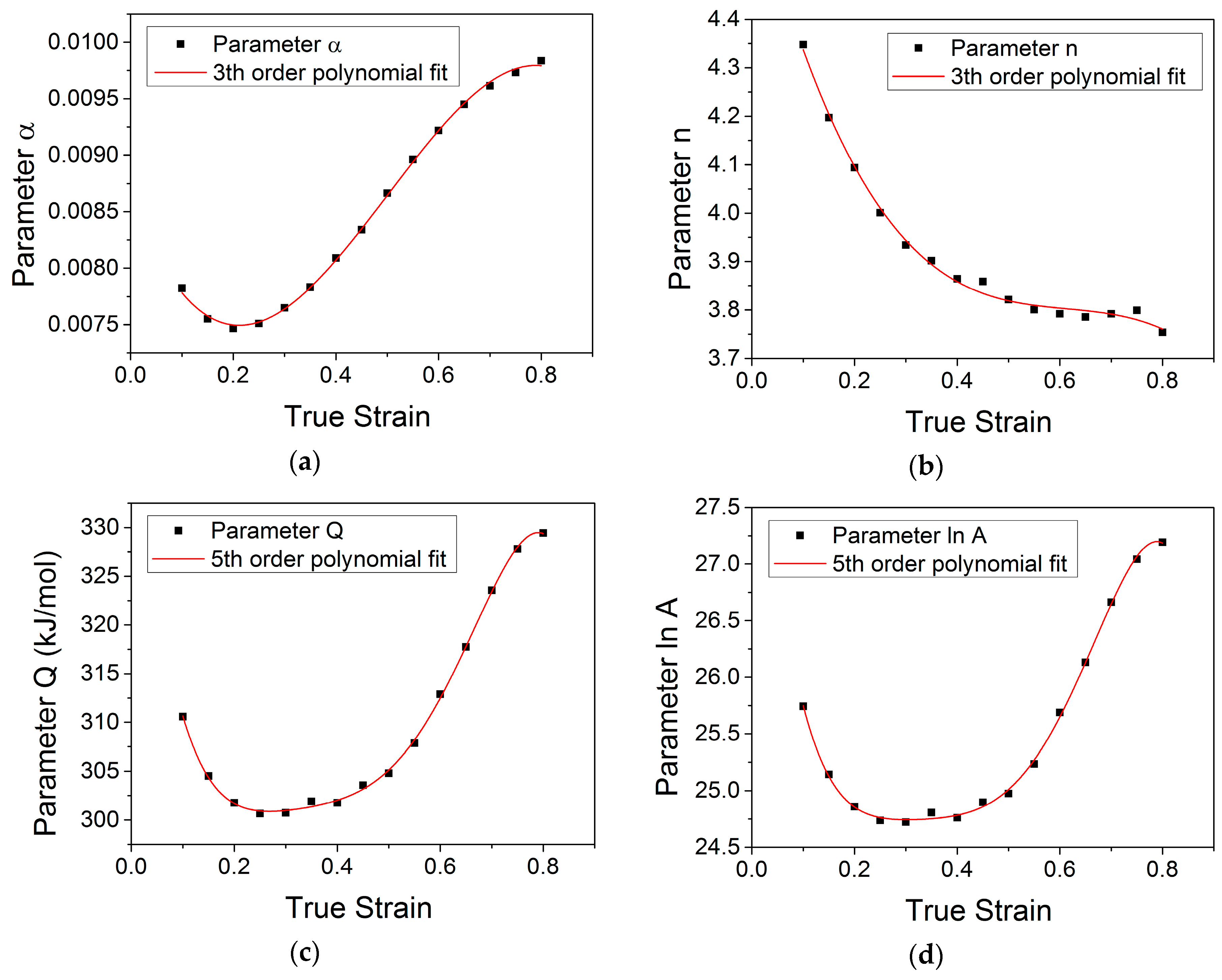
• With constitutive model and flow curves it is possible to obtain material parameters and thus predict true stress and strain behavior in a wide range of temperatures and deformation rates. Material parameters can be obtained by polynomial fitting of the third and fifth order, respectively, which also preserves a certain physical meaning of the parameters while maintaining relative mathematical simplicity.
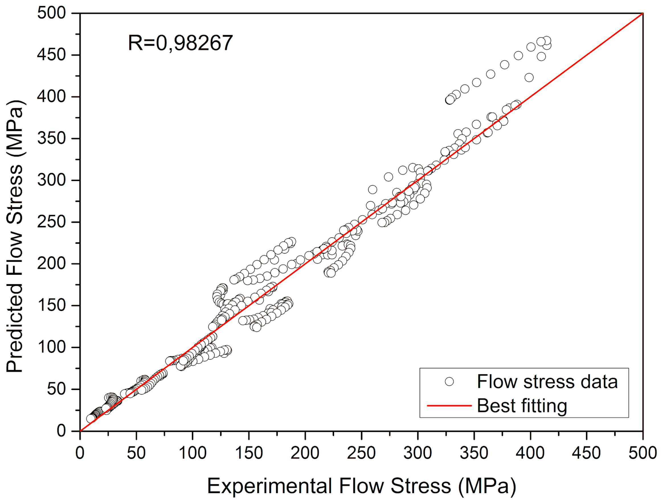
• The flow stress prediction using the above procedure is in relatively good agreement with the experimental flow stress patterns obtained with the correlation coefficient of R = 0.98267. Such a result, along with a graphical comparison of predicted and measured flow stress patterns, allows the use of a constitutive model for predicting the flow curves during hot deformation for these types of high-strength steels.

References

1. Pernis, R.; Kasala, J.; Bořuta, J. High temperature plastic deformation of CuZn30 brass-calculation of the activation energy. Kov. Mater. 2010, 48, 41–46. [Google Scholar] [CrossRef]
2. Garofalo, P. An Empirical Relationship Defining the Stress Dependence of Minimum Creep Rate in Metals. Trans. Metall. Soc. AIME 1963, 227, 351–355. [Google Scholar]
3. Sellars, C.M.; Tegart, W.J. Hot Workability. Int. Metall. Rev. 1972, 17, 1–24. [Google Scholar] [CrossRef]
4. Lenard, J.G. Modelling Hot Deformation of Steels: An Approach to Understanding and Behaviour, 1st ed.; Springer: Berlin/Heidelberg, Germany; New York, NY, USA, 1989; pp. 1–33. [Google Scholar]
5. Bai, D.Q.; Yue, S.; Sun, W.P.; Jonas, J.J. Effect of deformation parameters on the no-recrystallization temperature in Nb-bearing steels. Metall. Trans. A 1993, 24A, 2151–2159. [Google Scholar] [CrossRef]
6. Maccagno, T.M.; Jonas, J.J.; Yue, S.; McCrady, B.J.; Slobodian, R.; Deeks, D. Determination of Recrystallization Stop Temperature from Rolling Mill Logs and Coparison with Laboratory Simulation Results. ISIJ Int. 1994, 34, 917–922. [Google Scholar] [CrossRef]
7. Spigarelli, S.; Cabibbo, M.; Evangelista, E.; Bidulská, J. A study of the hot formability of an Al-Cu-Mg-Zr alloy. J. Mater. Sci. 2003, 38, 81–88. [Google Scholar] [CrossRef]
8. Solhjoo, S. Analysis of flow stres sup to the peak at hot deformation. Mater. Des. 2009, 30, 3036–3040. [Google Scholar] [CrossRef]
9. Ptačinová, J.; Sedlická, V.; Hudáková, M.; Dlouhý, I.; Jurči, P. Microstructure—Toughness relationship in sub-zero treated and tempered Vanadis 6 steel compared to conventional treatment. Mater. Sci. Eng. A 2017, 702, 241–258. [Google Scholar] [CrossRef]
10. Yang, J.; Cao, B.; Wu, Y.; Gao, Z.; Hu, R. Continuous cooling transformation (CCT) behavior of a high Nb-containing TiAl alloy. Materialia 2019, 5, 100169. [Google Scholar] [CrossRef]
11. Sobotova, J.; Jurci, P.; Dlouhy, I. The effect of subzero treatment on microstructure, fracture toughness, and wear resistance of Vanadis 6 tool steel. Mater. Sci. Eng. A 2016, 652, 192–204. [Google Scholar] [CrossRef]
12. Jurči, P.; Dománková, M.; Hudáková, M.; Ptačinová, J.; Pašák, M.; Palček, P. Characterization of microstructure and tempering response of conventionally quenched, short- and long-time sub-zero treated PM Vanadis 6 ledeburitic tool steel. Mater. Charact. 2017, 134, 398–415. [Google Scholar] [CrossRef]
13. Fischmeister, H.F.; Riedl, R.; Karagöz, S. Solidification of high-speed tool steels. Metall. Trans. A 1980, 20, 2133–2148. [Google Scholar] [CrossRef]
14. Hetyner, D.W. Refining carbide size distributions in M1 high speed steel by processing and alloying. Mater. Charact. 2001, 46, 175–182. [Google Scholar] [CrossRef]
15. Kheirandish, S. Effect of Ti and Nb on the formation of carbides and the mechanical properties in As-cast AISI-M7 high-speed steels. ISIJ Int. 2001, 41, 1502–1509. [Google Scholar] [CrossRef]
16. Pirtovšek, T.V.; Kugler, G.; Godec, M.; Terčelj, M. Microstructural characteritation during the hot deformation of 1.17C-11.3Cr-1.48V-2.24W-1.35Mo ledeburitic tool steel. Mater. Charact. 2011, 62, 189–197. [Google Scholar] [CrossRef]
17. Valloton, J.; Herlach, D.; Henein, H. Effect of convection on the dendride groeth kinetics in undercooled melts of D2 tool steels. IPO Conf. Ser. Mater. Sci. Eng. 2016, 117, 012058. [Google Scholar] [CrossRef]
18. Hunkel, M.; Surm, H.; Steinbacher, M. Dilatometry. In Handbook of Thermal Analysis and Calorimetry; Vazovkin, S., Koga, N., Schick, C., Eds.; Elsevier: Amsterdam, The Netherlands, 2018; Volume 6, pp. 103–129. [Google Scholar]
19. Berkowski, L. The influence of warm plastic deformation on the structure and on the applicable properties of high speed steel. J. Mater. Process. Technol. 1996, 60, 637–641. [Google Scholar] [CrossRef]
20. Lan, L.; Zhou, W.; Misra, R.D.K. Effect of hot deformation parameters on flow stress and microstructure in a low carbon microalloyed steel. Mater. Sci. Eng. A 2019, 756, 18–26. [Google Scholar] [CrossRef]
21. Jha, J.S.; Toppo, S.P.; Singh, R.; Tewari, A.; Mishra, S.K. Flow stress constitutive relationship between lamellar and equiaxed microstructure during hot deformation of Ti-6Al4V. J. Mater. Process. Technol. 2019, 270, 216–227. [Google Scholar] [CrossRef]
22. McQueen, H.J.; Yue, S.; Ryan, N.D.; Fry, E. Hot working characteristic of steels in austenitic state. J. Mater. Process. Technol. 1995, 53, 293–310. [Google Scholar] [CrossRef]
23. Solhjoo, S.; Vakis, A.I.; Pei, Y.T. Two phenomenological models to predict the single peak flow stress curves up to the peak during hot deformation. Mech. Mater. 2017, 105, 61–66. [Google Scholar] [CrossRef] [Green Version]
24. Jiang, L.; Fuguo, L.; Jun, C. Constitutive Model Prediction and Flow Behavior Considering Strain Response in the Thermal Processing for the TA15 Titanium Alloy. Materials 2018, 11, 1985. [Google Scholar] [CrossRef]
25. Samantaray, D.; Mandal, S.; Bhaduri, A.K. A comparative study on Johnson Cook, modified Zerilli-Armstrong and Arrhenius-type constitutive models to predict elevated temperature flow behaviour in modified 9Cr-1Mo steel. Comput. Mater. Sci. 2009, 47, 568–576. [Google Scholar] [CrossRef]
26. Zener, C.; Hollomon, J.H. Effect of Strain Rate upon Plastic Flow of Steel. J. Appl. Phys. 1944, 15, 22–32. [Google Scholar] [CrossRef]
27. Shang, X.; Cui, Y.; Fu, M.W. A ductile fracture model considering stress state and Zener-Hollomon parameter for hot deformation of metallic materials. Int. J. Mech. Sci. 2018, 144, 800–812. [Google Scholar] [CrossRef]
28. Choudhary, B.K. Activation energy for serrated flow in type 316L(N) austenitic stainless steel. Mater. Sci. Eng. A 2014, 603, 160–168. [Google Scholar] [CrossRef]
29. Dong, Y.; Zhang, C.; Lu, X.; Wang, C.; Zhao, G. Constitutive Equations and Flow Behavior of an As-Extruded AZ31 Magnesium Alloy Under Large Strain Condition. J. Mater. Eng. Perform. 2016, 25, 2267–2281. [Google Scholar] [CrossRef]
30. Wei, G.; Peng, X.; Hadadzedeh, A.; Mahmoodkhani, Y.; Xie, W.; Yang, Y.; Wells, M.A. Constitutive modelling of Mg-9Li-3Al-2Sr-2Y at elevated temperatures. Mech. Mater. 2015, 89, 241–253. [Google Scholar] [CrossRef]
31. Li, J.; Gao, B.; Tang, S.; Liu, B.; Liu, Y.; Wang, Y.; Wang, J. High temperature deformation behavior of carbon-containing FeCoCrNiMn high entropz alloy. J. Alloys Compd. 2018, 747, 571–579. [Google Scholar] [CrossRef]
32. Ammouri, A.H.; Kridli, G.; Ayoub, G.; Hamade, R.F. Relating grain size to the Zener-Hollomon parameter for twin-roll-cast AZ31B alloy refined by friction stir processing. J. Mater. Process. Technol. 2015, 222, 301–306. [Google Scholar] [CrossRef]
33. Wang, J.; Liu, Y.; Liu, B.; Wang, Y.; Cao, Y.; Li, T.; Zhou, R. Flow behavior and microstructures of powder metallurgical CrFeCoNiMo0.2 high entropy alloy during high temperature deformation. Mater. Sci. Eng. A 2017, 689, 233–242. [Google Scholar] [CrossRef]
34. Lin, Y.C.; Chen, M.S.; Zhong, J. Constitutive modeling for elevated temperature flow behavior of 42CrMo steel. Comput. Mater. Sci. 2008, 42, 470–477. [Google Scholar] [CrossRef]
Figure 1. Typical high temperature true stress–strain response under compression.
Metals 09 01125 g001
Figure 2. Phase diagram of Fe-Fe3C binary system [9].
Metals 09 01125 g002
Figure 3. Initial microstructure of the X153CrMoV12 steel in normalized condition observed by (a) atomic force microscopy (AFM) and (b) light optical microscopy (LOM).
Metals 09 01125 g003
Figure 4. Calculated phase diagram for X153CrMoV12 steel [14].
Metals 09 01125 g004
Figure 5. True stress–strain curves of high-strength steel X153CrMoV12 under different strain rates, (a) ε ˙ = 0.001 s−1, (b) ε ˙ = 0.01 s−1, (c) ε ˙ = 0.1 s−1, (d) ε ˙ = 1 s−1, (e) ε ˙ = 10 s−1
Metals 09 01125 g005
Figure 6. Microstructure of specimens obtained by AFM (left) and LOM (right): (a) temperature 800 °C, strain rate 0.001 s−1, (b) temperature 800 °C, strain rate 10 s−1, (c) temperature 1200 °C, strain rate 0.001 s−1 (near the outer surface), (d) temperature 1200 °C, strain rate 0.001 s−1 (in the middle), (e) temperature 1200 °C, strain rate 10 s−1 (near the outer surface), (f) temperature 1200 °C, strain rate 10 s−1 (in the middle).
Metals 09 01125 g006aMetals 09 01125 g006bMetals 09 01125 g006c
Figure 7. (a) Relationship between ln ( σ ) and ln ( ε ˙ ) for derivation of n′ parameter, (b) relationship between σ vs. ln ( ε ˙ ) for derivation of β parameter.
Metals 09 01125 g007
Figure 8. (a) Relationship between ln [ sinh ( α σ ) ] vs. ln ( ε ˙ ) for obtaining n parameter, (b) relationship between ln [ sinh ( α σ ) ] vs. 1000 / T for obtaining Q parameter.
Metals 09 01125 g008
Figure 9. Accuracy of polynomial fitting of: (a) Parameter α, (b) Parameter n, (c) Parameter Q, (d) Parameter lnA.
Metals 09 01125 g009
Figure 10. Material parameter dependence in full range of strain, (a) Parameter α, (b) Parameter n, (c) Parameter Q, (d) Parameter lnA.
Metals 09 01125 g010
Figure 11. Comparison between measured and predicted flow stresses of X153CrMoV12 steel, (a) ε ˙ = 0.001 s−1, (b) ε ˙   = 0.01 s−1, (c) ε ˙ = 0.1 s−1, (d) ε ˙ = 1 s−1, (e) ε ˙ = 10 s−1.
Metals 09 01125 g011
Figure 12. The correlation between predicted and measured flow stresses for all measurements.
Metals 09 01125 g012