Damage Evolution Due to Extremely Low-Cycle Fatigue for Inconel 718 Alloy

Abstract

This paper evaluates the damage evolution process under extremely low-cycle fatigue (ELCF). The study explores the damage behavior under different stress states. The influence of the multiaxial state of stress on the metal’s life is determined. Two different stress states were examined: (a) axisymmetric and (b) plane-strain. The study is based on the modified Mohr–Coulomb (MMC) ductile fracture criterion that was extended to cover the ELCF regime in a previous research study. Four distinctive geometries are designed to study the effect of different stress states on ELCF life and damage evolution. The damage model is calibrated for life prediction to agree with the ELCF experimental results. The investigation of the damage evolution behavior is dependent on equivalent plastic strain, stress triaxiality, Lode angle, and cyclic loading effect. The damage evolution is extracted from Abaqus finite element simulations and plotted versus the equivalent plastic strain. The damage accumulation shows nonlinear evolution behavior under cyclic loading conditions. SEM images were taken to further study the microscopic failure mechanisms of ELCF.

1. Introduction

Extreme dynamic and fatigue loadings are very common in engineering product designs. For example, during the shutdown and startup operations, engines and machine components are highly susceptible to this type of loading. It commonly causes engines and machine components to fail due to very high strain cyclic loading, referred to as extremely low-cycle fatigue (ELCF). The dynamic cyclic loadings are due to direct fluctuating forces exerted among the machine parts or due to massive vibration within the machine parts. ELCF is also seen in many engineering structures that are exposed to aerodynamic forces. Therefore, predicting, understanding, and evaluating the damage evolution caused by ELCF with a suitable mathematical model is crucial and challenging. The parameters in such a model should consider the complex geometries of the machine parts, the applied loading conditions, and the material properties.

An extended damage accumulation model for ELCF life prediction was developed with the aid of experimental data in Reference [1]. The original modified Mohr–Coulomb (MMC) model was introduced in Reference [2]. Years later, the MMC model was extended to predict ELCF in Reference [1]. Fatigue damage refers to the process of deterioration for engineering parts and components. The damage model parameters are also strongly related to the applied loads [3]. Historically, Kachanov [4] and Rabotnov [5] developed the concept of continuum damage mechanics and described the metal deterioration. In fatigue life prediction, a nonlinear damage model was proposed by Chaboche et al. [6,7]. Later on, Chaudonneret [8] extended the model to capture the effects of different multiaxial loading conditions. Furthermore, the mean hydrostatic pressure relationship with the multiaxial fatigue limit was investigated by Sines [9] and used later by Chaudonneret [8]. Recently, many studies incorporated the nonlinear damage with the critical plane criteria [10,11,12] and with the energy-critical model [13], to predict multiaxial fatigue life. Moreover, fatigue nonlinear damage models have been investigated at room temperature [14,15] and elevated temperatures [16].

This paper aims to predict, understand, and evaluate damage evolution during multiaxial high strain cyclic loading based on experimental results of Inconel 718 undergoing high strain push–pull cyclic loading conditions. This study is based on finite element analysis (FEA) (using Abaqus/Explicit) to examine the damage evolution under different stress states, prior to crack initiation. The paper shows how damage evolution in ELCF, predicted by the extended MMC model, is dependent on (1) equivalent plastic strain (${\overline{\mathsf{\epsilon }}}_{\mathrm{pl}}$), (2) stress triaxiality, (3) Lode angle, and (4) cyclic loading. The stress triaxiality is the hydrostatic pressure (mean stress over Von-Mises stress) where the Lode angle is the third deviatoric stress invariant. The metal-damage behavior during ELCF is also simulated by Abaqus showing that the damage evolution is a nonlinear evolution.

2. Plasticity Model with a Combined Hardening Rule

The plasticity behavior of fully reversed push–pull cyclic loading conditions for Inconel 718 involves a combined material hardening rule. The kinematic hardening model used in this research was proposed by Chaboche in References [17,18] that captures the Bauschinger effect. The Bauschinger effect is caused due to the microstructure deformation by the irreversible dislocation movement along the crystallographic planes that changes the material’s stress-strain characteristics and displaces the yield surface. The model consists of a number of nonlinear back-stresses as in Equation (1). The Chaboche model is a superposition of three Armstrong and Frederick kinematic hardening rules [19]. The three nonlinear back-stress components $(\mathsf{\alpha }={\mathsf{\alpha }}_1+{\mathsf{\alpha }}_2+{\mathsf{\alpha }}_3)$ were calibrated by simulating the stable Inconel 718 hysteresis loop of the force-displacement curve of the smooth round bar specimen (denoted as “R0”) as in Figure 1. The parameters in Equations (1) and (2) are as follows: ${\mathsf{\alpha }}_{\mathrm{i}}$ is the backstress tensor, ${\mathrm{C}}_{\mathrm{i}}$ and ${\mathrm{B}}_{\mathrm{i}}$ are material-dependent constants, and ${\dot{\overline{\mathsf{\epsilon }}}}^{\mathrm{pl}}$ is the accumulated equivalent plastic strain rate as described in Equation (2). The isotropic hardening rule used was the Vocé isotropic strain hardening function in Equation (4). It is a nonlinear isotropic model that describes a yield surface expansion.

$${\dot{\mathsf{\alpha }}}_{\mathrm{i}}={\mathrm{C}}_{\mathrm{i}}{\dot{\mathsf{\epsilon }}}^{\mathrm{pl}}-{\mathrm{B}}_{\mathrm{i}}{\mathsf{\alpha }}_{\mathrm{i}}{\dot{\overline{\mathsf{\epsilon }}}}^{\mathrm{pl}},\hspace{1em}\mathsf{\alpha }={\displaystyle \sum }_{\mathrm{i}=1}^{\mathrm{n}}{\dot{\mathsf{\alpha }}}_{\mathrm{i}},\hspace{1em}\mathrm{where} \mathrm{n}=3,$$

(1)

$${\dot{\overline{\mathsf{\epsilon }}}}^{\mathrm{pl}}=\sqrt{(\frac{2}{3}) {\dot{\mathsf{\epsilon }}}_{\mathrm{ij}}^{\mathrm{pl}}:{\dot{\mathsf{\epsilon }}}_{\mathrm{ij}}^{\mathrm{pl}}}.$$

(2)

The plasticity model with pressure and Lode angle dependencies (referred as the PPL model) proposed by Bai and Wierzbicki [20] (Equation (3)) captures the effect of different stress states during fatigue tests. It should be noted that the term $\left[1-{\mathrm{c}}_{\mathsf{\eta }}(\mathsf{\eta }-{\mathsf{\eta }}_{\mathrm{o}})\right]\left[{\mathrm{c}}_{\mathsf{\theta }}^{\mathrm{s}}+({\mathrm{c}}_{\mathsf{\theta }}^{\mathrm{ax}}-{\mathrm{c}}_{\mathsf{\theta }}^{\mathrm{s}})(\frac{\mathrm{m}+1}{\mathrm{m}})(\mathsf{\gamma }-\frac{{\mathsf{\gamma }}^{\mathrm{m}+1}}{\mathrm{m}+1})\right]$ in Equation (3) is bounded to a range of 0.5 to 2.0 to ensure yield locus convexity. The plasticity model used the Vocé isotropic strain hardening function, Equation (4), where ${\mathsf{\sigma }}_{\mathrm{y}}$ is the yield stress at zero plastic strain, $\mathrm{Q}$ is the maximum strain hardening of the yield surface, and $\mathrm{b}$ is the rate at which the size of the yield surface change [21,22]. All material parameters in Equations (3) and (4) are set in

Table 1. Material properties and parameters used in the plasticity model in Equations (3) and (4).

E, (GPa)	v	σy, (MPa)	Q, (MPa)	b	${\mathbf{c}}_{\mathsf{\eta }}$	${\mathsf{\eta }}_{\mathbf{o}}$	${\mathbf{c}}_{\mathsf{\theta }}^{\mathbf{s}}$	${\mathbf{c}}_{\mathsf{\theta }}^{\mathbf{a}\mathbf{x}}$	m
201	0.283	45.2	100.3	35.435	0.41	0.33	0.867	1.0	0.749

. The plastic flow potential is shown in Equation (5). For more, readers are advised to read References [20,23,24].

$$\mathsf{\sigma }({\mathsf{\epsilon }}_{pl},\mathsf{\eta },\mathsf{\theta })=\mathsf{\sigma }({\overline{\mathsf{\epsilon }}}_{pl})\left[1-c_{\mathsf{\eta }} (\mathsf{\eta }-{\mathsf{\eta }}_o)\right]\left[c_{\mathsf{\theta }}^s+(c_{\mathsf{\theta }}^{ax}-c_{\mathsf{\theta }}^s)(\frac{m+1}{m})(\mathsf{\gamma }-\frac{{\mathsf{\gamma }}^{m+1}}{m+1})\right],$$

(3)

$$\mathsf{\sigma }({\overline{\mathsf{\epsilon }}}_{pl})={\mathsf{\sigma }}_y+Q(1-e^{-b{\overline{\mathsf{\epsilon }}}_{pl}}),$$

(4)

$$f=\sqrt{\frac{3}{2}\left[S-\mathsf{\alpha }\right]:\left[S-\mathsf{\alpha }\right]}-\mathsf{\sigma }({\overline{\mathsf{\epsilon }}}_{pl},\mathsf{\eta },\mathsf{\theta })=0.$$

(5)

3. Measurement of Damage

Material damage in the mechanics of solid materials, i.e., metals and alloys, polymers, composites, concrete, etc., is the study of the creation of the microvoids (or microcracks) and growth, where discontinuities initiate in a continuum material at a larger scale. Physically, ductile damage mechanics is essentially associated with irreversible strains (plastic strains). As damage is introduced to a crack-free material (undamaged metal) during a heavy loading process, many material properties are affected in different manners; a decrease in the elasticity modulus, yield stress, hardness, density, and an increase in the creep strain rate are observed [25,26].

Now, damage due to ELCF (under very high plastic strain amplitudes and high stresses) is physically described as internal micro-stresses that lead to microdecohesions by slip band arrests. The microcracks propagate through either the crystals (grains), known as transgranular, or along the grain boundaries, known as intergranular, depending on the environment, material, and loading conditions. Thus, the extended MMC damage material model (Equations (6) and (7)) predicts ELCF and is capable of modeling the accumulated damage evolution during repeated fully reverse cyclic loading. In the continuum mechanics, the damage is known as the “internal degradation of a continuum solid”. It is represented by $\mathrm{D}$ (see Figure 2a–c) and ranges between $0<\mathrm{D}<1$, where $\mathrm{D}$ = 0 represents a metal with zero flaws whereas $\mathrm{D}$ = 1 represents a fracture initiation occurrence.

$${\overline{\mathsf{\epsilon }}}_{{\mathrm{f}}_{ }}(\mathsf{\eta },\overline{\mathsf{\theta }}){\begin{array}{c}=\left\{\frac{\mathrm{A}}{{\mathrm{c}}_2} \left[{\tilde{\mathrm{c}}}_{\mathsf{\theta }}^{\mathrm{s}}+\frac{\sqrt{3}}{2-\sqrt{3}}({\tilde{\mathrm{c}}}_{\mathsf{\theta }}^{ax}-{\tilde{\mathrm{c}}}_{\mathsf{\theta }}^{\mathrm{s}})(\mathbf{sec}(\frac{\overline{\mathsf{\theta }}\pi }{6})-1)\right]\times \left[\sqrt{\frac{1+ c_1^2}{3}}\mathbf{cos}(\frac{\overline{\mathsf{\theta }}\pi }{6})+c_1(\mathsf{\eta }+\frac{1}{3} \mathbf{sin}(\frac{\overline{\mathsf{\theta }}\pi }{6}))\right]\right\}\end{array}}^{\raisebox{1ex}{$-1$}\!\left/ \!\raisebox{-1ex}{$\mathrm{N}$}\right.}$$

(6)

$$\mathrm{D}=\mathrm{D}({\overline{\mathsf{\epsilon }}}_{\mathrm{pl}})= {{\displaystyle \int }}_0^{{\overline{\mathsf{\epsilon }}}_{\mathrm{pl}}}({\mathrm{c}}_{\mathrm{g}}\mathrm{D}+\frac{{\mathrm{c}}_{\mathrm{g}}}{{\mathrm{e}}^{{\mathrm{c}}_{\mathrm{g}}}-1}).{(1+{\mathrm{c}}_{\mathrm{h}}{ \mathrm{D}}^{{\mathsf{\beta }}_1}{\mathsf{\mu }}^{{\mathsf{\beta }}_2})}^{\mathrm{k}}\frac{\mathrm{d}{\overline{\mathsf{\epsilon }}}_{\mathrm{pl}}}{{\overline{\mathsf{\epsilon }}}_{\mathrm{f}}(\mathsf{\eta },\overline{\mathsf{\theta }})}.$$

(7)

The parameters in Equation (6) ($\mathrm{A}$, $\mathrm{N}$, ${\tilde{\mathrm{c}}}_{\mathsf{\theta }}^{\mathrm{s}}$, ${\tilde{\mathrm{c}}}_{\mathsf{\theta }}^{\mathrm{ax}}$, ${\mathrm{c}}_1$, and ${\mathrm{c}}_2$) are material parameters that are calibrated based on a scripted MATLAB code to match the simulation crack initiation to the experimental one. The first function $({\mathrm{c}}_{\mathrm{g}}\mathrm{D}+\frac{{\mathrm{c}}_{\mathrm{g}}}{{\mathrm{e}}^{{\mathrm{c}}_{\mathrm{g}}}-1})$ in Equation (7) has the parameter ${\mathrm{c}}_{\mathrm{g}}$ that controls the damage evolution behavior as concave or convex (see Figure 3). The second function ${(1+{\mathrm{c}}_{\mathrm{h}}{ \mathrm{D}}^{{\mathsf{\beta }}_1}{\mathsf{\mu }}^{{\mathsf{\beta }}_2})}^{\mathrm{k}}$ incorporates the effect of the different tensor direction between the current stress and the back-stress. This function is activated when reverse loading (non-proportional) exists. The material parameters in both functions (${\mathrm{c}}_{\mathrm{g}},{ \mathrm{c}}_{\mathrm{h}}$, ${\mathsf{\beta }}_1,{ \mathsf{\beta }}_2$, and $\mathrm{k}$) is calibrated under reverse loading tests. The damage model was initially set to predict ductile fracture damage (in Reference [2]) and was extended later in Reference [1] to predict ELCF. The damage model is based on the parameters ${\overline{\mathsf{\epsilon }}}_{\mathrm{pl}}$, η, $\overline{\mathsf{\theta }}$, and $\mathsf{\mu }$ defined as equivalent plastic strain, stress triaxiality, Lode angle, and effect of cycling loading during ELCF, respectively. The state parameters change as the loading process continues and they can be tracked by FEA (using an Abaqus/Explicit user-defined material subroutine). The importance of each parameter in understanding the damage evolution, due to ELCF, is discussed in the following sections. All damage material parameters in Equations (6) and (7) are set in

Table 2. Material parameters used in the modified Mohr–Coulomb (MMC) criterion in Equation (6).

${\mathbf{c}}_1$	${\mathbf{c}}_2 (\mathbf{MPa})$	${\tilde{\mathbf{c}}}_{\mathsf{\theta }}^{\mathbf{s}}$	${\mathbf{c}}_{\mathsf{\theta }}^{\mathbf{a}\mathbf{x}}$	A	N
0.05897	764.587 MPa	0.86277	1	1481	0.0812

and

Table 3. Material of non-proportional parameters used in Equation (7).

${\mathbf{c}}_{\mathbf{g}}$	${\mathbf{c}}_{\mathbf{h}}$	${\mathsf{\beta }}_1$	${\mathsf{\beta }}_2$	$\mathbf{k}$
−6.01	3.0	0.049	0.000001	−1.0

.

3.1. Equivalent Plastic Strain

The first state variable of the four variables in the extended MMC damage model is strain. It is observable, internal, and it is split into elastic strain ${\overline{\mathsf{\epsilon }}}_{\mathrm{el}}$ and plastic strain ${\overline{\mathsf{\epsilon }}}_{\mathrm{pl}}$. The experimental observations of the plastic strain show that the accumulated plastic strain mainly governs the material damage in the form of plane slip along the crystallographic planes and dislocation movements. The accumulated equivalent plastic strain used in this model is defined in agreement with the Von-Mises criterion, ${\dot{\overline{\mathsf{\epsilon }}}}^{\mathrm{pl}}= \sqrt{(\frac{2}{3}) {\dot{\mathsf{\epsilon }}}_{ij}^{pl}:{\dot{\mathsf{\epsilon }}}_{ij}^{pl} }$. Studies show that there is a strong relation between the accumulated plastic deformation, which is represented by the equivalent plastic strain, and the ductile fracture crack formation [27]. The current study investigates the relationship between the accumulated equivalent plastic strain and the damage accumulation during the cyclic loading process.

3.2. Stress Triaxiality Parameter

The dimensionless hydrostatic pressure parameter, termed stress triaxiality $(\mathsf{\eta }={\mathsf{\sigma }}_{\mathrm{H}}/\overline{\mathsf{\sigma }})$, is the hydrostatic stress $({\mathsf{\sigma }}_{\mathrm{H}}=({\mathsf{\sigma }}_1+{\mathsf{\sigma }}_2+{\mathsf{\sigma }}_3)/3)$ over the Von-Mises equivalent stress $(\overline{\mathsf{\sigma }}= \sqrt{3{\mathrm{J}}_2})$. The initial stress triaxiality can be estimated using Bridgman’s analysis for an axisymmetric stress state as in Reference [28] and by the analytical solutions provided in Reference [29] for the plane-strain stress state. High-stress triaxiality zones $(\mathsf{\eta }>1.0)$ can be seen in highly constrained regions such as the center of the notched specimen, or at crack tips. On the other hand, low-stress triaxiality zones $(\mathsf{\eta }<0)$ are often observed where the principal shear stress is considerably higher relative to the hydrostatic stress (i.e., at the surfaces and protruding corners) [27]. Stress triaxiality has been extensively applied in many ductile fracture models [30,31,32,33,34]. Studies show that material ductility depends evidently on the stress triaxiality. The equivalent strain to fracture for numerous ductile materials, over different ranges of strain rates, is also strongly dependent on the stress triaxiality [23,35]. However, quantitative studies of stress triaxiality effects on fatigue life and damage accumulation have not been sufficiently investigated [1,36], yet this area merits extensive consideration. This study focuses on how the damage accumulation due to ELCF is affected by stress triaxiality as part of the fatigue life-prediction model (Equations (6) and (7)).

3.3. Lode Angle Parameter

The Lode angle θ, which is related to the third deviatoric stress invariant, ranges between $0<\mathsf{\theta }<\frac{\mathsf{\pi }}{3}$. The Lode angle can be normalized by the following equation $\overline{\mathsf{\theta }}=1-(6\mathsf{\theta }/\mathsf{\pi })$. Hence, the normalized Lode angle ranges between $-1<\overline{\mathsf{\theta }} <1$. It is used to describe the stress state along with the stress triaxiality. For example, uniaxial tension corresponds to $\overline{\mathsf{\theta }}=1$ and $\mathsf{\eta }=\raisebox{1ex}{$1$}\!\left/ \!\raisebox{-1ex}{$3$}\right.$ whereas pure shear corresponds to $\overline{\mathsf{\theta }}=0$ and $\mathsf{\eta }=0$, and uniaxial compression gives $\overline{\mathsf{\theta }}=-1$ and $\mathsf{\eta }=\raisebox{1ex}{$-1$}\!\left/ \!\raisebox{-1ex}{$3$}\right.$. Any state of $\overline{\mathsf{\theta }}$ other than the above states is a representation of a combined multiaxial stress state (Figure 2d).

3.4. Cyclic Loading Parameter Effect

During cyclic (push–pull) loading, the material experiences a shift in its yield surface. The yield surface moves slightly due to kinematic hardening during each cyclic loading. The center of the yield surface becomes the back-stress coordinate and not the origin. A mathematical model is set to capture the effect of the change in the non-proportional loading direction by measuring the current stress and the back-stress tensors, which is represented by a scalar parameter χ in Equation (8).

$$\mathsf{\chi }= 1- \frac{{\mathsf{\sigma }}_{\mathrm{ij}}:{\mathsf{\alpha }}_{\mathrm{ij}} }{\Vert {\mathsf{\sigma }}_{\mathrm{ij}}\Vert ·\Vert {\mathsf{\alpha }}_{\mathrm{ij}}\Vert },$$

(8)

$$\mathsf{\mu }= {{\displaystyle \int }}_0^{{\overline{\overline{\mathsf{\epsilon }}}}_{\mathrm{pl}}}\mathsf{\chi }\mathrm{d}{\overline{\mathsf{\epsilon }}}_{\mathrm{pl}}.$$

(9)

The range of χ is $\left[0,2\right]$ where χ = 0 means that there is no difference in the direction of the current stress and the back-stress tensors, whereas χ = 2 represents a 180° difference in direction (Figure 4). Another scalar parameter $\mathsf{\mu }$ in Equation (9) is the accumulated differences captured by χ during the cyclic loading process. On the other hand, the parameter $\mathsf{\mu }$ is incorporated in the damage accumulation model Equation (7). To illustrate this, one can see that the parameter χ changes from zero to two in the beginning of a reverse loading, and it reduces to zero after a certain amount of continuing loading. The parameter $\mathsf{\mu }$ keeps increasing if there are changes in the loading path as in Figure 5. The change in loading condition during reverse loading from tension to compression is represented by (i) and (iii) whereas (ii) represents the change from compression to tension in Figure 5.

3.5. Damage Evolution Parameter

The damage evolution parameter ${\mathrm{c}}_{\mathrm{g}}$ in Equation (7) is considered as the critical parameter in simulating the damage evolution under ELCF. The different curves in

Table 4. A comparison of the stress states between the calculations and the finite element analysis (FEA) simulations.

Specimen	Calculations		FEA Simulations
	η	$\overline{\mathsf{\theta }}$	η	$\overline{\mathsf{\theta }}$
R1	0.7423	1.00	0.7623	0.99
R2	0.5105	1.00	0.6165	1.01
PE	0.5774	0	0.6141	0.4530

is for the monotonic loading case. Previously, the material damage evolution due to ELCF has not been studied intensively in terms of knowing the development behavior of the damage accumulation during the cycling loading. The importance of the damage parameter expresses how to simulate the evolution of the material damage and whether it accumulates linearly or nonlinearly. Later in this research, the investigation of the ELCF damage is explained based on this parameter to comprehend the multiaxial ELCF damage evolution thoroughly.

4. Experiments

The specimens’ geometries were designed in a way to confirm that the fatigue occurs at a selected stress state. The calculations to achieve a desired stress states were based on Reference [23] and the computer simulations confirmed the attained stress state by the following two parameters: stress triaxiality and Lode angle (Table 4). For instance, the uniaxial tension stress state had η = 0.333 and $\overline{\mathsf{\theta }}$ = 1 by calculations while the plane strain stress state had η = 0.577 and $\overline{\mathsf{\theta }}$ = 0.

The metal is Inconel 718 (a nickel-based super alloy) and is made in USA (Metalmen Inc., Long Island City, NY, USA) with the chemical composition in wt% shown in

Table 5. Inconel 718 chemical composition as received.

Ni	Cr	Mo	Cb + Ta	N	Si	Cu	Al	C	Mn	Fe
52.86	18.39	2.78	5.09	0.0069	0.079	0.057	0.49	0.039	0.086	Bal.

. This material is widely known in the aerospace and defense industry. It is heavily used in most hot environment applications due to its excellent high strength and fatigue properties at high temperatures. ELCF test series of eight specimens under different high strain amplitudes were executed until specimen full fracture. The cyclic loading hysteresis loops and the strain-life curves are shown in Figure 6 and Figure 7, respectively. The tests strain rate was 0.003/s and the elongation range related to reference gauge length are summarized in

Table 6. Test data and strain measurements.

Specimen Type	Test #	Gauge Length, mm	Elongation Range (%)	Nf
Notched bar with small external radius	1	9	33	4
Notched bar with small external radius	2	9	16	9
Notched bar with large external radius	3	16	33	10
Notched bar with large external radius	4	16	16	41
Notched bar with large external radius	5	16	5	51
Plane-strain	6	4	33	10
Plane-strain	7	4	16	21
Plane-strain	8	4	5	43

.

The servohydraulic testing machine (model 370.10) has a ±100 kN load cell range manufactured by MTS systems corporations^® in Eden Prairie, MN, USA. The force and displacement tests data were concurrently recorded by the loading machine and an optical measurement system, respectively. The optical measurement system measured and recorded the strains during the cyclic loading using a Digital Imaging Correlation (DIC) of type VIC-2D version 5 software made by correlated Solutions Inc^® in Irmo, SC, USA.

4.1. Test Specimen Geometry

Four distinctive shapes were designed in order to study the effect of different stress states on ELCF life and damage evolution. The four shapes were a smooth round bar, small external notch round bar “R0”, large external notch round bar “R1”, and flat plane-strain bar “PE”. A 3D demonstration and detailed dimensions in mm are expressed in Figure 8a,b and

Table 7. Key dimensions and denotation of the four samples.

Specimen Type	Denotation	Notch Radii, (R)	Minimum Diameter, (d) or Thickness (t)	Grips Side Diameter, D
(a) Standard smooth round bar	R0	∞	6.350 mm	12.700 mm
(b) Notched bar with small external radius	R1	3.175 mm	6.350mm	12.700 mm
(c) Notched bar with large external radius	R2	9.525 mm	6.350 mm	12.700 mm
(d) Plane-strain	PE	∞	t = 3.048 mm	12.700 mm

. All specimens were fabricated from one material block to ensure property and microstructure similarity.

4.2. Loading Conditions

The testing machine’s upper grip held the top part of the specimen and remained fixed while the lower grip pulled/pushed the specimen. The fatigue tests were conducted at room temperature. The four shapes of the specimens (Table 7) were designed in such a way to attain different stress states, three of which (R0, R1, and R2) are classified as axisymmetric stress states and one (PE) is classified as a plane-strain stress state. The axisymmetric stress state had two identical principal stresses (${\mathsf{\sigma }}_2= {\mathsf{\sigma }}_3)$ and the Lode angle parameter equals unity ($\overline{\mathsf{\theta }}=1$). The smooth round bar, R0, ($\mathsf{\eta }=1/3$) was used for calibrating the plasticity model (Reference [1]) and the two parameters (A, N) in Equation (6). The sharp notch “R1” and large notch specimens “R2” ($\mathsf{\eta }=0.74 \mathrm{for} “\mathrm{R}1” \mathrm{and} \mathsf{\eta }=0.51 \mathrm{for} “\mathrm{R}2”$) were used to study the effect of the stress triaxiality on the ELCF life, which is clearly demonstrated in the strain–life curve (Figure 7). The plane-strain stress state corresponds to $\overline{\mathsf{\theta }}=0$, and it adds additional important details to be further investigated. By comparing the plane-strain stress state with the axisymmetric stress state, the value of $\overline{\mathsf{\theta }}$ in specimens is different. Consequently, the effect of the Lode angle (or the normalized third stress invariant) on ELCF life can be studied.

5. Damage Evolution Evaluation

In this section, the material damage model for ELCF life prediction is evaluated covering a wide spectrum of fatigue loading conditions (i.e., variable and constant strain amplitude loading, different loading stress states, wide range of different strain ratio, and a wide array of alternating stresses). This damage model shows a suitable explanation of fatigue damage under all the aforementioned complexities in loading conditions and stress states. A quantitative study is described here to expose the complicated underlying ELCF mechanisms throughout the loading process.

5.1. ELCF Damage Evolution

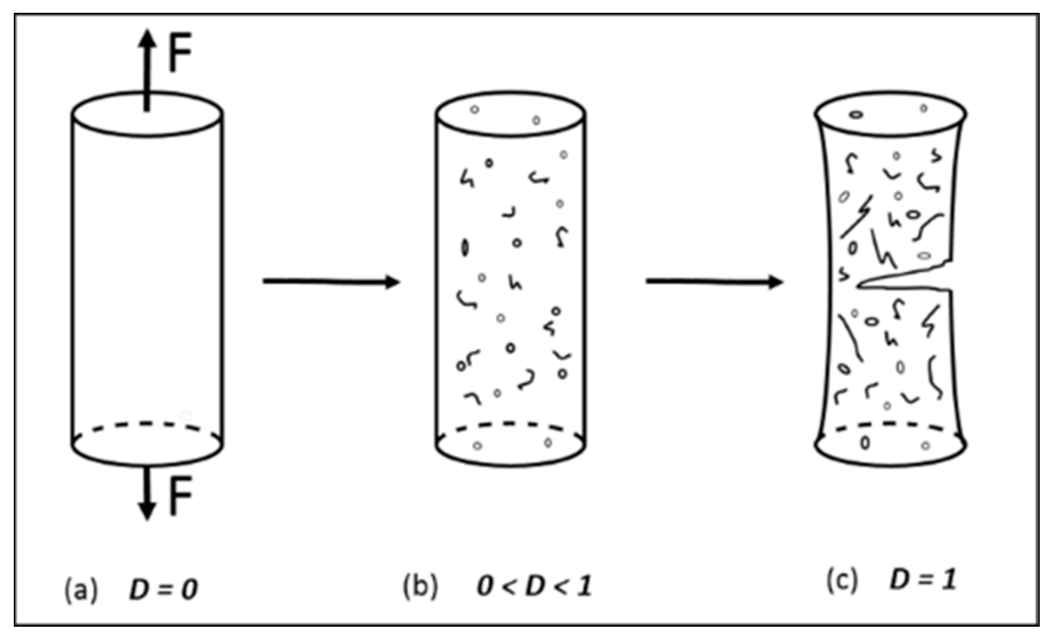
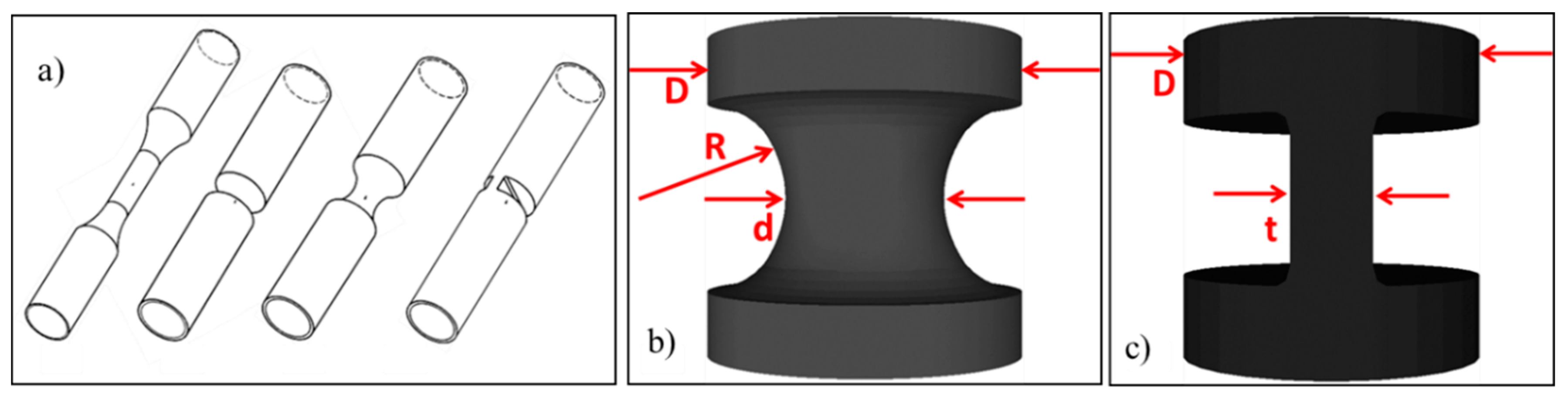
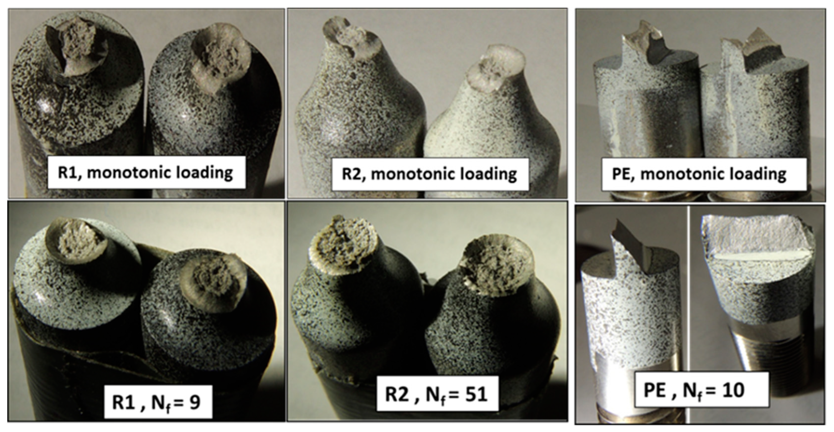
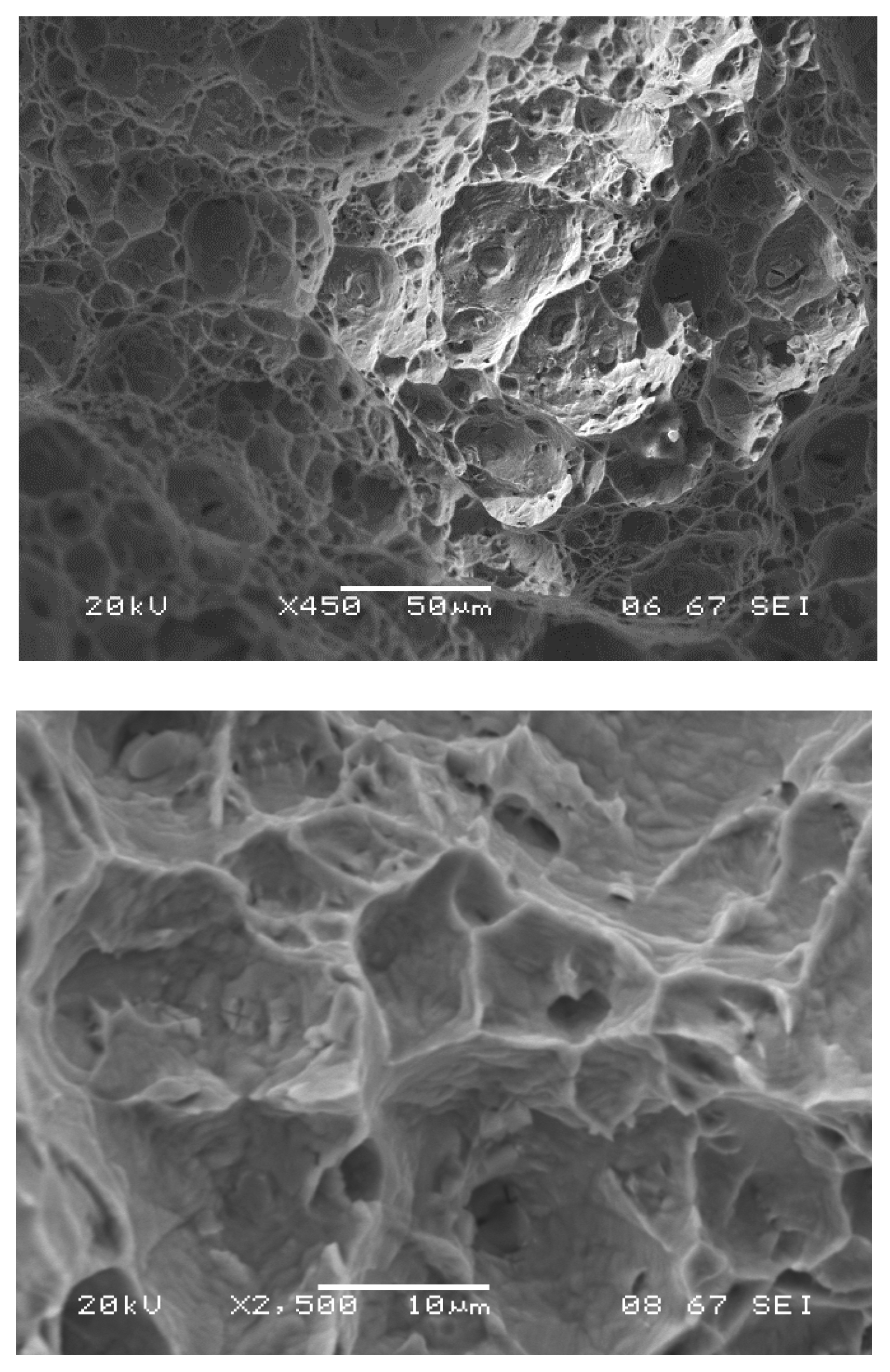
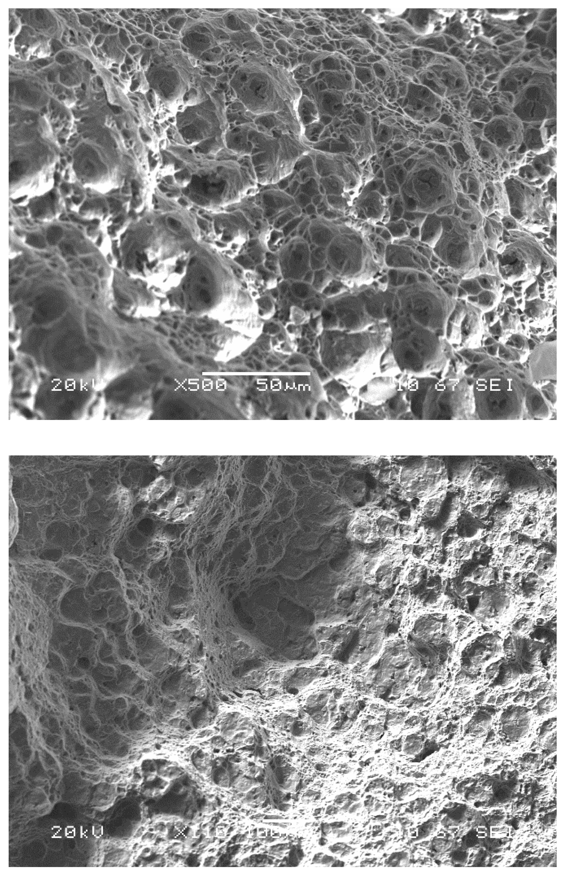
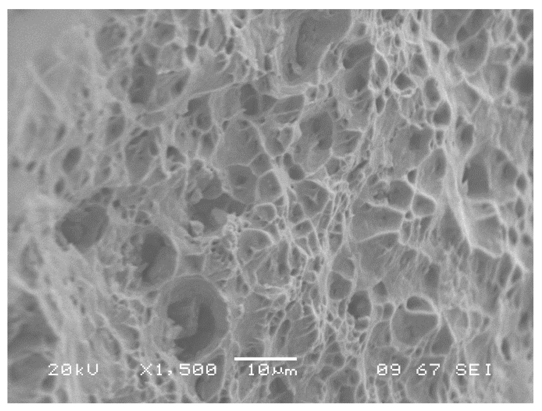
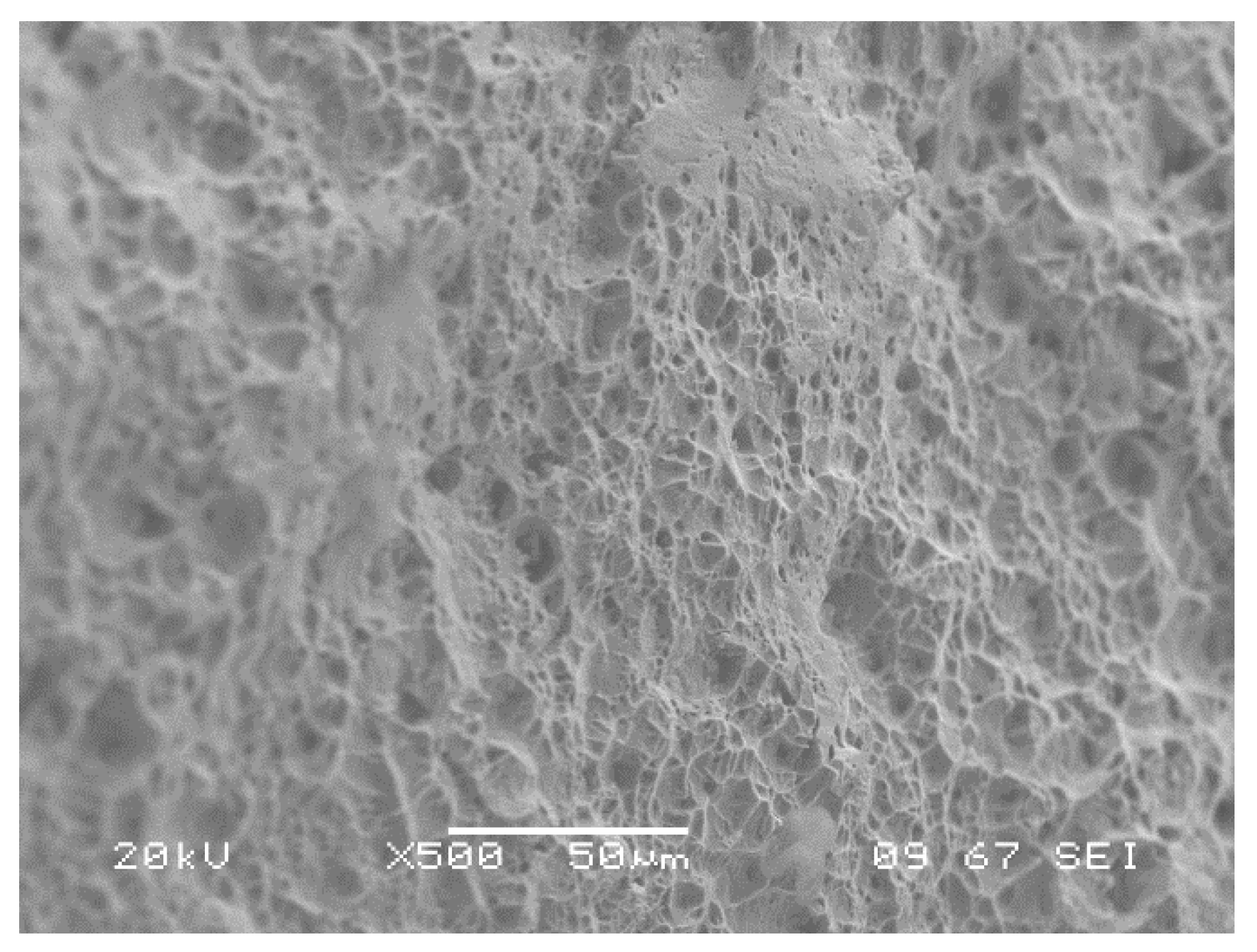
Investigating multiaxial damage evolution due to ELCF can be performed by inspecting three distinguished features on the specimen’s fracture surface: the crack initiation site, the crack growth behavior, and the final fractured surface. Crack initiation likely occurs in highly stressed regions (i.e., microvoids or discontinuities due to a crystallographic plane slip). Crack growth studies the crack propagation rate and crack type: transgranular or intergranular. The specimens’ fractured surface reveals the fracture mode and the grains deformation using SEM. This section will focus on the microstructure damage and damage evolution prior to crack initiation. The ELCF process in the very early loading cycles creates microstructure changes in the bulk of the material and rapidly form strain localization because of the high strain amplitude. The mechanism of the microstructure deformation is caused by the irreversible dislocation movement along the crystallographic planes. As the dislocation pattern in many bundles (veins) becomes localized and the number of persistent slip bands (PSB) increases, the strain localization occurs and forms plastic strain accordingly. A consensus of opinion among researchers is that the PSB are where most cracks initiate in isotropic materials under reverse loading [37]. This explanation of the irreversible damage mechanism is from a microscopic perspective. However, in numerical simulations, the irreversible damage mechanism is quantitatively represented as shown by the accumulated damage $\mathrm{D}$ in Equations (6) and (7). The tendency of the damage evolution behavior during the cycling loading is ambiguous and yet to be discovered. It is not known whether the damage under ELCF accumulates linearly or nonlinearly. In other words, is the damage accumulation rate steady during ELCF or not?

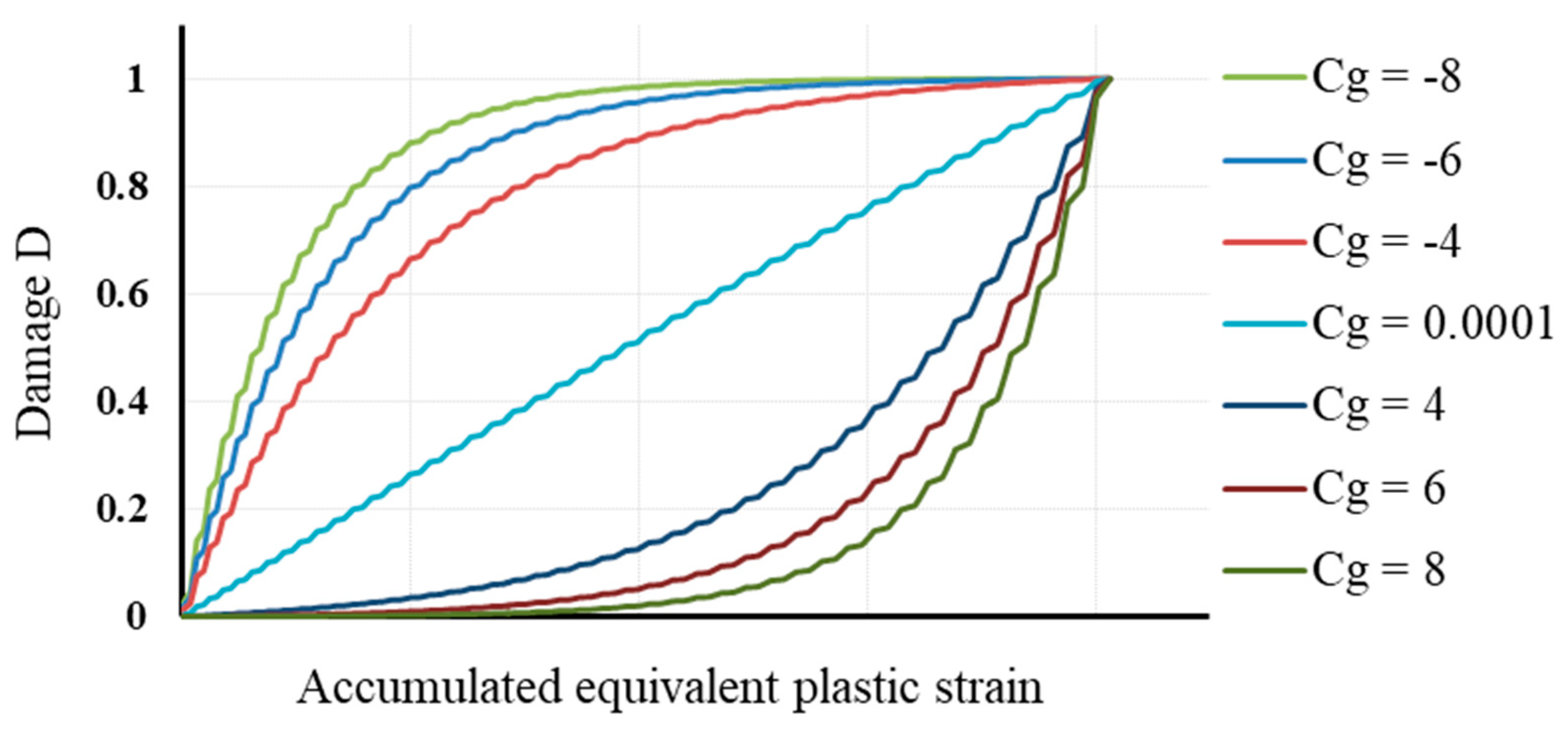
To study the damage accumulation, the parameter ${\mathrm{c}}_{\mathrm{g}}$ in Equation (7) is the focal parameter that will examine the damage evolution behavior under ELCF. For this reason, the damage model (Equations (6) and (7)) was set in a MATLAB code and graphed versus ${\overline{\mathsf{\epsilon }}}_{\mathrm{pl}}$ with a wide range of different ${\mathrm{c}}_{\mathrm{g}}$ values, $-8<{\mathrm{c}}_{\mathrm{g}}<8$ (Figure 3). 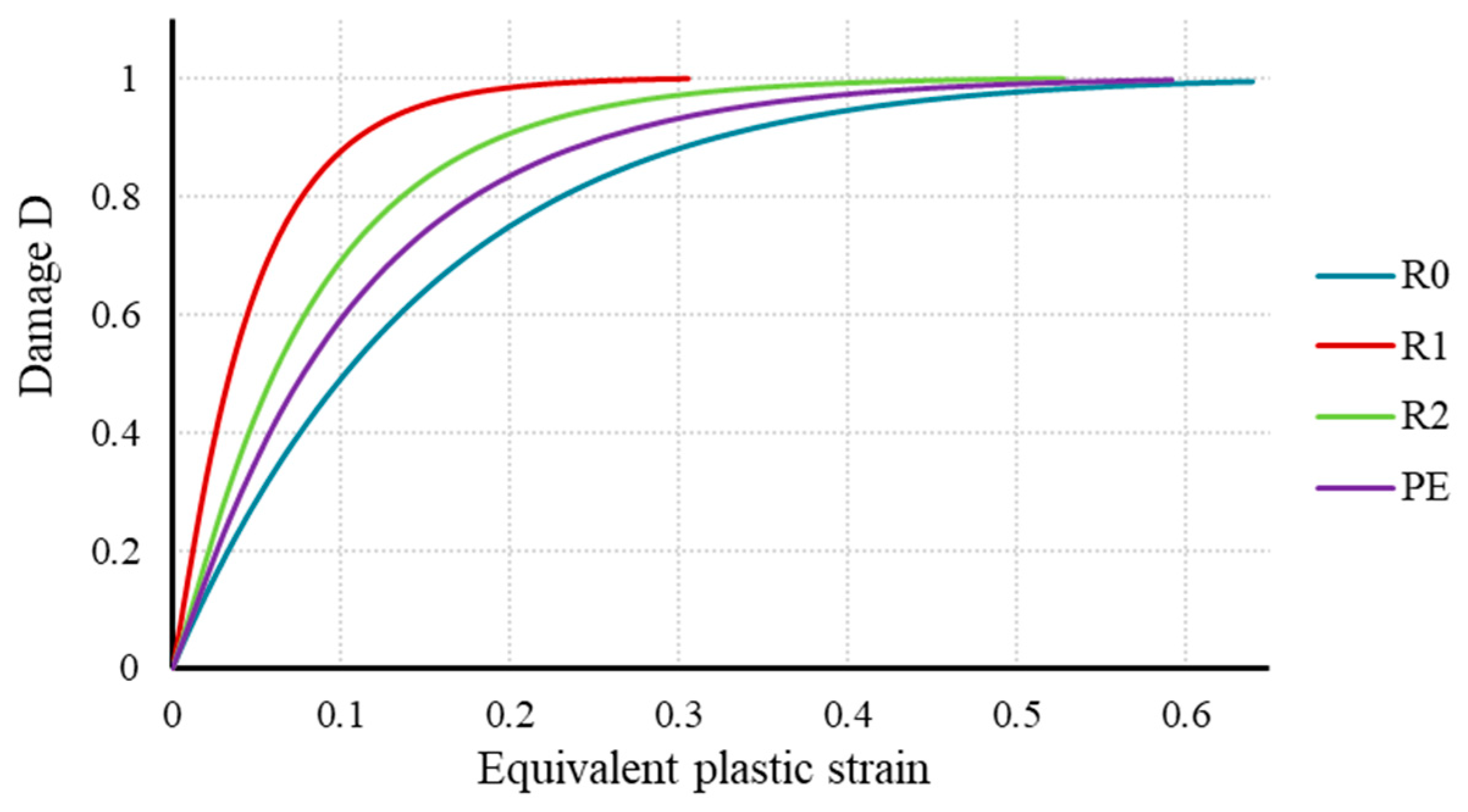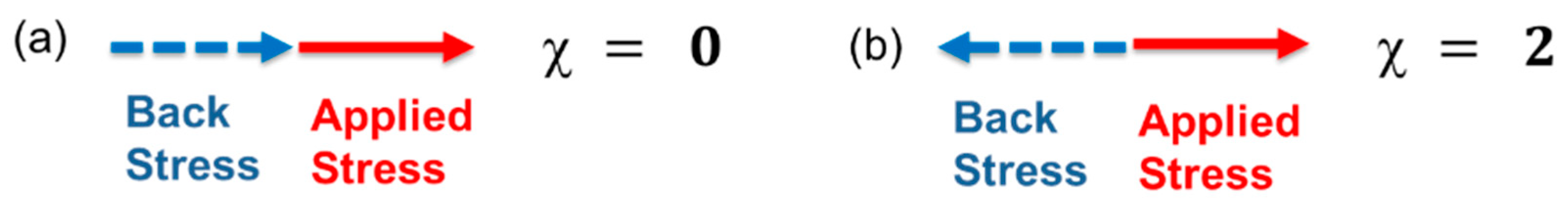The various values of ${\mathrm{c}}_{\mathrm{g}}$ makes the damage evolution behave differently where $\mathrm{D}$ may behave linearly or nonlinearly. In other words, the damage $\mathrm{D}$ evolution is predicted in FEA by the parameter ${\mathrm{c}}_{\mathrm{g}}$. Thus, the damage $\mathrm{D}$ may have multi-evolution trends: linear when ${\mathrm{c}}_{\mathrm{g}}$ is approaching to zero (i.e., ${\mathrm{c}}_{\mathrm{g}}=0.0001$), nonlinear concave curve when ${\mathrm{c}}_{\mathrm{g}}<0$, and nonlinear convex curve when ${\mathrm{c}}_{\mathrm{g}}>0$ (all different evolution trends are depicted in Figure 3). It is worth noting that a nonzero (${\mathrm{c}}_{\mathrm{g}}\ne 0$) should be set to avoid mathematical singularity in the model.

On the other hand, damage evolution due to cycling loading was seen to behave differently. In Reference [1], a good prediction of ELCF life, using Equation (7), was obtained when ${\mathrm{c}}_{\mathrm{g}}<0$. The fatigue life prediction shows good agreement with the experimental results. Hence, the damage accumulation of the specimen’s life under monotonic loading becomes nonlinear (Figure 9) and is in good agreement with the experiment results. Accordingly, the new unified model introduced in Reference [1] predicts both ductile fracture and ELCF.

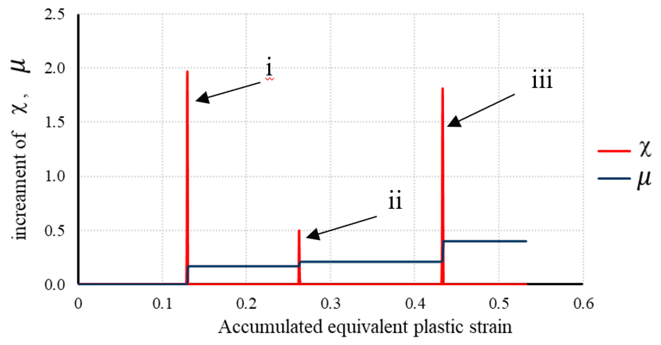
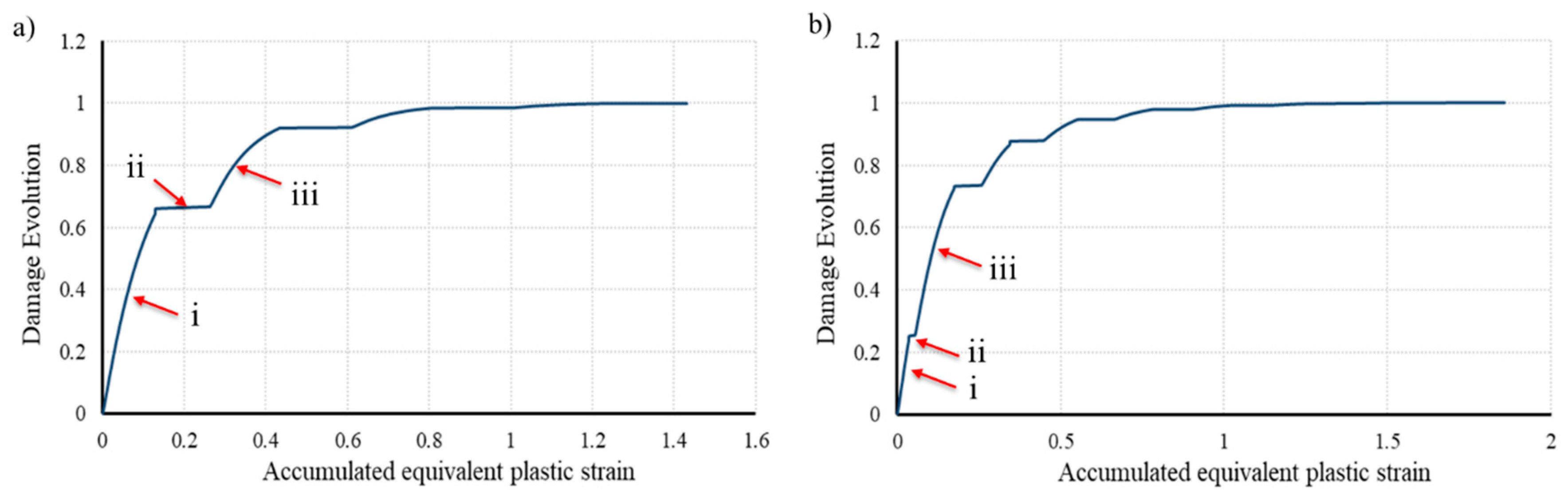
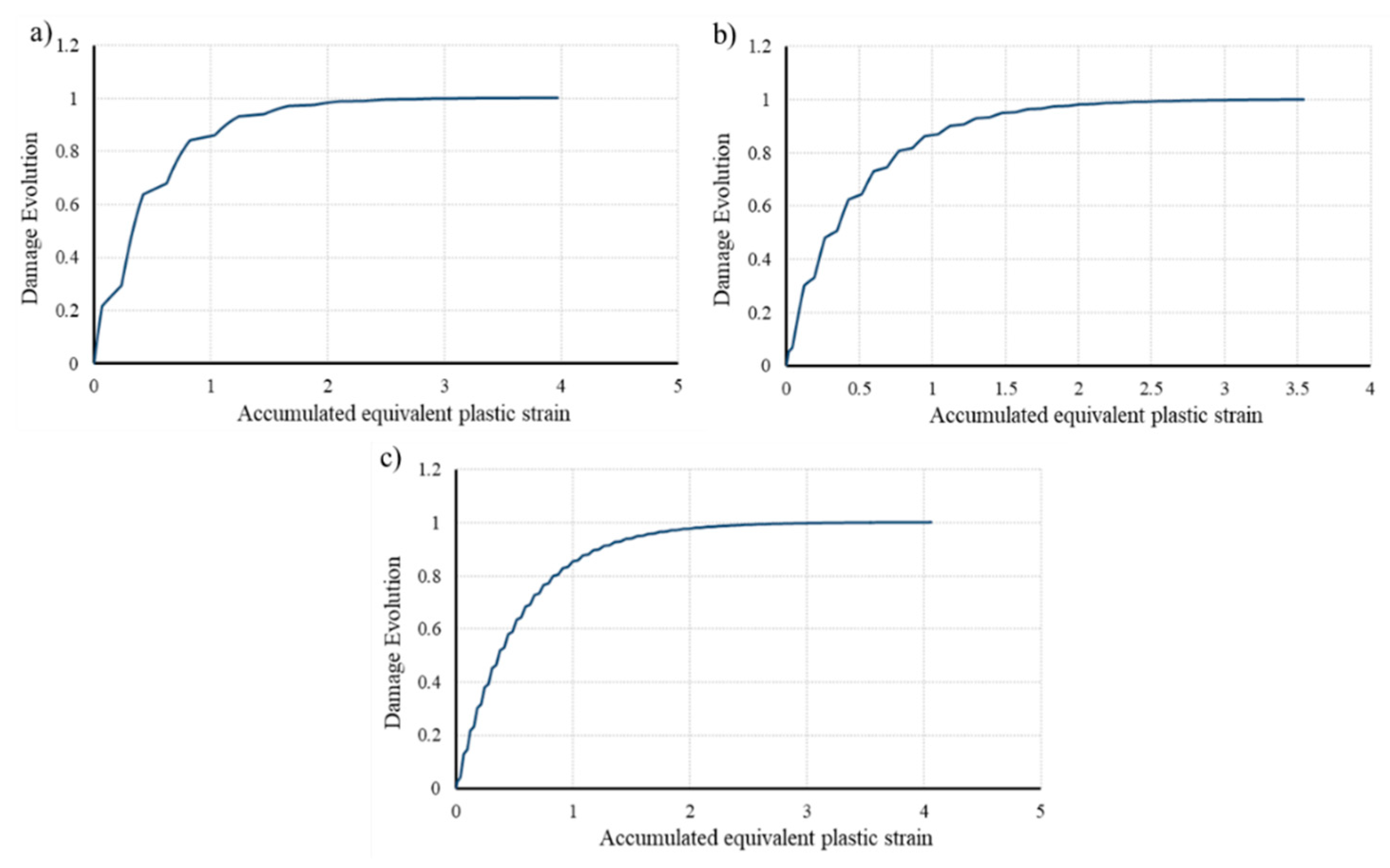
The damage evolution during the high strain cyclic loading for the two “R1” specimens, in the FEA, was seen to increase rapidly in the first couple of cycles until the accumulated equivalent plastic strain reaches around 0.5. Afterwards, the damage evolution starts to accumulate slowly as the cycling process continues. This slow evolution in damage becomes even slower as the specimen reaches its life limit. In Figure 10a, the specimen fails due to fatigue at four high-strain reversed cycles (reminder: the failure occurs when damage accumulation reaches unity). During the first reversed cycle, the damage evolves from zero to approximately 0.67 as the equivalent plastic strain reaches 0.12. In the second cycle, the damage accumulation evolves to about 0.90 as the equivalent plastic strain reaches 0.45. During cycles 3 and 4, the damage accumulation slightly increases to 0.97 and 1, respectively. Similarly, Figure 10b simulates a similar damage evolution behavior for nine high-strain reversed cycles. The end of the curve line represents the fatigue full failure (D = 1).

In Figure 10a,b, the damage evolution during the tension loading in the first cycle is represented by (i). Similarly, damage evolution during the tension loading in the second cycle is represented by (iii), whereas the damage evolution during the compression loading in the first cycle is represented by (ii). It is seen that the damage evolution during compression loading is very small (≈0.0001) and almost negligible. The same applies for the remaining number of reverse loading cycles.

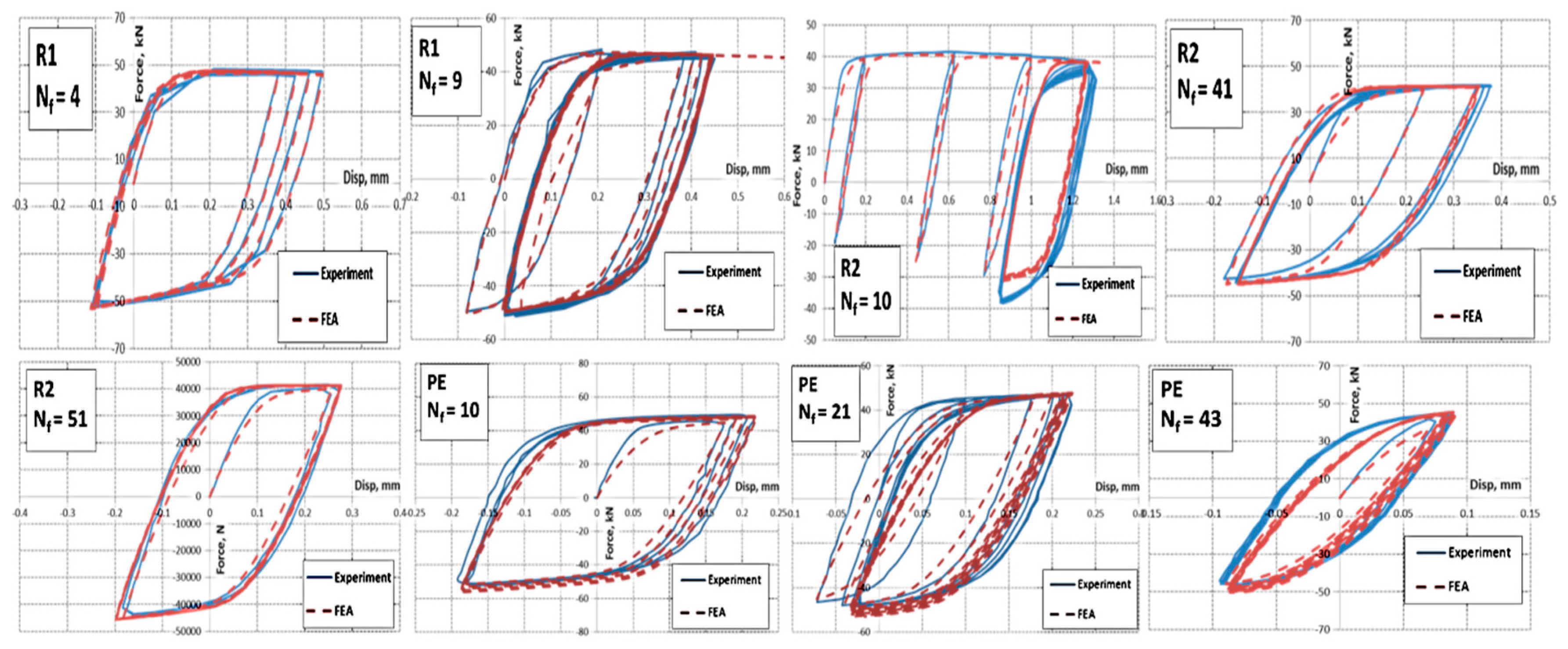
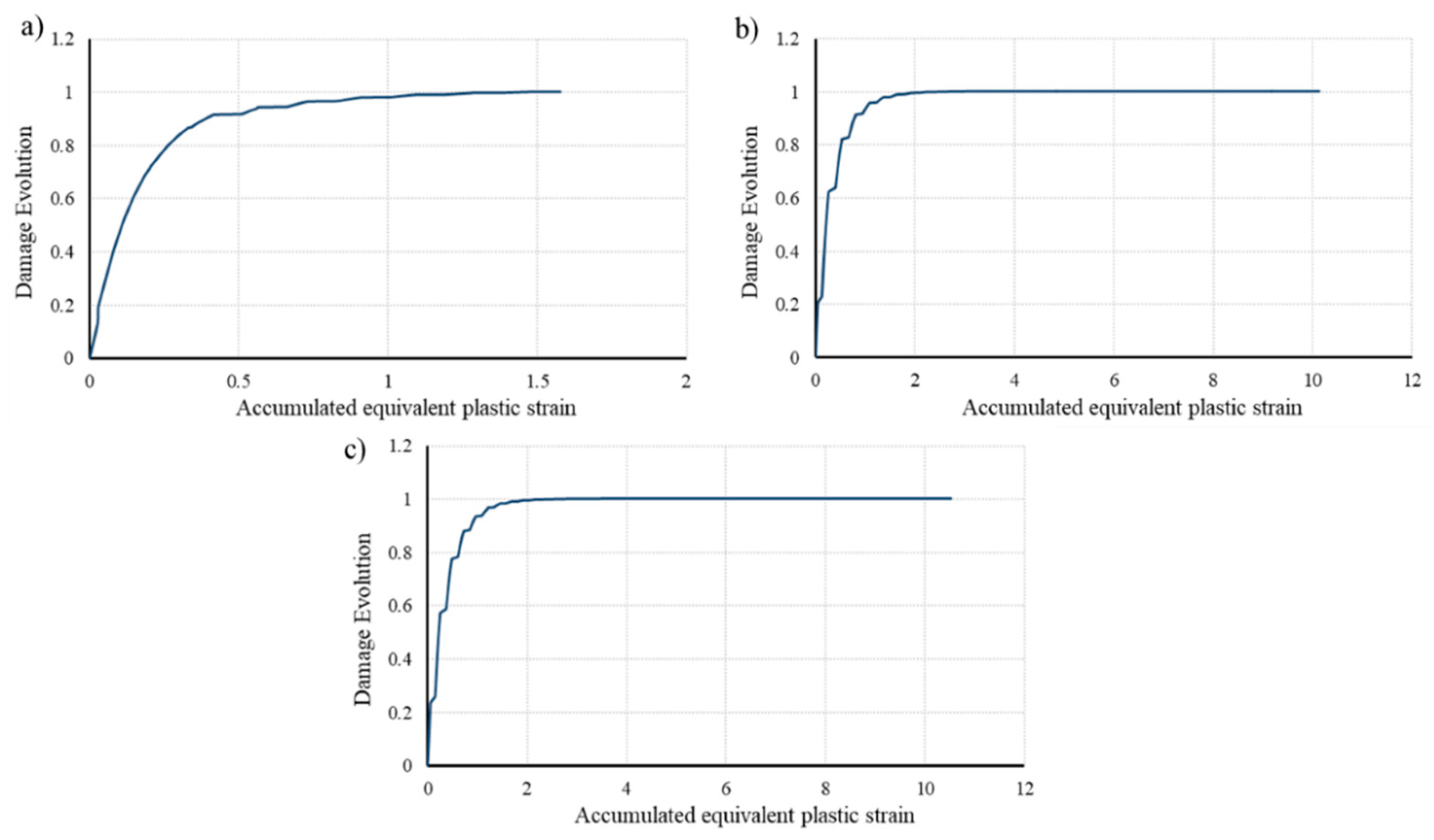
For the three “R2” specimens (Figure 11a–c), the damage evolution was seen to increase in a similar process as in the “R1” specimens. In Figure 11a, the number of high-strain reversed cycles to failure was ten cycles. The number of reverse loading cycles to failure in Figure 11b,c are 41 and 51 cycles, respectively. The damage accumulation for the specimens in Figure 11b,c rapidly increase in the first couple of cycles then decrease to a point where the increment becomes approximately 0.01 in the final counts of cycles. Lastly, the three PE specimens (Figure 12a–c) depict a similar damage accumulation behavior of R2 specimens. The number of reverse loading cycles to failure in Figure 12a–c are 10, 21, and 43 cycles, respectively.

In summary, the damage evolution is shown to behave nonlinearly. This result verifies that the damage evolution in ELCF is very high in the first reverse cycles and decreases as the cycling loading continues until failure. Thus, the damage evolution rate during ELCF is nonlinear. Accordingly, we expect an excessive deterioration in the material’s microstructure during the early cycles of ELCF and less deterioration in the remaining cycles until failure. In between the early number of cycles and the crack initiation, a transition phase in the damage evolution is seen in the damage curve, where the evolution changes from high and rapid to low and slow. 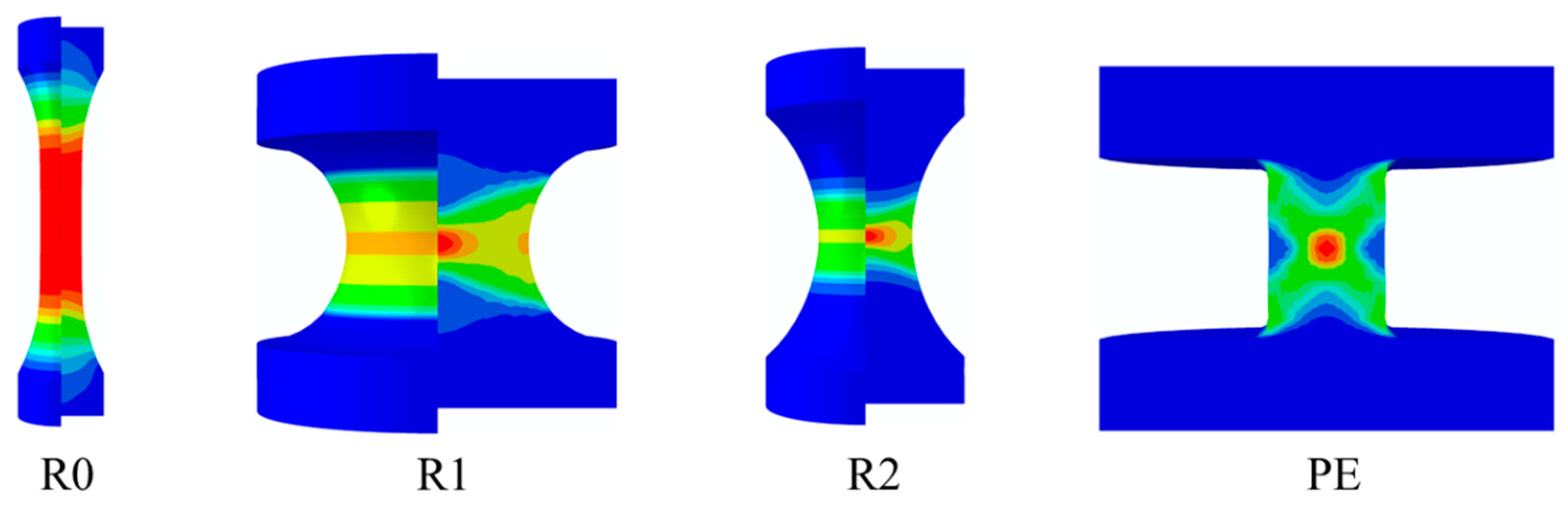Figure 13 shows the specimens’ deformation in FEA during the cyclic loading and the damage accumulation within the specimen’ center. The highest damage accumulation (in red) during ELCF is where the voids coalesce and therefore a crack initiate.

5.2. Fatigue Crack Initiation and Propagation

Studying fatigue, over the years, essentially involves analyzing the loss of a metal’s strength and predicting a metal’s life. This approach is essential in studying metal fatigue to help comprehend the crack initiation and propagation that occurs during the cyclic loading process. In high-cycle fatigue (HCF) (N_f > 10⁴) and low-cycle fatigue (LCF) (10⁴ > N_f > 10²) regimes, cracks initiate and progressively propagate until failure. In these two regimes, the fatigue crack mechanism starts once a metal’s microstructure deforms due to repetitive application of stress. After that, microcracks initiate at the surface and then coalesce to form larger cracks. The final metal failure occurs as the cracks propagate inwards [38].

On the other hand, the phenomena of crack initiation and propagation (aforementioned) for HCF and LCF does not uniquely take a role in the ELCF regime. Researchers claim that the ductile fracture failure mechanism is part of the ELCF failure as well as the fatigue failure mechanism. However, the ductile fracture mechanism takes the principal and major role in ELCF failure [39].

Experimental observation reveals strong resemblances between the fracture surfaces due to ELCF and the ductile fracture. Studies presumed this resemblance as a result of the high strain amplitudes applied that lead to significant ductility exhaustion within the metal. Moreover, fracture surfaces due to ELCF show no signs of beach marks (clamshell marks). Nevertheless, fracture surfaces as a result of ELCF display a cup-cone fracture mode for the axisymmetric specimens “R2” and “R1” and slant fracture mode for the plane-strain specimens “PE” (Figure 14), similar to fractured specimens due to ductile fracture in [23]. This observation supports the notion that cracks due to ELCF tend to initiate in the gauge center of the specimen and propagate outwards towards the surface. In Figure 15, Figure 16 and Figure 17, SEM pictures of the fracture surface profile show microvoids growth and coalescence due to the very high plastic strain during ELCF for “R1”, “R2”, and “PE” specimens. In the same vein, no signs of striations nor fatigue–fracture transition on the fracture surfaces are observed under high magnification.

6. Conclusions

Predicting and evaluating the damage evolution caused by ELCF with mathematical models is crucial and challenging. An extended damage accumulation model for ELCF life prediction was developed with the aid of experimental data in Reference [1]. Four distinctive geometries were designed to study the effect of different stress states on ELCF life and damage evolution. The four specimen’s geometries were designed in such a way to attain different stress states, three of which are classified as axisymmetric stress states and one is classified as a plane-strain stress state. Investigating multiaxial damage evolution due to ELCF can be performed by inspecting three distinguished features on the specimen’s fracture surface: the crack initiation site, the crack growth surface area, and the final fractured surface. The irreversible damage mechanism is quantitatively represented by the accumulated damage $\mathrm{D}$ in Equations (6) and (7). The damage model is calibrated for life prediction to agree with the ELCF experimental results. After that, the damage evolution is extracted from Abaqus and plotted versus the accumulated ${\overline{\mathsf{\epsilon }}}_{\mathrm{pl}}$. The results are as follows:

• The results of the damage evolution plot show that the ELCF damage behaves in a nonlinear manner.
• The ELCF damage evolution for all stress states (Figure 10, Figure 11 and Figure 12) was seen to increase rapidly in the first couple of cycles until the accumulated equivalent plastic strain reaches a certain value then it starts to accumulate slowly as the cycling process continues. This slow evolution in damage becomes even slower as the specimen reaches its life limit (D = 1).
• There is excessive deterioration in the metal microstructure during the early cycles and less deterioration in the remaining cycles until failure.
• In all stress states, the damage evolution during compression loading is very small (≈0.0001) and almost negligible.
• This FEA simulation of the damage accumulation models the crack initiation location in the specimens’ center similar to what have been seen in the experimental results.
• The fracture surface shows that the ductile fracture failure mechanism is part of the ELCF failure as well as the fatigue failure mechanism. Moreover, it is observed that the ductile fracture mechanism takes the dominant role in very high strain cyclic loading.
• SEM pictures demonstrate microvoids nucleation, growth, and coalescence, with no signs of striations due to ELCF.

Finally, it is recommended for future-related research to increase the number of test specimens to replicate the test results in order to study the variability associated with the observations and conclusions. It is also recommended to use transmission electron microscopy (TEM) to perform extra examinations for the fractured surfaces to add additional insight into the dislocation configurations in ELCF specimens. In addition, in situ X-ray tomography during the cycling loading tests can further assist in monitoring and observing the fracture mode and failure mechanism [40,41,42].