Neural Network Modeling for the Extraction of Rare Earth Elements from Eudialyte Concentrate by Dry Digestion and Leaching

Abstract

Eudialyte is a promising mineral for rare earth elements (REE) extraction due to its good solubility in acid, low radioactive, and relatively high content of REE. In this paper, a two stage hydrometallurgical treatment of eudialyte concentrate was studied: dry digestion with hydrochloric acid and leaching with water. The hydrochloric acid for dry digestion to eudialyte concentrate ratio, mass of water for leaching to mass of eudialyte concentrate ratio, leaching temperature and leaching time as the predictor variables, and the total rare earth elements (TREE) extraction efficiency as the response were considered. After experimental work in laboratory conditions, according to design of experiment theory (DoE), the modeling process was performed using Multiple Linear Regression (MLR), Stepwise Regression (SWR), and Artificial Neural Network (ANN). The ANN model of REE extraction was adopted. Additional tests showed that values predicted by the neural network model were in very good agreement with the experimental results. Finally, the experiments were performed on a scaled up system under optimal conditions that were predicted by the adopted ANN model. Results at the scale-up plant confirmed the results that were obtained in the laboratory.

1. Introduction

Rare earth elements (REE) consist of scandium, yttrium, and the group of 15 lanthanide elements, which are characterized by similar chemical properties and commonly occur in the same deposits [1]. Currently, REE are vital component of many modern technologies, including electric and conventional cars, computers and smart phones, renewable energy infrastructure, and phosphor light [2,3,4]. Their unique properties, such as radiation emission or magnetism, allow for REEs to be used in many different therapeutic and diagnostic applications in modern medicine.

Due to the enormous significance that REEs will have in the future, research that is related to REEs is essential in many aspects: mineralogy, location of the world’s REE deposits, classic and alternative extraction technologies, etc. Concerning mineralogy, the conventional primary minerals involve bastnaesite, monazite, xenotime, REE phosphate minerals, and ion adsorption minerals. The authors in [5] are focused on REE Mineralogy and Resources, which might be used for the recovery of Heavy rare earth elements concerning to the future green technologies. Bayan Obo in China and Mountain Pass in USA possess the largest carbonatite deposits around the world, which show light REE enrichment. Ion-adsorption REE ore deposits that are mainly distributed in southern China, and the grade of heavy REE is high in it. Other ore deposits tend to be distributed unevenly globally [6,7]. Nowadays, above 90% of the REE in the world market is supplied by China, which has abundant rare earth mines. Demand for REE has been constantly increasing in last decades and is expected to grow even stronger in the future [8,9]. As such, many projects have been initiated all over the world, which seek to find alternative sources of REE outside China [10,11,12]. Except the secondary resources, a variety of potential unconventional deposits have also been explored, such as REE-bearing laterite, peralkaline granite, ferromanganese nodules, and silicate deposits, including eudialyte, mosandrite, and britholite [13,14,15,16]. Among the minerals mentioned, Eudialyte is a promising REE resource, which contains 1.5–2% REE [17]. Eudialyte is a somewhat complicated cyclosilicate mineral, which forms in alkaline igneous rocks, such as nepheline syenites. It tends to be rich in zirconium, beryllium, cerium, niobium, barium, yttrium, and other rare earth elements [18,19]. The typical chemical formula of Eudialyte is Na₄(Ca, Ce, Fe)₂ZrSi₆O₁₇(OH, Cl)₂, but the component of the mineral may be sometimes different because of the zeolite crystal structure, which possesses ion-exchange properties of eudialyte [20,21].

The technologies for the REE recovery vary depending upon the characteristics of initial material. Using acid, alkali, or chemical salts to decompose and extract represent the common ones. For example, REE in ion-adsorption ore can be readily extracted with ammonia sulfate solution. To extract REE from eudialyte, technological strategies, like decomposition with sulfuric, hydrochloric, and nitric acids have already been suggested and partly researched in the laboratory. Despite being easily decomposed with acids, the treatment can be very challenging as co-dissolved silica forms a gelatinous mass of the whole suspension [22,23,24]. Russian teams [22,23] studied the hydrometallurgical treatment of eudialyte in an earlier period, and the advisable technology would be a two stage decomposition process by sulfuric acid. Sodium sulfate solution was used to dilute the slurry after the first decomposition by acid, keeping REE staying in the solid as double sulfate salts. REE were recovered in the subsequent stage, washing and converting the sulfates into nitrates or chlorides. However, it required much excess acid to avoid the formation of silica gel [22,25]. Another choice is reaction with hydrogen fluoride [23]. It was pointed out fluoride ion can facilitate the decomposition of eudialyte as well as prevent gel formation. The major drawback of this process is safety concern as HF is used. After using a beneficiation process (a combination of gravity and magnetic separation), the authors of [26] studied hydrometallurgical processing of eudialyte Norra Kärr (Sweden) through various leaching experiments with sulfuric acid. In this project, dry digestion with HCl was not applied. Rivera et al. have studied the extraction of rare earth elements from bauxite residue (red mud) by dry digestion followed by water leaching through multi-stage circulation of acid in small laboratory scale [27], but mathematical modeling and process optimization was not performed.

According to the latest research [17], fuming (“Dry digestion at temperatures about 100 °C”), the addition of an acidic solution to heated eudialyte concentrate, and the subsequent water leaching of the treated concentrate could result to the high recovery of REE with avoiding silica gel formation. Moreover, in the mentioned paper, Davris et al. studied hydrometallurgical processing of eudialyte bearing concentrates, using high concentrated acid to recover rare earth elements via low-temperature dry digestion to prevent silica gel formation. Both fuming and low-temperature dry digestion processes confirmed HCl performs higher recovery of REE when compared with H₂SO₄. It was found that dry digestion with high concentrated HCl benefits the extraction of REE and prevents gel formation. The recommended concentration of HCl to decompose the eudialyte concentrate is 10 mol/L [24].

In this paper, the dry digestion process was studied without external heating. In order to reduce the number of complex laboratory experiments, the design of experiments theory (DOE) was firstly used in order to create an optimal central composite design plan (CCD). This approach for the extraction of rare earth elements is missing in literature, and is not present in the previous work of Voßenkaul [24]. In addition, information on upscaling operations for the treatment of eudialyte is missing in overall literature. In order to obtain the optimal regime for the REE extraction process, based on the realized DOE plan, we performed modeling of this process via Multiple Linear Regression (MLR), Stepwise Regression (SWR), and Artificial Neural Network (ANN). To our knowledge, no previous work has been reported on ANN modeling for the extraction of rare earth elements from eudialyte concentrate by dry digestion and leaching. Our goal was to verify the feasibility of low temperature acid treatment of eudialyte concentrate on a scale-up demonstration plant using the obtained optimal set of process parameters.

2. Theoretical Background

Theoretical background of applied methods—MLR, SWR, DOE, and ANN—is shown in the following subsections.

2.1. Multiple Linear Regression

MLR is used to model the linear relationship between a response variable and one or more predictor variables. MLR model represents a linear combination of regression coefficients ${\beta }_i$ and regressors, in the form of $\mathbf{X}=f_i({\mathbf{x}}^{\mathbf{T}})$, named basis functions or states: $\eta =\eta (\mathsf{\beta },\mathbf{x})={\displaystyle \sum _{i=0}^d{\beta }_i·}{f}_i({\mathbf{x}}^{\mathbf{T}})$. Vector $\mathbf{x}$ is a vector of predictors, $\mathsf{\beta }$ is a vector of regression coefficients, and $d$ is the number of basis functions. In MLR, the unknown coefficients ${\beta }_i(i=0,d)$ are estimated by values $b_i(i=0,d)$, which were obtained by using experimental results. In matrix notation, the least squares estimator of $\mathsf{\beta }$ is $b={(X^T·X)}^{-1}·X^T·\mathbf{Y}$. Vector $Y$ is a vector of output variables, the fitted model is given by $\widehat{Y}=\mathbf{X}·\mathbf{b}$, and the vector of the residuals is $\mathsf{\epsilon }=\mathbf{Y}-\widehat{Y}$ [28,29,30].

2.2. Stepwise Regression

Stepwise regression is essentially based on semi-partial correlation, which is expressed through the semi-partial correlation coefficient ($sr$) and the square of this coefficient ($s{r}^2$). The square of the semi-partial correlation coefficient, for a specific single variable, indicates by how much the $R^2$ value will reduce if this single variable is removed from the regression equation. $R^2$ denotes the coefficient of multiple determination.

Let $\chi$ be the set of all the independent variables $X$, and ${\psi }_k$ be the set of all the independent variables $X$ except for $x_k$. Then, the squared semi-partial correlation coefficient is expressed as follows in (1):

$$s{r}_k^2=R_{\chi }^2-R_{{\psi }_k}^2$$

(1)

Form of expressing semi-partial correlation coefficients may vary, and one of the most common forms is (2):

$$s{r}_k=\frac{t_k·\sqrt{1-R_{\chi }^2}}{\sqrt{residualDF}}$$

(2)

where $t_k$ is the Student’s t-statistic value for the $k$th regressor in the MLR model, $residualDF=N-K-1$, denotes the number of degrees of freedom for the sum of residuals, $N$ is number of measurements, and $K$ is the number of regressors. Stepwise regression is explained in detail in [28,30,31].

2.3. Design of Experiments

Design of experiment (DOE) was performed in order to decrease the number of necessary experiments, required time, and operational costs. This method stems from the studies of Fisher [32] and Box and Wilson [33]. With DOE, the research hyperspace can be explored with high efficiency, factor interactions can be revealed, and a substantial volume of response space can be covered. In this paradigm, D-optimality criterion is the basis for the design matrix, as denoted by $X$, which contains a set of experimental points, which lie on the border of the hyper sphere, forming a hypercube [28]. In order to make this analysis simple, the process variables associated with factors $X_i$ are encoded using the following equations,

$$x_i=\frac{X_i-X_{0i}}{w_i},(i=1,2,3\dots ,k)$$

(3)

$$X_{0i}=\frac{X_{i\max }+X_{i\min }}{2},w_i=\frac{X_{\max }-X_{\min }}{2·\alpha }$$

(4)

where $k$ denotes the number of significant factors, $X_i$ is an actual value of the $i$th factor, $X_0$ represents the arithmetic mean for factor $X_i$ (basic level), and $w_i$ is the interval of its variation. The actual value of alpha depends of the number of factors: $alpha=2^{k/4}$ and has a value of 1.41 for two factors, 1.682 for three factors, etc. For example, an experimental plan with three factors ($k=3$) for first order MLR, in schematic form is given in Figure 1a. In the encoded domain, the highest factor level corresponds to +1, the lowest level to −1, and the basic level to 0. The grey point in the center of the cube is the center point of the experiment design. It is usually expected that the performed experiments shall be repeated in the central point in order to determine the experimental error [28].

Polynomial regression models in the second-order MLR form require additional experimental points. For full factorial orthogonal rotatable central composite design (CCD), additional experimental axial points are at the distance alpha from the central point. Schematic view of design of experiments for this kind of model is shown in Figure 1b.

CCD factorial design is a common approach for research optimization with a limited number of experiments [34]. MLR models of higher order require additional measurements. However, additional experiments would increase the investigation costs.

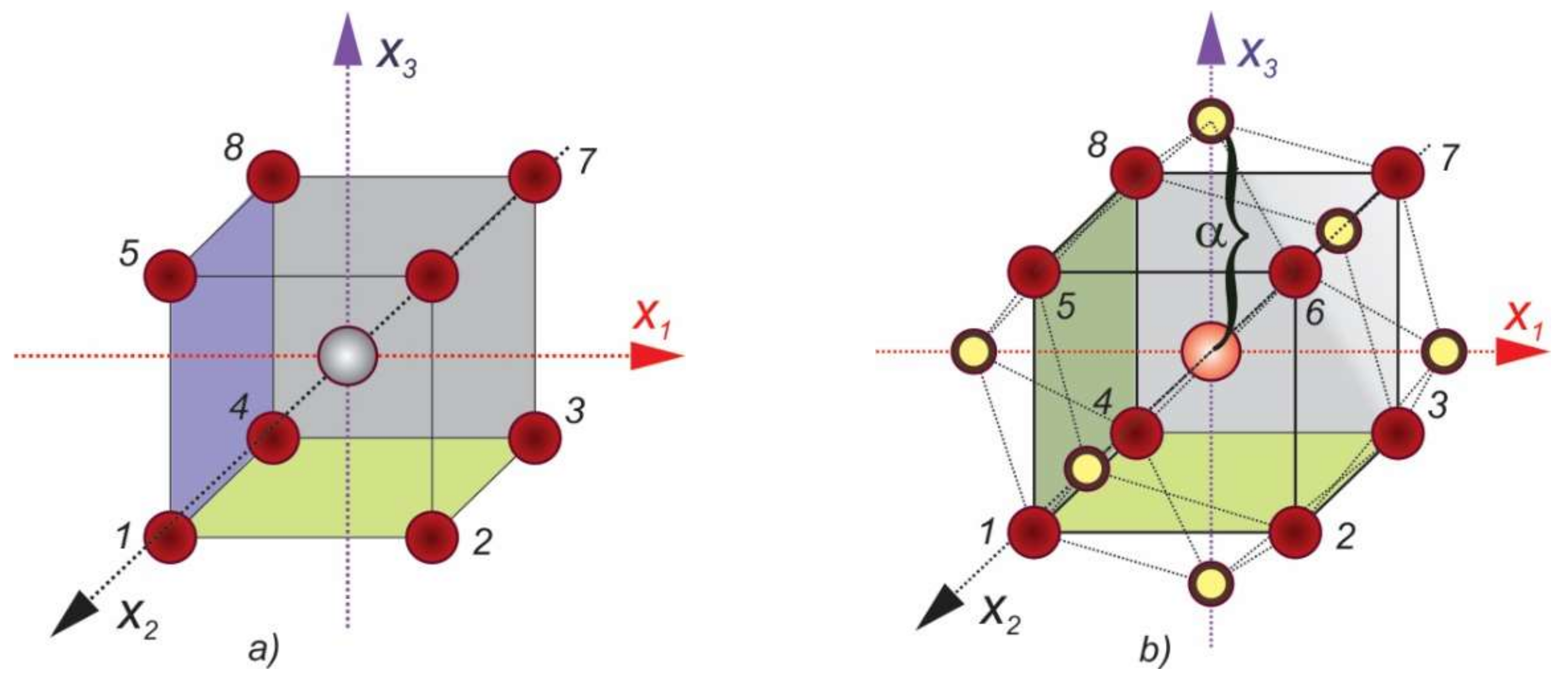
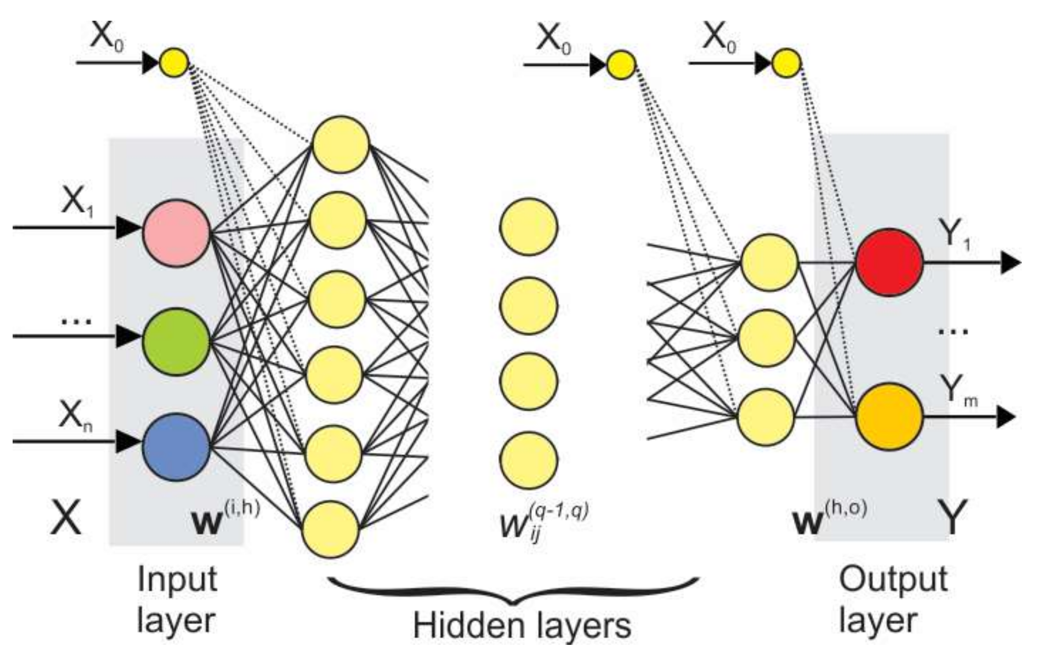
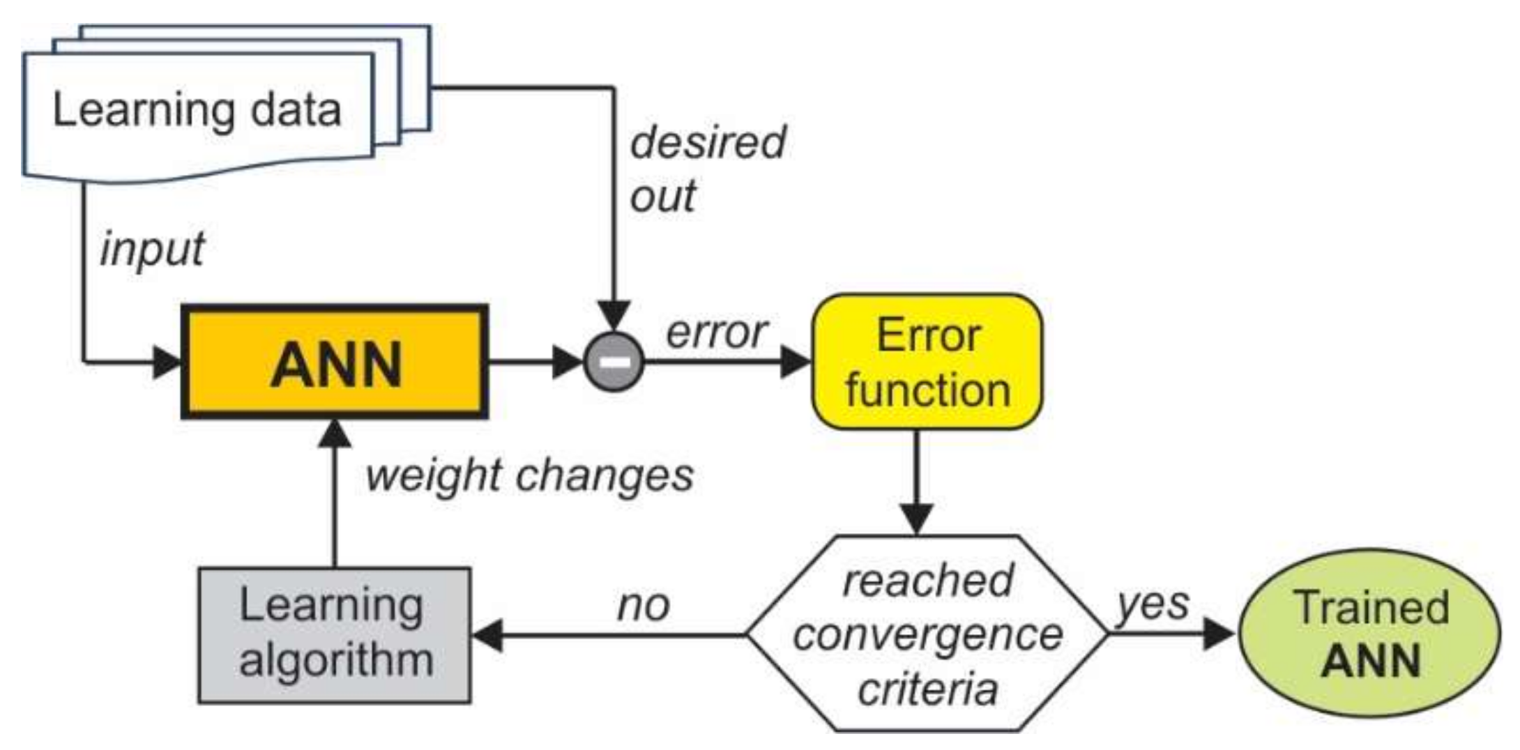
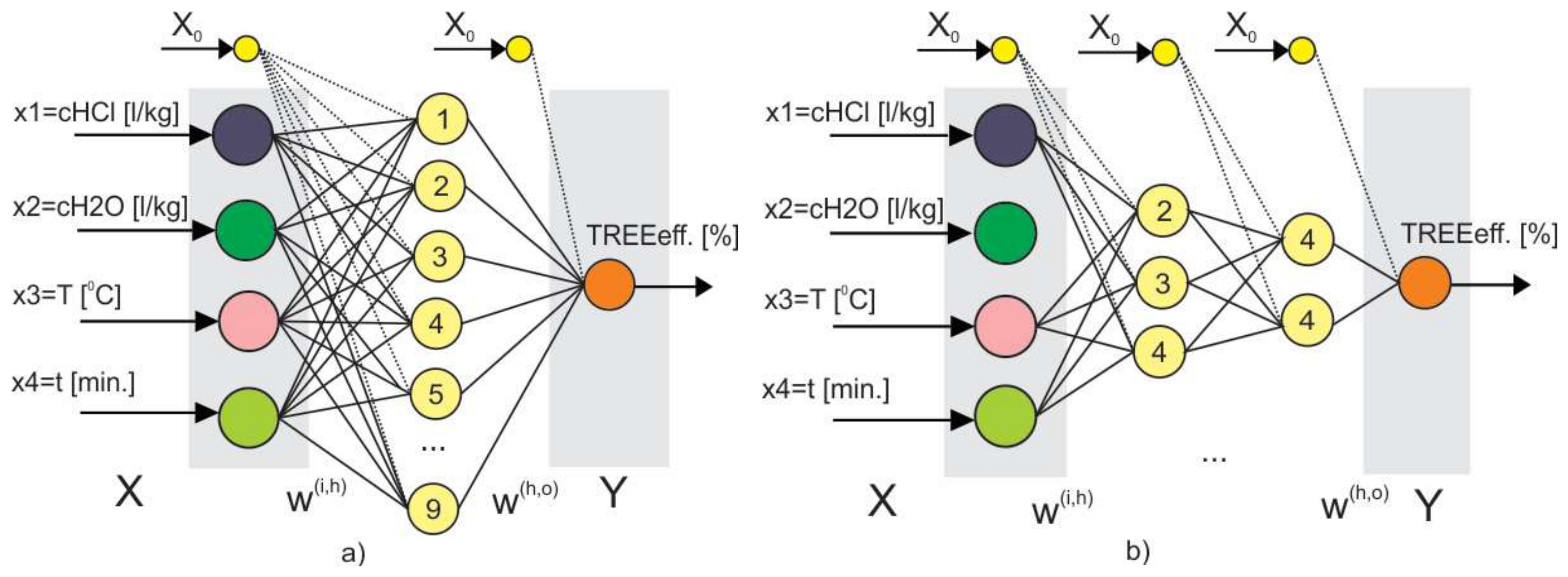
2.4. Artificial Neural Network

Among many different types of ANN, the feed-forward ANN is the most widely researched and used [35,36,37]. A feed-forward network has many layers. The structure of a feed-forward ANN is given in Figure 2.

In Figure 2 $X$ denotes the vector of input variables, $Y$ is the vector of output variables, $w^{(\mathbf{i},\mathbf{h})}$ is a column-matrix of weight coefficients between neurons in the input layer and the first hidden layer, and $w^{(\mathbf{h},\mathbf{o})}$ is a column-matrix of weight coefficients between the neurons in the last hidden layer and the output layer. The term $w_{ij}^{(q-1,q)}$ denotes the weight between $i$th neuron from $(q-1)$th hidden layer and $j$th neuron from ($q$)th hidden layer.

The total input ${\alpha }_j^{(q)}$ into processing element $j$ in $q$th layer is a weighted sum of all the outputs $x_i^{(q-1)}$ from the previous layer. The activation function, $x_j^{(q)}=AF({\alpha }_j^{(q)})$, transforms the input signal, ${\alpha }_j^{(q)}$, to the output signal—$x_j^{(q)}$. Most frequently used activation functions are: logistic sigmoid, hyperbolic tangent, and rectified linear unit.

Values of all the ANN weight coefficients are determined using a learning process. The goal is to minimize the error function (difference between desired and predicted values). One of the most popular ANN learning algorithms is the backpropagation algorithm. According to this algorithm, the error is propagated backward through the network and the weights are updated through a number of iterations (Figure 3). The procedure progresses until it reaches convergence or a given maximum number of iterations [38].

In this work we used some commonly used variations of the backpropagation algorithm: The Backpropagation gradient descent algorithm (BPGD) [39,40], the Resilient backpropagation algorithm (RPROP) [41,42], and adaptive moment estimation algorithm (ADAM) [43].

Design of a neural network is determined by various ANN hyperparameters: number of hidden layers, number of neurons in each hidden layer, number of training samples, initial set of weights, the range of initial weights, etc. Some recommendations for hyperparameter choice are given in [44].

3. Materials and Methods

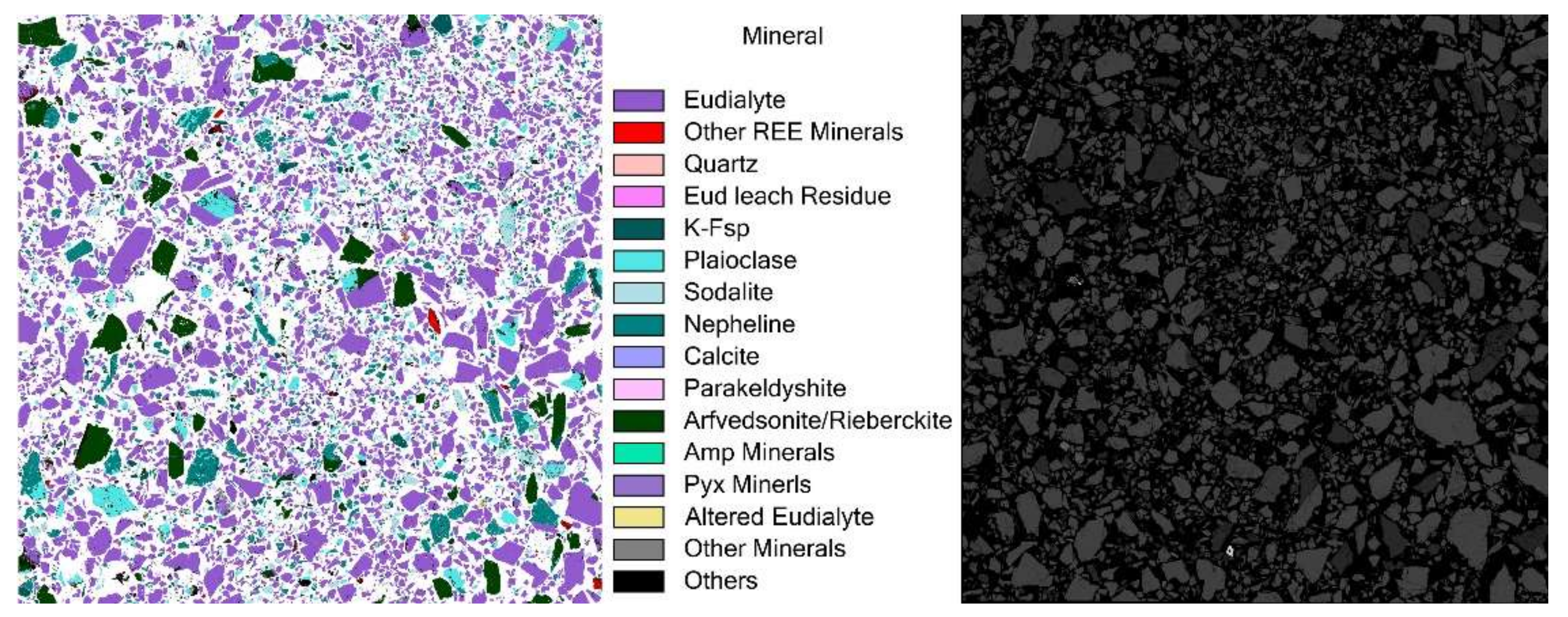
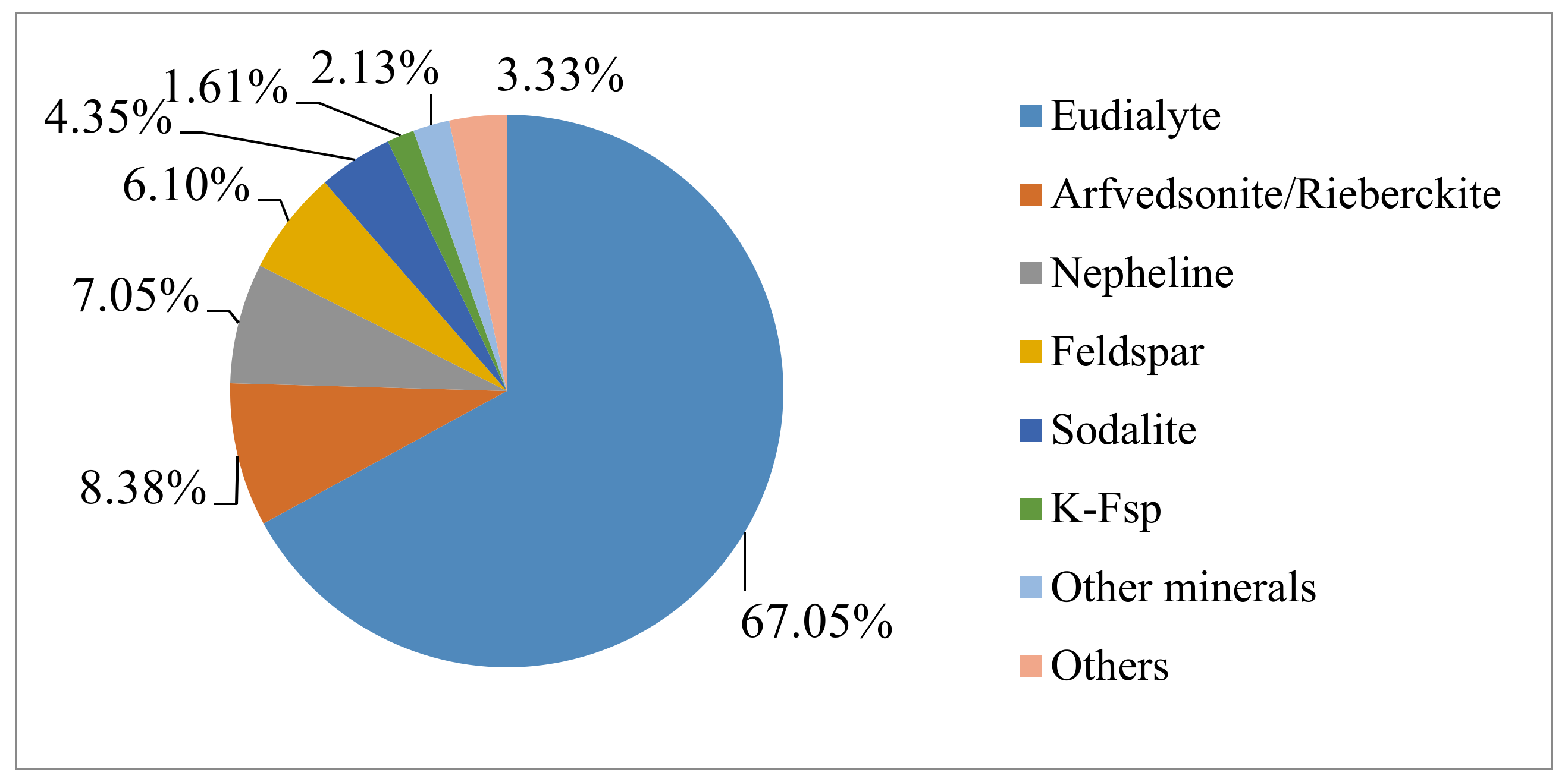
3.1. Material and Analysis

Eudialyte concentrate from Tanbreez ore exploited in southern Greenland was used as raw material. The name Tanbreez is the acronym of Ta, Nb, REE, and Zr. The chemical composition of the eudialyte concentrate supplied by Geological Survey of Finland (GTK) is given in

Table 1. Chemical composition of eudialyte concentrate by XRF (X-ray fluorescence).

Element	Content (wt %)	Element	Content (wt %)
Al	3.2	Ce	0.52
Ca	5.7	Pr	532 mg/kg
Fe	6.04	Nd	0.21
Mn	0.39	Sm	440 mg/kg
Nb	0.36	Gd	239 mg/kg
Zr	5.08	Dy	580 mg/kg
Hf	0.11	Y	0.33
Si	23.1	Yb	368 mg/kg
La	0.25	TREE	1.52

. The composition of eudialyte concentrate and solid residue were analyzed by X-ray fluorescence (AXIOS, PANanalytical, Eindhoven, The Netherland) and the elements in the solution were analyzed by ICP-OES (SPECTRO ARCOS, SPECTRO Analytical Instruments GmbH, Kleve, Germany). The QEMSCAN results in Figure 4 reveal the mineral distribution of eudialyte concentrate by false red color image and the right is the BSE image. The mineral composition and the microstructure were determined by QEMSCAN (Quantitative Evaluation of Materials by SCANning electron microscopy), (FEI/Thermo corporate headquarters, North America Nanoport, Hillsboro, OR, USA). The phase quantification is summarized in Figure 5. Eudialyte accounts for 67.05% in the eudialyte concentrate and the concentrate contains some other silicate minerals, such as Arfvedsonite, Nepheline, and Feldspar.

Commercial grade HCl (31%) with molarity of 10 mol/L and tap water without further purification were used, both in the laboratory and scale-up plant.

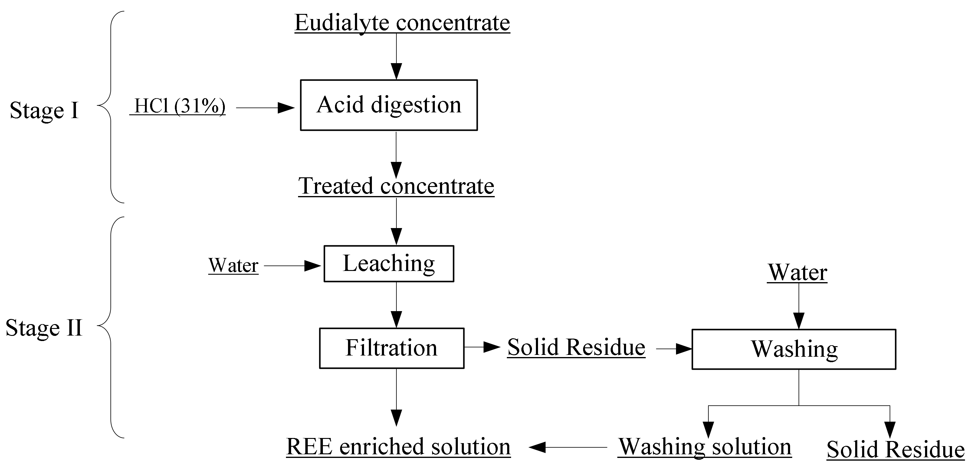
3.2. Extraction Procedure

The operation flowchart is shown in Figure 6. Dry digestion process with high concentrated 31% hydrochloric acid represented the first step. The molarity of the used acid was 10 mol/L. Taking advantages of the exothermic reaction, the temperature could reach about 80 °C without external heating. The aim was to decompose eudialyte concentrate and form metal chloride salts without silica gel formation by forming silica precipitation. The specified amount of water was subsequently added to the sludge after digestion, achieving REE leaching and allowing low silica to be dissolved into the leaching solution. Therefore, the maximum REE extraction process time (dry digestion and leaching) in the laboratory was 2 h. After filtration and washing the filter cake, a REE enriched solution and solid residue were obtained.

4. Experiments and Obtained Measurements of Process Outputs

During research we chose to investigate four factors ($k=4$), namely hydrochloric acid to the concentrate ratio ($c\mathrm{HCl}$), water to the concentrate ratio ($c{\mathrm{H}}_2\mathrm{O}$), leaching temperature ($T$), and leaching time ($t$). The chosen parameters were proposed concerning the previous experimental work at the EURARE Project [11], literature data [17,24], and high experience of the authors in hydrometallurgy.

The arrangement of experimental points for $k\ge 4$ cannot be visualized, but it is easily described using a design matrix. In accordance with CCD plan, the central point experiments were repeated seven times to guarantee a more precise determination of an experimental error. Eudialyte concentrate mass in all laboratory experiments was 500 g. The total experimental design matrix and the obtained results are given in

Table 2. Experiment design matrix.

No.	X1:HCl:Con. (L:kg)		X2:Water:Con. (L:kg)		X3:Leaching Temp. (°C)		X4:Leaching Time (min.)		Y:TREE Extr. (%)
	1:1, 1.25:1, 1.5:1		1:1, 2:1, 3:1		20, 50, 80		20, 40, 60		[0–100]
	c.v.	a.v.	c.v.	a.v.	c.v.	a.v.	c.v.	a.v.
A1	1	1.5:1	1	3:1	1	20	1	60	93.475
A2	−1	1:1	1	3:1	1	20	1	60	79.640
A3	1	1.5:1	−1	1:1	1	20	1	60	82.010
A4	−1	1:1	−1	1:1	1	20	1	60	73.940
A5	1	1.5:1	1	3:1	−1	20	1	60	86.465
A6	−1	1:1	1	3:1	−1	20	1	60	79.070
A7	1	1.5:1	−1	1:1	−1	20	1	60	81.170
A8	−1	1:1	−1	1:1	−1	20	1	60	79.450
A9	1	1.5:1	1	3:1	1	20	−1	20	85.350
A10	−1	1:1	1	3:1	1	20	−1	20	80.630
A11	1	1.5:1	−1	1:1	1	20	−1	20	76.940
A12	−1	1:1	−1	1:1	1	20	−1	20	71.140
A13	1	1.5:1	1	3:1	−1	20	−1	20	77.650
A14	−1	1:1	1	3:1	−1	20	−1	20	75.525
A15	1	1.5:1	−1	1:1	−1	20	−1	20	88.600
A16	−1	1:1	−1	1:1	−1	20	−1	20	80.090
A17 *	0	1.25:1	0	2:1	0	50	1	40	89.49, 87.99, 88.74, 90.85, 86.63, 94.35, 83.24

Note: c.v., coded value; a.v., actual value; * repeated experiments in the central point.

.

The average total rare earth elements (TREE) extraction efficiency of all the experiments was over 80%, and the mean value of the central point A17 was 88.756% with a standard deviation of 3.458%.

Correlation analysis offers the following values of the Pearson between predictor variables: $c\mathrm{HCl}$, $c{\mathrm{H}}_2\mathrm{O}$, $T$ and $t$ at one side, and a dependent variable ${\mathrm{TREE}}_{\mathrm{eff}.}$—TREE extraction efficiency, on the other side: $r_{{\mathrm{TREE}}_{\mathrm{eff}.}-c\mathrm{HCl}}=0.5631$, $r_{{\mathrm{TREE}}_{\mathrm{eff}.}-c{\mathrm{H}}_2\mathrm{O}}=0.2640$, $r_{{\mathrm{TREE}}_{\mathrm{eff}.}-T}=-0.0528$ and $r_{{\mathrm{TREE}}_{\mathrm{eff}.}-t}=-0.2082$, respectively. According to advice in [45], the variables should be considered in a regression model only for $r>0.3$. However, in order to perform a detailed analysis, the relationship of the leaching temperature and total rare earth elements extraction efficiency is also studied.

5. Model Setup and Results

5.1. Process Modeling in MLR Form

In this paper, we used the following MLR models:

(a)

first order multiple linear regression

$$y=b_0+{\displaystyle \sum _{i=1}^k{b}_i}·x_i$$

(5)

(b)

first order multiple linear regression with interaction effects

$$y=b_0+{\displaystyle \sum _{i=1}^k{b}_i}·x_i+{\displaystyle \sum _{i=1}^{k-1}{\displaystyle \sum _{j=i+1}^k{b}_{ij}}·x_i·x_j+{\displaystyle \sum _{i=1}^{k-2}{\displaystyle \sum _{j=k+1}^{k-1}{\displaystyle \sum _{l=j+1}^k{b}_{ijl}·}{x}_i·x_j·x_k}}}$$

(6)

where $k$ denotes the number of input factors ($k=4$).

The statistical data analysis in this paper was performed in the R programming language [46]. Model adequacy was tested using Fisher’s F-test. Model given by (5) was adequate, according to the F-test. Its regression parameters, together with its 95% confidence intervals are given in

Table 3. Multiple Linear Regression (MLR) models, regression coefficients and their 95% confidence interval, F-test values, as well as the standard deviation of residuals σ_res.

First-Order MLR Model: $\mathit{y}\mathbf{=}{\mathit{\beta }}_{\mathbf{0}}\mathbf{+}{\mathit{\beta }}_{\mathbf{1}}\mathbf{·}{\mathit{x}}_{\mathbf{1}}\mathbf{+}{\mathit{\beta }}_{\mathbf{2}}\mathbf{·}{\mathit{x}}_{\mathbf{2}}\mathbf{+}{\mathit{\beta }}_{\mathbf{3}}\mathbf{·}{\mathit{x}}_{\mathbf{3}}\mathbf{+}{\mathit{\beta }}_{\mathbf{4}}\mathbf{·}{\mathit{x}}_{\mathbf{4}}$
${\beta }_0$	$83.144565$	$[81.378-84.911]$	$F_t(f_R,f_E,\alpha )=F_t(12,6,0.05)=4$ $F_{rLF}=3.90$ $s^2(y)=11.958262;s(y)=3.458072$ ${s^2}_{LF}=46.61679$ $F_{rLF}<F_{t}isadequate$, ${\sigma }_{res}=6.8276488$
${\beta }_1$	$3.2609375$	$[1.143-5.379]$
${\beta }_2$	$1.5290625$	$[-0.589-3.647]$
${\beta }_3$	$-0.3059375$	$[-2.424-1.812]$
${\beta }_4$	$1.2059375$	$[-0.912-3.324]$

.

The analytical form of the adequate model in the space of encoded variables is the following:

$$y=83.144565+3.2609375·x_1+1.5290625·x_2-0.3059375·x_3+1.2059375·x_4$$

(7)

After transforming the predictor variables back into their original value domain, the model takes the form of (8) and its graphic representation, for (a) $T=const.=20°\mathrm{C}$, $t=20\min .$ and (b) $T=const.=20$ °C, $t=60\min .$ is given in Figure 7.

$${\mathrm{TREE}}_{\mathrm{eff}.}=59.9058+13.0437·c\mathrm{HCl}+1.5291·c{\mathrm{H}}_2\mathrm{O}-0.010197·T+0.0602969·t$$

(8)

Model (8) confirms the results of correlation analysis, that the leaching temperature ($T$) is not significant. Its changes throughout the range from 20 °C to 80 °C, cause a decrease of TREE extraction percentage only in a very small range from 0.20 to 0.81%, respectively. Figure 7 shows that the percentage of TREE extraction increases as the concentrations of HCl (variable $c\mathrm{HCl}$) and H₂O (variable $c{\mathrm{H}}_2\mathrm{O}$) rise, and that the maximum values of extraction are around 90%. Furthermore, TREE extraction efficiency increases with the extension of time from 20 min. (Figure 7a), to 60 min. (Figure 7b). Although the model is in the form of a hyperplane (7), i.e., (8), adequate ($F_{rLF}=3.9<F_t=4$), it can be observed that the process is characterized by high levels of noise, which is indicated by the standard error ($s(y)=3.458072$). For this standard error value, it is relatively easy to perform proof of adequacy. In addition to the above, although the model (8) is adequate, its accuracy is very low, as can be seen from the value of its parameters: the coefficient of multiple determination ($R^2=0.433$), the adjusted coefficient of multiple determination ($R_{adj}^2=0.244$), and root mean squared error, which is calculated in total for all of the experiments, is $RMSE=4.668$.

This implies the need to describe the process with additional models of class (6). However, the potential number of such models is over 16,000, so the computational costs for modeling via the brute force method would be too high. For this purpose, the following section uses the SWR paradigm. Second order MLR models are not used, since that would require the expansion of the experimental plan with new experiments, according to CCD strategy.

5.2. Modeling with Stepwise Regression

For modeling, which is based on stepwise regression method, SPSS Statistics v24 software (IBM, Armonk, NY, USA) package was used. The initial set of regressors included variables: $c\mathrm{HCl}$, $c{\mathrm{H}}_2\mathrm{O}$, $T$, $t$, $c\mathrm{HCl}·c{\mathrm{H}}_2\mathrm{O}$, $c\mathrm{HCl}·T$, $c\mathrm{HCl}·t$, $c{\mathrm{H}}_2\mathrm{O}·T$, $c{\mathrm{H}}_2\mathrm{O}·t$, $T·t$, $c\mathrm{HCl}·c{\mathrm{H}}_2\mathrm{O}·T$, $c\mathrm{HCl}·c{\mathrm{H}}_2\mathrm{O}·t$, $c\mathrm{HCl}·T·t$, and $c{\mathrm{H}}_2\mathrm{O}·T·t$. These regressors correspond to linear first order models in the form of Equation (6). Model selection method, Forward selection was used, and the Akaike Information Criterion (AICC) was used as the optimality criterion for entry and removal of regressors into or from the model. In the iterative stepwise procedure, a model (2) from

Table 4. Linear regression models generated by means of stepwise procedure.

Coefficients a
Model		Unstandard. Coeff.		Standard. Coeff.	t	Sig.	95.0% Confidence Interval for B		Correlations			Collinearity Statistics
		B	Std. Error	Beta			Lower Bound	Upper Bound	Zero-Order	Partial	Part	Tolerance	VIF
1	(Constant)	64.866	6.293		10.307	0.000	51.452	78.280
	$c\mathrm{HCl}$	13.044	4.943	0.563	2.639	0.019	2.509	23.579	0.563	0.563	0.563	1.000	1.000
2	(Constant)	64.866	5.651		11.478	0.000	52.746	76.986
	$c\mathrm{HCl}$	10.554	4.587	0.456	2.301	0.037	0.715	20.393	0.563	0.524	0.441	0.936	1.068
	$c\mathrm{HCl}·c{\mathrm{H}}_2\mathrm{O}·t$	0.031	0.015	0.425	2.146	0.050	0.000	0.062	0.540	0.497	0.411	0.936	1.068

^a Dependent Variable: TREE_eff. [%].

with accuracy: $R_{adj}^2=0.413$, $RMSE=4.487$ was selected. When considering model (8), we deemed the alternative model (1) an oversimplification of the TREE extraction process. Model (2) satisfies the condition of non–multicollinearity (Tolerance > 0.1 and VIF < 10, Table 4).

In Table 4, the column Standardized Coefficients Beta shows the influence of the regressors on the dependent variable. Its values represent the coefficients of the regression model, normalized to have zero mean and unit variance. Absolute values of these coefficients describe the influence of individual regressors on the dependent variable ${\mathrm{TREE}}_{\mathrm{eff}}$. From column Sig. it can be seen that both regressors ($c\mathrm{HCl},c\mathrm{HCl}·c{\mathrm{H}}_2\mathrm{O}·t$) give a unique contribution to the model because the corresponding values are less than or equal to 0.05. The magnitudes of individual contributions are expressed through semipartial correlation coefficients, Part, i.e., the squared values of these coefficients (0.441² = 0.194481, 0.411² = 0.168921). This further extends the understanding of the significance of the observed regressors, and the sum of Part usually differs from $R_{adj}^2$ due to existence of joint effects.

The analytical form of the selected model is given by Equation (9) and its visual representation, for $t=const.=60\min .$, is given in Figure 8a:

$${\mathrm{TREE}}_{\mathrm{eff}.}=64.86596+10.55357·c\mathrm{HCl}+0.0312·c\mathrm{HCl}·c{\mathrm{H}}_2\mathrm{O}·t$$

(9)

The final parameters of the model are: AICC = 55.213, and the predictor importances are 0.53 and 0.47 for $c\mathrm{HCl}$ and $c\mathrm{HCl}·c{\mathrm{H}}_2\mathrm{O}·t$, respectively. Plot Predicted By Observed (Figure 8b), shows the predicted (fitted) values for the output variable ${\mathrm{TREE}}_{\mathrm{eff}.}$ [%], on the vertical axis and true values of the output variable on the horizontal axis. For a perfect model fit, points on the plot would lie on the diagonal line at an angle of 45°.

Like the linear model (8), the linear model with “interaction” variables (9) is adequate ($F_t(f_R,f_E,\alpha )=F_t(14,6,0.05)=3.956$, $F_{rLF}=3.17$, $F_{rLF}<F_t\mathrm{is}\mathrm{adeuqate}$, ${\sigma }_{res}=6.1580326$). Model (9) does not contain the $T$ predictor, which confirms previous conclusions that the leaching temperature is not significant. Comparison of models (8) and (9) shows that both models are of similar shape (Figure 7b and Figure 8a), but that the model with interactions (9) is a bit more accurate ($RMS{E}_{(9)}=4.487$, $R_{adj(9)}^2=0.413$, in comparison with $RMS{E}_{(8)}=4.668$, $R_{adj(8)}^2=0.244$).

Linear models (8) and (9) are adequate. However, the relatively low accuracy of the models, the complexity of the REE extraction process as well as the high level of dispersion, which can be observed in Figure 8b, suggest the possibility that the modeled extraction process is non-linear. In this context, the following section considers the application of the ANN paradigm for modeling the given process.

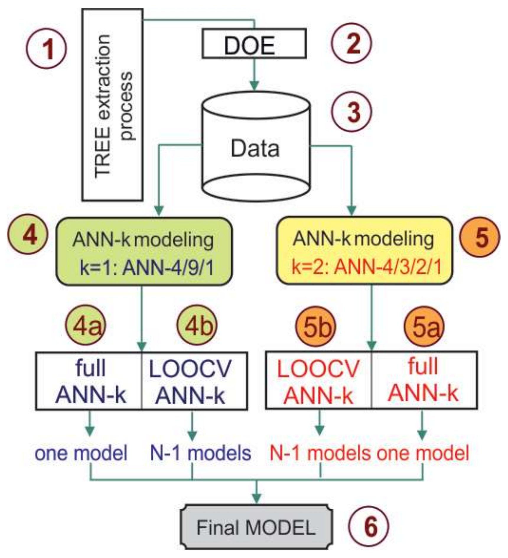
5.3. Modeling with ANN

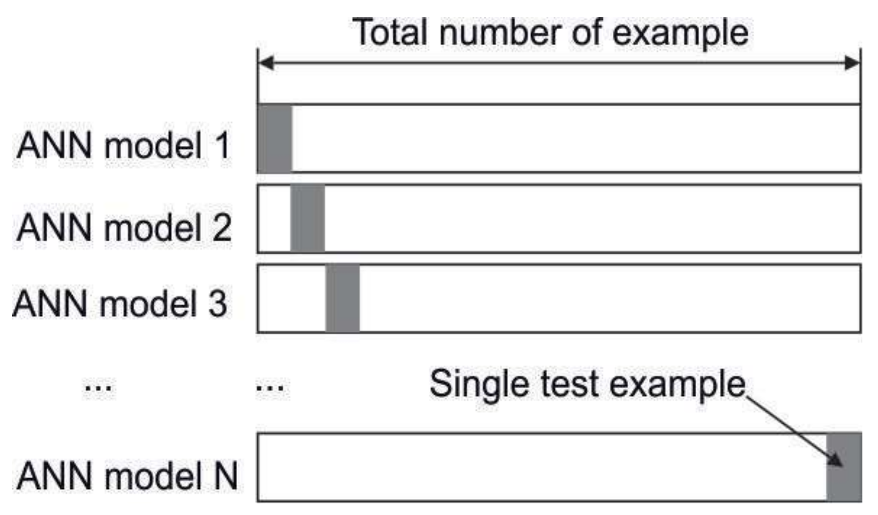
5.3.1. ANN Modeling of TREE Extraction Based on LOO CV

Modeling by artificial neural networks requires a larger amount of data, or a larger number of measurements, than a set of experimental points that were generated by the CCD plan in this study. However, increasing the number of experiments could significantly increase research costs and time. For these reasons, the leave-one-out cross validation (LOO CV) concept, which attempts to generate a stable ANN model from the available data, was applied. This procedure is shown in Figure 9.

Data on the process of TREE extraction (1), based on the realized experiment plan (2), is stored in the database (3). In order to increase stability, modeling is carried out with two network topologies: (4) ANN-4/9/1 with four neurons in the input layer, one output, and nine neurons in the hidden layer, and (5) ANN-4/3/2/1 with four neurons in the input layer, one output, and two hidden layers with three and two neurons. Network architecture (4) is based on the recommendations given in [47], while the network architecture (5) is determined by the trial and error method. Schematic representations of these networks are given in Figure 10a,b.

Each network architecture generates 17 ANN models (N = 17). Models Full ANN_k=1 (4a) and Full ANN_k=2 (5a) were created on the basis of all 17 input/output pairs, where the 17th pair corresponds to the average measurement at the central point of the experimental plan (A17, Table 2). These models represent ANN models, which selected network architectures can generate. In addition, both network architectures (4) and (5) generate 16 ANN models (N − 1 = 16), based on the LOO CV strategy. Leave-one-out Cross validation is a model validation method, which is described in detail in [48]. For very sparse datasets, as in our research, LOO CV can be used in order to train the ANN on the largest possible number of examples. For a dataset with N examples, N ANN models are trained. For each model, N − 1 examples are used for learning (training) and the remaining example for ANN testing (Figure 11).

During each ANN modeling session, we arbitrarily retained in the training set the example that corresponds to the central point of the experiment (A17). In this way, units LOO CV ANN_k=1 (4b) and LOO CV ANN_k=2 (5b) each generated 16 ANN models, as mentioned earlier. Therefore, for ANN LOO CV modeling, only one sample is in the test dataset, but its exclusion from the training dataset significantly influences the ANN model’s form. Due to space, as an example, Figure 12 shows only a few ANN models that were obtained during ANN LOO CV modeling.

The final model (6) on Figure 9, represents a data table numerical model, based on averaging 34 ANN models, which are generated in total by units (4) and (5).

Each $TRE{E}_j$ point of the data table model (6) is calculated according to the Equation (10):

$$TRE{E}_j=\frac{{\displaystyle {\sum }_{k=1}^{2}TRE{E}_{j,i}^{(Full,k)}}+{\displaystyle {\sum }_{i=1}^{N-1}{\displaystyle {\sum }_{k=1}^{2}TRE{E}_{j,i}^{(LOOCV,k)}}}}{2·N}$$

(10)

where $TRE{E}_{j,i}^{(Full,k)}$ denoted $j$th point of $i$th ANN model produced by Full processes (4a) and (5a), while $TRE{E}_{j,i}^{(LOOCV,k)}$ denoted $j$th point of $i$th ANN model produced by LOOCV iterative processes (4b) and (5b). In Equation (10), $k$ denoted net topology: $k=1$ and $k=2$ for ANN-4/9/1 and ANN-4/3/2/1, respectively.

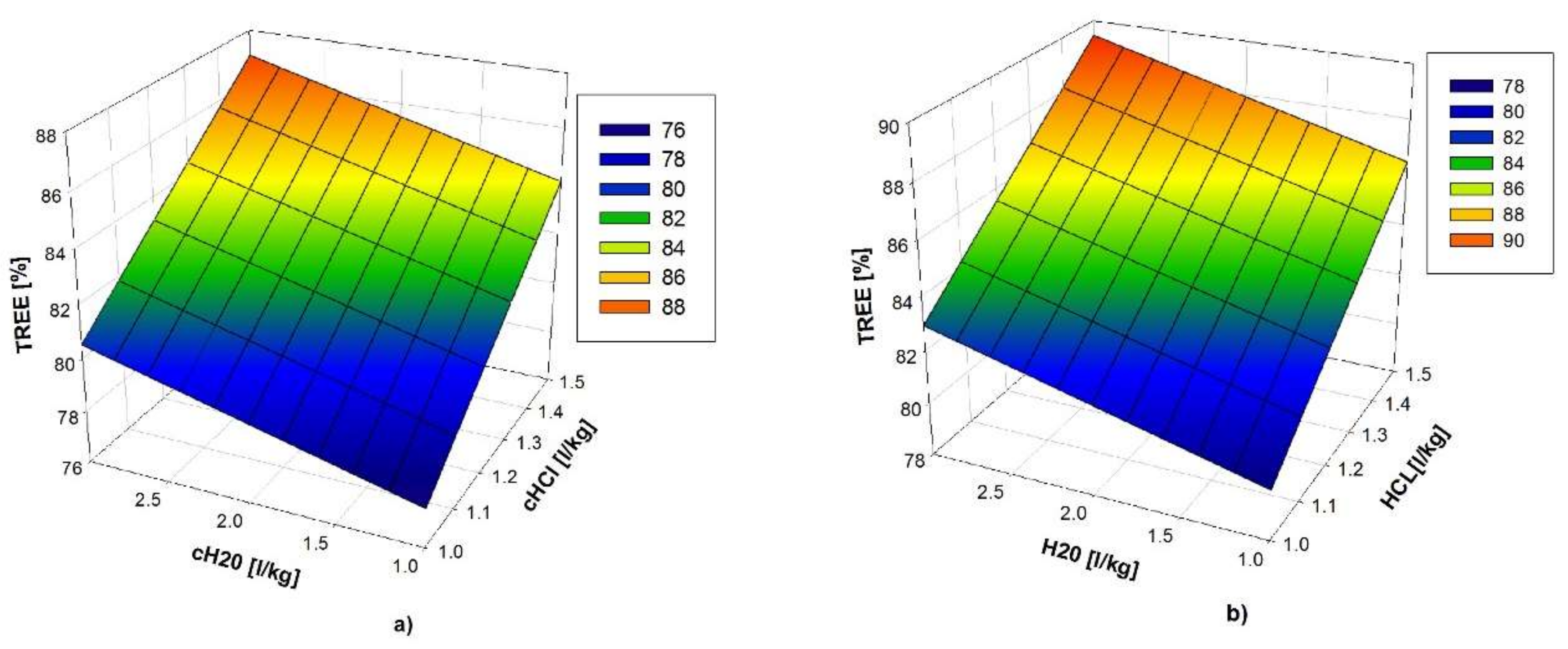
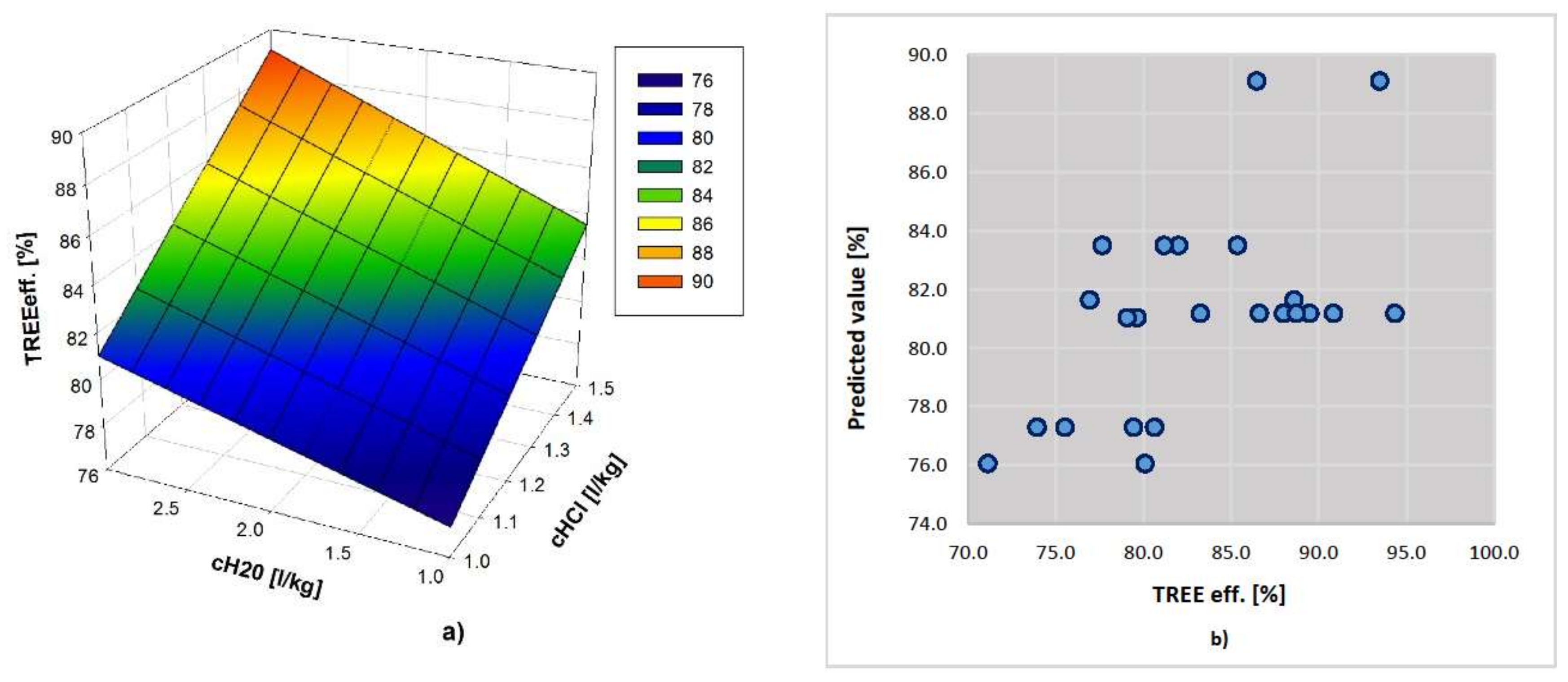
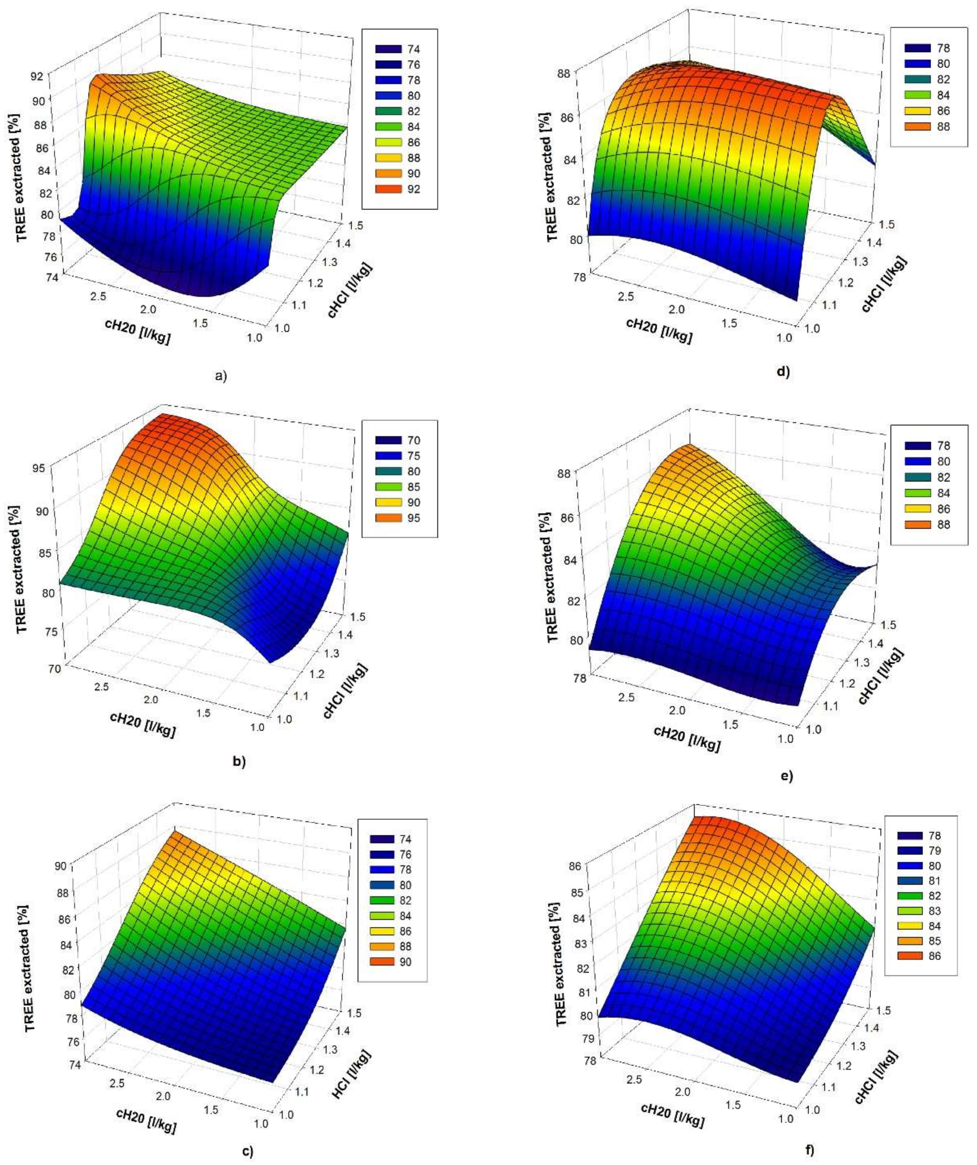
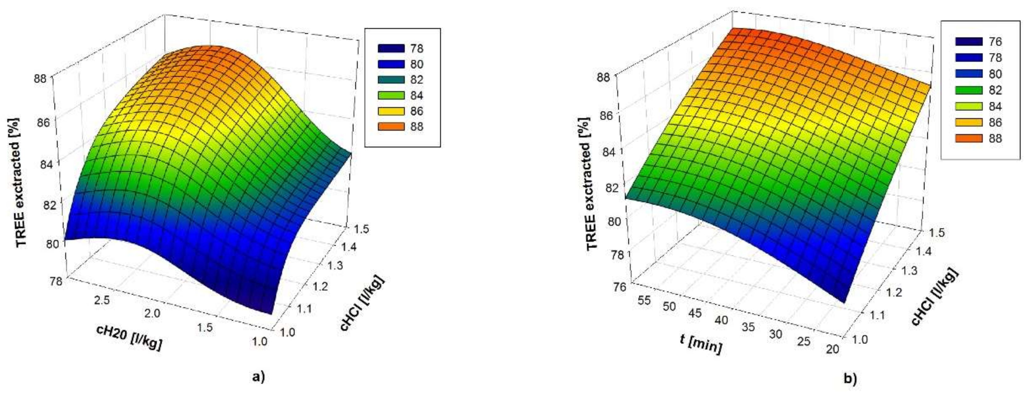
5.3.2. Simulation and Prediction Based on ANN Models

ANN TREE extraction process modeling was implemented on R platform [46], using the neuralnet package. Leave-one Out Cross Validation strategy was implemented in R scripts that were written by authors. The developed ANN modeling strategy, as shown on Figure 10, is completely automated.

For unit (4) (Figure 10) and ANN-4/9/1, BPGD learning algorithm was chosen arbitrarily. Sigmoid function and linear function were used in sequence as the activation functions in the three-layer structure. The learning rate took the value of 0.003 while the momentum constant took the value of 0.9. For unit (5) (Figure 10), and ANN-4/3/2/1, RPROP training algorithm and TANH activation function were chosen. The parameters of the RPROP were ${\eta }^{+}=1.2$ and ${\eta }^{-}=-0.5$, as recommended in references [41,42]. Initial values of weight coefficients were chosen randomly from the range [−0.5, 0.5]. All of the inputs and outputs were normalized in the interval between 0 and 1 by linear scaling. The chosen number of learning epochs was 1000, to avoid overtraining. After 30 repetitions of the modeling process, the most successful result, which was rated by the lowest root mean squared error on single tests points, was chosen as relevant. The error of the adopted model is estimated as the mean RMSE of all the generated ANN models. Performance metric values of the adopted final data table numerical model of REE extraction process (Figure 13), are ${\overline{RMSE}}_{train}=0.856$, for all of the training data sets and ${\overline{RMSE}}_{test}=3.268$, for all the test single points.

The adopted final model (6), depended on four input variables, and its response surface could not be presented in a three-dimensional (3D) diagram. In order to visualize the prediction result, some 3D plots of the response surface were obtained by maintaining some selected factors constant. Some typical diagrams are shown in Figure 13a,b.

6. Validation of the Model and Scale-up

6.1. Validation of REE Extraction Model and Obtained Optimal Process Regimes

In Section 4, the realized CCD plan for dry digestion and the leaching process, was presented. Using the obtained experimental results, mathematical models of the investigated process were created in MLR, SWR, and ANN forms. Final ANN data table numerical model for TREE extraction, given in Figure 13, was adopted as adequate. Based on this model the optimum intervals for the values of predictor variables are determined. These optimized intervals define the optimal regimes for the high performance of the REE extraction process. The optimal intervals for the parameters in stage I and stage II are: hydrochloric acid to concentrate ratio between 1.3 and 1.50, water to concentrate between 2.3–2.5 L/kg, leaching temperature between 20 °C and 25 °C (no external heating), and leaching time between 40 and 60 min. Under these conditions, the model predicted TREE extraction between 86% and 90%. However, considering the cost of REE extraction, in order to obtain and confirm the final values of optimal parameters that would be applied to the pilot scale-up system, some validation experiments were performed in the lab. The operation process was the same as the experiments in the adopted CCD plan. In accordance with the above, four additional experiments were carried out. Each of these four experiments (

Table 5. The results of experiment checking.

Parameter	Units	B1	B2	B3	B4
HCl:Concentrate	L:kg	1.3:1	1.4:1	1.4:1	1.5:1
Water:Concentrate	L:kg	2.25:1	2.25:1	2.5:1	3:1
Leaching time	min	40	50	50	60
Predicted value		85.35%	87.90%	89.40%	89.40%
Actual value		87.65%	89.40%	89.70%	91.20%

) was realized under the same leaching temperature—20 °C.

The mean TREE extraction efficiency for these four experiments, under laboratory conditions, was 89.49% and mean RMSE was RMSE_ANN = 1.65. The obtained results confirmed the adequacy of the adopted ANN model, which was the basis for selecting the optimal regime of the REE extraction technological procedure on the scale-up level.

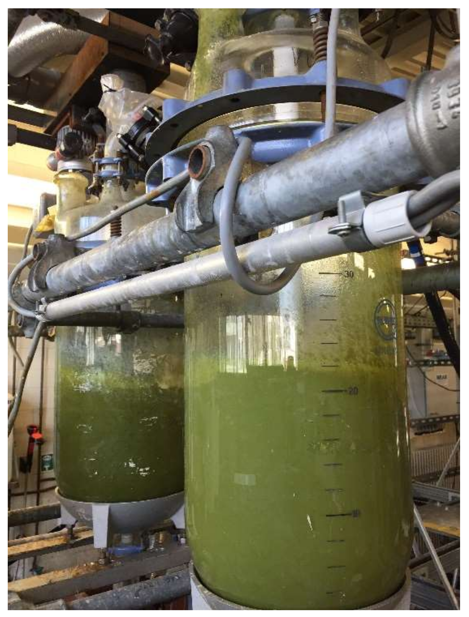
6.2. Dry Digestion and Leaching Process Scale-Up

The laboratory results were validated at one newly built demonstration plant at the IME, RWTH Aachen in order to provide more detailed knowledge of the REE extraction process before industrialization application. Treatment of 500 kg of eudialyte concentrate was performed using two dry digestion reactors (as shown in Figure 14) under the optimal values of process parameters that were obtained using adopted ANN model (Figure 13), described in Section 6.1.

There were two reactors for dry digestion process at the demonstration plant and the capacity of each reactor was 40 L. When considering that the slurry was thick after mixing the acid and eudialyte concentrate, the handling capacity was controlled not to exceed a maximum of 6 kg concentrate per reactor. After performing dry digestion and leaching adding specified amounts of water and transferring the slurry to a large tank (200 L), leaching was then carried out at the temperature of around 20 °C. After neutralization with limestone until the pH reached 4.0, the slurry was pumped to a filter press and the separation of solid and liquid was achieved. The final REE enriched solution was obtained after washing the filter cake, and the composition of the REE enriched solution is shown in

Table 6. Chemical composition of REE enriched solution II in pilot scale-up test.

Element	Concentration (g/L)	Element	Concentration (g/L)
Al	0.56	Ce	0.951
Ca	10.49	Pr	0.105
Fe	2.02	Nd	0.370
Mn	0.269	Sm	0.094
Nb	<0.0001	Gd	0.075
Zr	0.02	Dy	0.105
Hf	0.010	Y	0.601
Si	0.099	Yb	0.069
La	0.425	TREE	2.80

. The experiments were repeated 3–5 times per day. In total, 48 experiments were realized on the scale-up demonstration plant. The mean overall TREE extraction efficiency under adopted optimal regimes defined by model given in Figure 13 was 86.9%.

7. Discussion

7.1. REE Extraction Modeling and Optimal Regimes

The discussion related to the selection of significant predictors in the REE extraction process, the variation intervals of these predictors, the applied CCD experimental plan and the developed mathematical MLR, SWR, and ANN models, with their accuracy and properties, are given in Section 4 and Section 5. The reliability of the ANN model is enhanced by utilizing the LOOCV method. ANN is a nonlinear model capable of incorporating the nonlinear effects of predictor variables and their combined effects on the response variables. This model is also capable to overcome the high levels of noise that characterize the REE extraction process. For these reasons, the adopted ANN model shows better performance and accuracy (${\overline{RMSE}}_{test}=3.268$, ${\overline{RMSE}}_{train}=0.856$) in comparison with MLR ($RMS{E}_{(8)}=4.668$, $R_{adj(8)}^2=0.244$) and SWR ($RMS{E}_{(9)}=4.487$, $R_{adj(9)}^2=0.413$) models.

The validity of the adopted numerical ANN model that is shown in Figure 13 was confirmed under laboratory conditions (Table 5). Optimal variation intervals of the process parameters that predict the maximization of the TREE extraction efficiency from the eudialyte ore (Section 6.1) were determined. As previously described, the expected TREE extraction efficiency is in the range of 86 to 90%.

Tests at the IME RWTH Aachen demonstration plant, under optimal regimes, resulted in an overall average TREE extraction efficiency of 86.9%. The chosen parameter values offer the prevention of silica gel formation. Such results additionally confirm the feasibility of the proposed and designed REE extraction process from eudialyte concentrate and its potential for industrial application. The ratio between concentrate and hydrochloric acid is enough to dissolve rare earth elements from eudialyte concentrate. The leaching time with water between 40 and 60 min is shorter in comparison to the acid baking process and other hydrometallurgical processes under an atmospheric pressure.

Previous models and discussions have indicated that the leaching temperature does not have a significant effect on the TREE extraction efficiency. This fact is of great importance because it has a positive effect both on reducing the costs of REE extraction (no external heating) and on avoiding very complex problems that are related to the types of materials from which reactors and other equipment are made. Additionally, this may have a positive effect on avoiding problems related to corrosion at high temperatures.

To further explore the REE extraction process, additional, potentially significant predictors should be included in the analysis. The first possibly significant predictor, which will be considered in future research, is stirring rate. Potentially, this predictor can influence both the prevention of silica gel formation and the overall duration of the process.

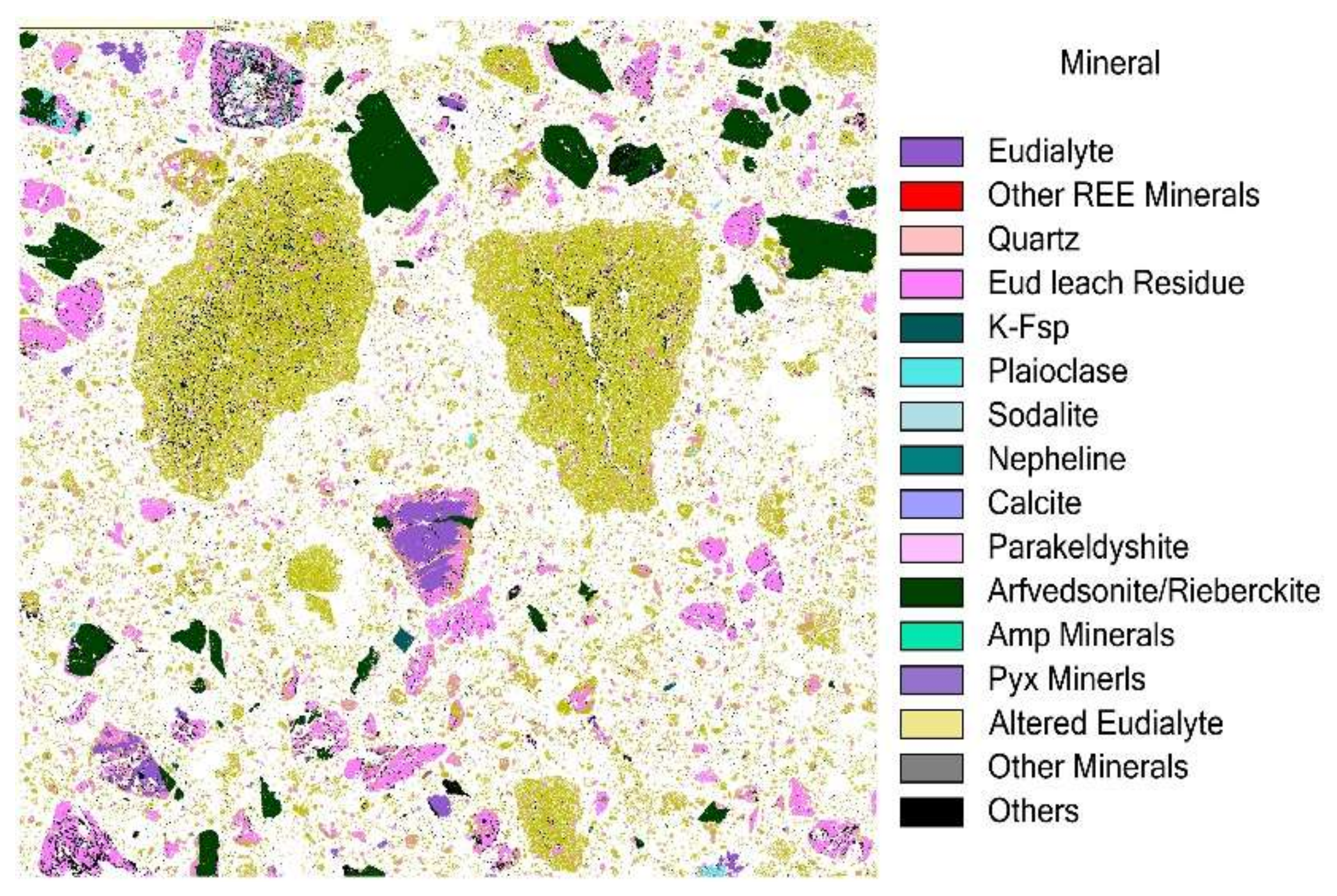
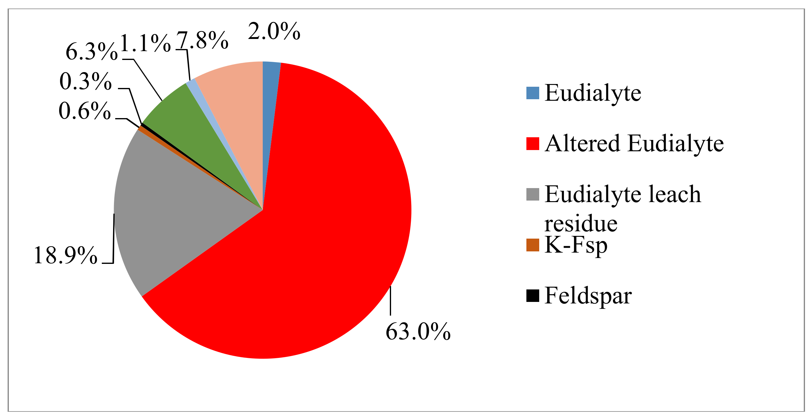
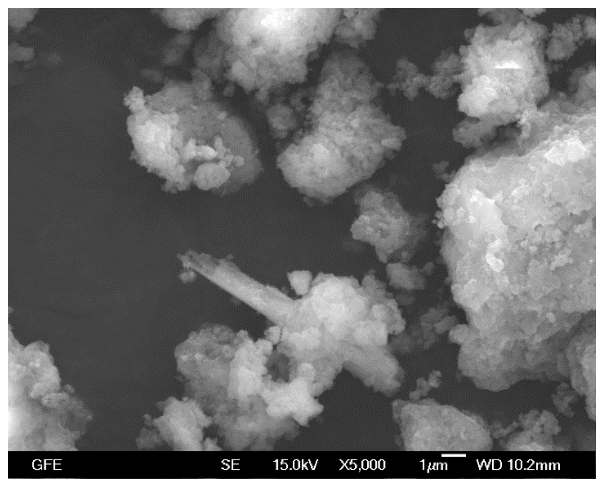
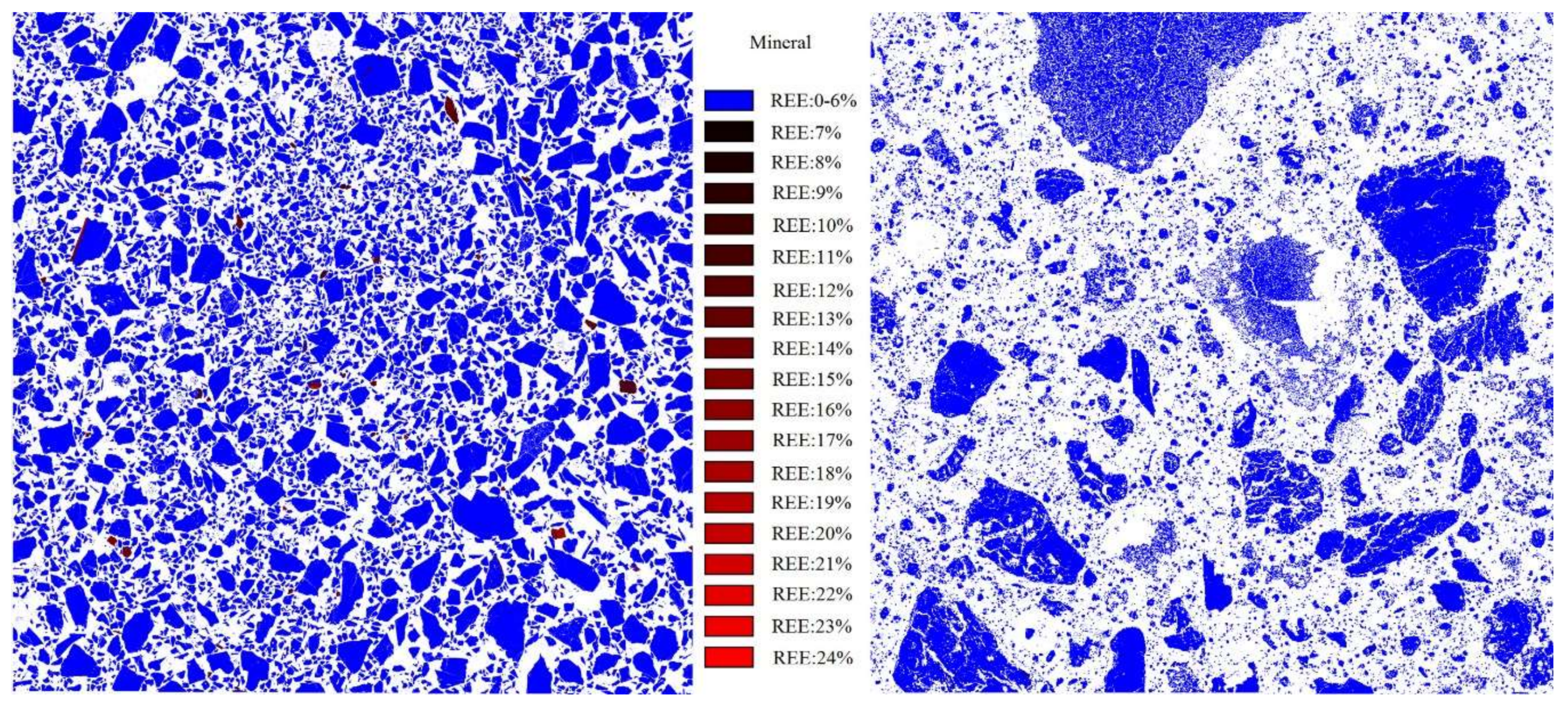
7.2. Phase Changes during REE Extraction

During the REE extraction process there are also phase changes. The analysis and discussion of these changes, in the solid residue, after dry digestion of the eudialyte concentrate with HCl, leaching with water, filtration, and overnight drying, is given in the following text.

As can be seen from Figure 15, the particles of eudialyte leach residue had irregular sizes and the agglomeration of particles could be observed. Figure 16 reveals the mineral composition of the leach residue. Eudialyte residue represented Si-O rich residue phase produced in digestion process, it could not be dissolved into the solution so that the presence of Si in the leaching solution was very low. The SEM result (Figure 17) confirms the same morphological characteristics. It can be explained by the fact that siliceous precipitation formed after HCl treatment can inhibit the leaching of REE. In Figure 18, the REE elemental mapping of eudialyte concentrate and leach residue are given together for the comparison purpose.

The field scan image of eudialyte concentrate in Figure 18 reveals that REE were inhomogeneous and mainly existed in the eudialyte phase. After acid digestion and leaching, few REE was detected in the phases of eudialyte and altered eudialyte.

8. Conclusions

Taking into account the state of the art regarding rare earth elements and the foreseeable, significant increase in the use of REE in various technological domains in the near future, the following assumptions have been made in this study: (a) the REE extraction process from eudialyte concentrate can be carried out at room temperature with a leaching time period that is not exceeding the leaching time periods used in other studies and with an acid concentration that is not higher than the acid concentrations used in other studies, (b) the REE extraction process can, on the basis of an optimal CCD plan, be modeled with a set of suitable MLR, SWR, and/or ANN models, (c) based on the most suitable mathematical model, optimal technological regimes can be determined, which allow for a satisfactory REE extraction efficiency, and (d) a scale-up demonstration plant can verify the feasibility and the efficiency of eudialyte concentrate treatment at low leaching temperatures.

The novelty in this study is the application of the DOE paradigm, the CCD optimal design of experiments, and the creation of a number of mathematical MLR, SWR, or ANN models, which more deeply describe the REE extraction process from eudialyte concentrate. Based on the realized CCD plan under laboratory conditions, various MLR, SWR, and ANN models of dry digestion and leaching process were created and used to predict the effects of various parameters such as hydrochloric acid to eudialyte concentrate ratio, water for leaching to eudialyte concentrate ratio, leaching temperature, and leaching time on the TREE extraction efficiency. The ANN model, which is based on LOOCV, was selected as the most suitable by the authors of this paper. ANN is a nonlinear model capable of incorporating the nonlinear effects of predictor variables and their combined effects on the response variables. This model is also capable to overcome the high levels of noise that characterize the REE extraction process. The reliability of the ANN model is improved with the use of the LOOCV method. For these reasons, the adopted ANN model shows better performance and in comparison with and SWR models. This approach for the extraction of rare earth elements during dry digestion and leaching process is missing in literature, and not present in previous work of Voßenkaul [24]. The research reported in this paper, also as a novelty, explored the feasibility and efficiency of the REE extraction process at room temperature on a scale-up demonstration platform that precedes future industrial application. Information on upscaling operations for treatment of eudialyte is also missing in overall literature.

In this study, it was confirmed that the proposed process is capable of achieving high REE recovery from an eudialyte concentrate during dry digestion with hydrochloric acid and leaching with water, avoiding silica gel formation and lowering operation costs (no heating for dry digestion and leaching). Based on the modeling results (as shown in Figure 13a,b), the optimal parameters in stage I and stage II are: hydrochloric acid to concentrate ratio between 1.3 and 1.50, water to concentrate between 2.3 and 2.5 L/kg, leaching temperature between 20 °C and 25 °C (no external heating), leaching time between 40 and 60 min. Finally, using the four parameters from the optimal range, the scale-up test was conducted at the IME-demonstration plant and the overall efficiency of the TREE extraction was 86.90%, which confirmed the feasibility and achieved good performance.

In comparison to the other process with sulphuric acid: Acid baking (250–300 °C; duration 2–4 h) [49] and Kvanefjeld process (80–95 °C, with a duration of approximately 16 h for the first and second leaching phase) [50], our REE extraction process is an environmentally friendly process, at room temperature, with a duration of approximately 2 h. During our research, we found that the leaching temperature has no significant influence on the increase of the extraction efficiency. Consequently, our proposed process is cheaper than other mentioned processes.

The obtained results are very promising, and will be used in our future work in order to propose and design a new dry digestion reactor (approximate volume 100 L) for an industrial application. This reactor might be used, not only for the treatment of a eudialyte concentrate, but also for a Bauxite residues (red mud) from the aluminum industry, what is mentioned in our newest publication in Nature [25]. Our future research will also take into consideration the stirring rate as one of the possibly important parameters regarding the avoidance of gel formation, leaching efficiency, and the duration of the REE extraction process.

References

1. Thomas, P.J.; Carpenter, D.; Boutin, C.; Allison, J.E. Rare earth elements (REEs): Effects on germination and growth of selected crop and native plant species. Chemosphere 2014, 96, 57–66. [Google Scholar] [CrossRef] [PubMed]
2. Morais, C.A.; Ciminelli, V.S.T. Process development for the recovery of high-grade lanthanum by solvent extraction. Hydrometallurgy 2004, 73, 237–244. [Google Scholar] [CrossRef]
3. Maestro, P.; Huguenin, D. Industrial applications of rare earths: Which way for the end of the century? J. Alloys Compd. 1995, 225, 520–528. [Google Scholar] [CrossRef]
4. Krishnamurthy, N.; Gupta, C.K. The Rare Earths, Extractive Metallurgy of Rare Earths; CRC Press: Boca Raton, FL, USA, 2015; pp. 1–84. [Google Scholar]
5. Hoshino, M.; Sanematsu, K.; Watanabe, Y. REE mineralogy and resources. In Handbook on the Physics and Chemistry of Rare Earths; Elsevier: New York, NY, USA, 2016; Volume 49, pp. 129–291. [Google Scholar]
6. McLemore, V.T. Rare earth elements (REE) deposits associated with great plain margin deposits (alkaline-related), southwestern united states and eastern mexico. Resources 2018, 7, 8. [Google Scholar] [CrossRef]
7. Möller, V.; Williams-Jones, A.E. A hyperspectral study (V-NIR-SWIR) of the Nechalacho REE-Nb-Zr deposit, Canada. J. Geochem. Explor. 2018, 188, 194–215. [Google Scholar] [CrossRef]
8. Alonso, E.; Sherman, A.M.; Wallington, T.J.; Everson, M.P.; Field, F.R.; Roth, R.; Kirchain, R.E. Evaluating rare earth element availability: A case with revolutionary demand from clean technologies. Environ. Sci. Technol. 2012, 46, 3406–3414. [Google Scholar] [CrossRef] [PubMed]
9. Golev, A.; Scott, M.; Erskine, P.D.; Ali, S.H.; Ballantyne, G.R. Rare earths supply chains: Current status, constraints and opportunities. Resour. Policy 2014, 41, 52–59. [Google Scholar] [CrossRef]
10. Goodenough, K.; Schilling, J.; Jonsson, E.; Kalvig, P.; Charles, N.; Tuduri, J.; Deady, E.; Sadeghi, M.; Schiellerup, H.; Müller, A. Europe’s rare earth element resource potential: An overview of REE metallogenetic provinces and their geodynamic setting. Ore Geol. Rev. 2016, 72, 838–856. [Google Scholar] [CrossRef]
11. Balomenos, E.; Davris, P.; Deady, E.; Yang, J.; Panias, D.; Friedrich, B.; Binnemans, K.; Seisenbaeva, G.; Dittrich, C.; Kalvig, P. The EURARE project: Development of a sustainable exploitation scheme for Europe’s Rare Earth Ore deposits. Johns. Matthey Technol. Rev. 2017, 61, 142–153. [Google Scholar] [CrossRef]
12. García, M.V.R.; Krzemień, A.; Del Campo, M.Á.M.; Álvarez, M.M.; Gent, M.R. Rare earth elements mining investment: It is not all about China. Resour. Policy 2017, 53, 66–76. [Google Scholar] [CrossRef]
13. Torró, L.; Proenza, J.; Aiglsperger, T.; Bover-Arnal, T.; Villanova-de-Benavent, C.; Rodríguez-García, D.; Ramírez, A.; Rodríguez, J.; Mosquea, L.; Salas, R. Geological, geochemical and mineralogical characteristics of REE-bearing Las Mercedes bauxite deposit, Dominican Republic. Ore Geol. Rev. 2017, 89, 114–131. [Google Scholar] [CrossRef]
14. Edahbi, M.; Benzaazoua, M.; Plante, B.; Doire, S.; Kormos, L. Mineralogical characterization using QEMSCAN® and leaching potential study of REE within silicate ores: A case study of the Matamec project, Québec, Canada. J. Geochem. Explor. 2018, 185, 64–73. [Google Scholar] [CrossRef]
15. Mikhailova, J.; Pakhomovsky, Y.A.; Ivanyuk, G.Y.; Bazai, A.; Yakovenchuk, V.; Elizarova, I.; Kalashnikov, A. REE mineralogy and geochemistry of the Western Keivy peralkaline granite massif, Kola Peninsula, Russia. Ore Geol. Rev. 2017, 82, 181–197. [Google Scholar] [CrossRef]
16. Deymar, S.; Yazdi, M.; Rezvanianzadeh, M.R.; Behzadi, M. Alkali metasomatism as a process for Ti–REE–Y–U–Th mineralization in the Saghand Anomaly 5, Central Iran: Insights from geochemical, mineralogical, and stable isotope data. Ore Geol. Rev. 2018, 93, 308–336. [Google Scholar] [CrossRef]
17. Davris, P.; Stopic, S.; Balomenos, E.; Panias, D.; Paspaliaris, I.; Friedrich, B. Leaching of rare earth elements from eudialyte concentrate by suppressing silica gel formation. Miner. Eng. 2017, 108, 115–122. [Google Scholar] [CrossRef]
18. Borst, A.M.; Friis, H.; Andersen, T.; Nielsen, T.; Waight, T.E.; Smit, M.A. Zirconosilicates in the kakortokites of the Ilímaussaq complex, South Greenland: Implications for fluid evolution and high-field-strength and rare-earth element mineralization in agpaitic systems. Miner. Mag. 2016, 80, 5–30. [Google Scholar] [CrossRef]
19. Anthony, J.W.; Bideaux, R.A.; Bladh, K.W.; Nichols, M.C. Handbook of Mineralogy, Volume IV, Arsenates, Phosphates, Vanadates; Mineralogical Society of America: Chantilly, VA, USA, 2000. [Google Scholar]
20. Johnsen, O.; Ferraris, G.; Gault, R.A.; Grice, J.D.; Kampf, A.R.; Pekov, I.V. The nomenclature of eudialyte-group minerals. Can. Miner. 2003, 41, 785–794. [Google Scholar] [CrossRef]
21. Zakharov, V.; Maiorov, D.; Alishkin, A.; Matveev, V. Causes of insufficient recovery of zirconium during acidic processing of lovozero eudialyte concentrate. Rus. J. Non-Ferr. Met. 2011, 52, 423–428. [Google Scholar] [CrossRef]
22. Lebedev, V. Sulfuric acid technology for processing of eudialyte concentrate. Rus. J. Appl. Chem. 2003, 76, 1559–1563. [Google Scholar] [CrossRef]
23. Lebedev, V.; Shchur, T.; Maiorov, D.; Popova, L.; Serkova, R. Specific features of acid decomposition of eudialyte and certain rare-metal concentrates from Kola peninsula. Rus. J. Appl. Chem. 2003, 76, 1191–1196. [Google Scholar] [CrossRef]
24. Voßenkaul, D.; Birich, A.; Müller, N.; Stoltz, N.; Friedrich, B. Hydrometallurgical processing of eudialyte bearing concentrates to recover rare earth elements via low-temperature dry digestion to prevent the silica gel formation. J. Sustain. Metall. 2017, 3, 79–89. [Google Scholar] [CrossRef]
25. Alkan, G.; Yagmurlu, B.; Cakmakoglu, S.; Hertel, T.; Kaya, Ş.; Gronen, L.; Stopic, S.; Friedrich, B. Novel Approach for Enhanced Scandium and Titanium Leaching Efficiency from Bauxite Residue with Suppressed Silica Gel Formation. Nat. Sci. Rep. 2018, 8, 5676. [Google Scholar] [CrossRef] [PubMed]
26. Vaccarezza, V.; Anderson, C. Beneficiation and Leaching Study of Norra Kärr Eudialyte Mineral; TMS Annual Meeting & Exhibition; Springer: Berlin, Germany, 2018; pp. 39–51. [Google Scholar]
27. Rivera, R.M.; Ulenaers, B.; Ounoughene, G.; Binnemans, K.; Van Gerven, T. Extraction of rare earths from bauxite residue (red mud) by dry digestion followed by water leaching. Miner. Eng. 2018, 119, 82–92. [Google Scholar] [CrossRef]
28. Milivojevic, M.; Stopic, S.; Friedrich, B.; Stojanovic, B.; Drndarevic, D. Computer modeling of high-pressure leaching process of nickel laterite by design of experiments and neural networks. Int. J. Miner. Metall. Mater. 2012, 19, 584–594. [Google Scholar] [CrossRef]
29. Milivojevic, M.; Stopic, S.; Stojanovic, B.; Drndarevic, D.; Bernd, F. Forward stepwise regression in determining dimensions of forming and sizing tools for self-lubricated bearings. METALL 2013, 67, 92–98. [Google Scholar]
30. Mata, J. Interpretation of concrete dam behaviour with artificial neural network and multiple linear regression models. Eng. Struct. 2011, 33, 903–910. [Google Scholar] [CrossRef]
31. Cohen, J.; Cohen, P.; West, S.G.; Aiken, L.S. Applied Multiple Regression/Correlation Analysis for the Behavioral Sciences; Routledge: Abingdon, UK, 2013. [Google Scholar]
32. Fisher, R.A. The Design of Experiments; Oliver and Boyd: Edinburgh, UK; London, UK, 1937. [Google Scholar]
33. Box, G.E.; Wilson, K.B. On the experimental attainment of optimum conditions. In Breakthroughs in Statistics; Springer: Berlin, Germany, 1992; pp. 270–310. [Google Scholar]
34. Dong, L.; Park, K.-H.; Zhan, W.; Guo, X.-Y. Response surface design for nickel recovery from laterite by sulfation-roasting-leaching process. Trans. Nonferr. Met. Soc. China 2010, 20, s92–s96. [Google Scholar]
35. Rumelhalt, D. Learning Internal Representation by Error Propogation, Parallel Distributed Processing: Explorations in the Microstructure of Cognition (Vol. 1); MIT Press: Cambridge, MA, USA, 1986. [Google Scholar]
36. Drndarevic, D. Modeling and Optimization of Powder Metallurgy Process by Neural Networks. Ph.D. Thesis, University of Belgrade, Beograd, Serbia, 1996. [Google Scholar]
37. Law, R. Back-propagation learning in improving the accuracy of neural network-based tourism demand forecasting. Tour. Manag. 2000, 21, 331–340. [Google Scholar] [CrossRef]
38. Majdi, A.; Beiki, M. Evolving neural network using a genetic algorithm for predicting the deformation modulus of rock masses. Int. J. Rock Mech. Min. Sci. 2010, 47, 246–253. [Google Scholar] [CrossRef]
39. Yu, Z. Feed-Forward Neural Networks and Their Applications in Forecasting; University of Houston: Houston, TX, USA, 2000. [Google Scholar]
40. Heaton, J. Programming Neural Networks with Encog 3 in c#; Heaton Research, Inc.: St. Louis, MI, USA, 2015. [Google Scholar]
41. Riedmiller, M.; Braun, H. A Direct Adaptive Method for Faster Backpropagation Learning: The RPROP algorithm. In Proceedings of the IEEE International Conference on Neural Networks, San Francisco, CA, USA, 28 March–1 April 1993; pp. 586–591. [Google Scholar]
42. Riedmiller, M. Advanced supervised learning in multi-layer perceptrons—From backpropagation to adaptive learning algorithms. Comput. Stand. Interfaces 1994, 16, 265–278. [Google Scholar] [CrossRef]
43. Kingma, D.P.; Ba, J. Adam: A method for stochastic optimization. arXiv. 2014. arXiv.org e-Print archive. Available online: https://arxiv.org/abs/1412.6980 (accessed on 22 December 2014).
44. Milivojević, M. Methods of Development and Adaptation of Regression Models Based on Genetic Algorithms. Ph.D. Thesis, University of Kragujevac, Kragujevac, Serbia, 2016. [Google Scholar]
45. Pallant, J. SPSS Survival Manual, 3rd ed.; Mc Graw Hill: New York, NY, USA, 2007. [Google Scholar]
46. Team, R. RR Development Core Team: A Language and Environment for Statistical Computing; R Foundation for Statistical Computing: Vienna, Austria, 2012; ISBN 3-900051-07-0. [Google Scholar]
47. Hecht-Nielsen, R. Kolmogorov’s mapping neural network existence theorem. In Proceedings of the International Conference on Neural Networks, San Diego, CA, USA, 21–24 June 1987; pp. 11–14. [Google Scholar]
48. McCaffrey, J. Understanding and using K-fold cross validation for neural networks. Visual Studio Magazine, 24 October 2013. [Google Scholar]
49. Sadri, F.; Nazari, A.M.; Ghahreman, A. A review on the cracking, baking and leaching processes of rare earth element concentrates. J. Rare Earths 2017, 35, 739–752. [Google Scholar] [CrossRef]
50. Krebs, D.; Furfaro, D. Processing of Rare Earth and Uranium Containing Ores and Concentrates. Patent WO 2014/082113 A1, 5 June 2014. [Google Scholar]
Figure 1. Arrangement of experimental points in 2k space: (a) k = 3; (b) k = 3, alpha = 1.682.
Metals 08 00267 g001
Figure 2. Schematic view of a feed-forward Artificial Neural Network (ANN).
Metals 08 00267 g002
Figure 3. Supervised learning model.
Metals 08 00267 g003
Figure 4. QEMSCAN analysis of eudialyte concentrate ((left) false color image after evaluation, (right) initial BSE-image).
Metals 08 00267 g004
Figure 5. Mineral distribution of eudialyte concentrate (analysis by GTK, Finnland).
Metals 08 00267 g005
Figure 6. Proposed flowchart of the treatment of rare earth elements (REE) extraction from eudialyte concentrate.
Metals 08 00267 g006
Figure 7. TREEeff. = f(cHCl, cH2O) for (a) T = const. = 20 °C, t = const. = 20 min.; and, (b) T = const. = 20 °C, t = const. = 60 min.
Metals 08 00267 g007
Figure 8. (a) Total rare earth elements (TREE) extraction model; and, (b) Predicted by Observed plot for TREEeff.
Metals 08 00267 g008
Figure 9. ANN TREE extraction modeling.
Metals 08 00267 g009
Figure 10. ANN topology for TREE modeling: (a) ANN-4/10/1; and, (b) ANN-4/3/2/1.
Metals 08 00267 g010
Figure 11. Leave-one-out Cross Validation in ANN modeling.
Metals 08 00267 g011
Figure 12. Examples of ANN models obtained during the leave-one-out cross validation (LOO CV) process: (a) ANN-4/3/2/1 model: excluded sample A4; (b) ANN-4/3/2/1 model: excluded sample A5; (c) ANN-4/3/2/1 model: excluded sample A10; (d) ANN-4/10/1 model: excluded sample A2; (e) ANN-4/10/1 model: excluded sample A10; and, (f) ANN-4/10/1 model: excluded sample A16.
Metals 08 00267 g012
Figure 13. Final ANN data table numerical model for TREE extraction: (a) T = 20 °C = const., t = 60 min. = const.; (b) T = 20 °C = const., cH2O = 1.5 L/kg = const.
Metals 08 00267 g013
Figure 14. Treatment of eudialyte concentrate in two reactors at the Institute of Process Metallurgy and Metal Recycling (IME) demonstration plant, RWTH Aachen.
Metals 08 00267 g014
Figure 15. QEMSCAN analysis of eudialyte leach residue.
Metals 08 00267 g015
Figure 16. Mineral distribution of a eudialyte leach residue.
Metals 08 00267 g016
Figure 17. SEM image of a eudialyte leach residue.
Metals 08 00267 g017
Figure 18. REE elemental mapping of eudialyte concentrate and leach residue by QEMSCAN.
Metals 08 00267 g018