Article

Evaluation Study on Iterative Inverse Modeling Procedure for Determining Post-Necking Hardening Behavior of Sheet Metal at Elevated Temperature

1
School of Energy and Power Engineering, Beihang University, Beijing 100191, China
2
Collaborative Innovation Center of Advanced Aero-Engine, Beijing 100191, China
3
School of Mechanical Engineering and Automation, Beihang University, Beijing 100191, China
*
Author to whom correspondence should be addressed.
Metals 2018, 8(12), 1044; https://doi.org/10.3390/met8121044
Submission received: 13 November 2018 / Revised: 30 November 2018 / Accepted: 5 December 2018 / Published: 10 December 2018
(This article belongs to the Special Issue Failure Mechanisms in Alloys)

Abstract

:
The identification of the post-necking strain hardening behavior of metal sheet is important for finite element analysis procedures of sheet metal forming process. The inverse modeling method is a practical way to determine the hardening curve to large strains. This study is thus focused on the evaluation of the inverse modeling method using a novel material performance test. In this article, hot uniaxial tensile test of a commercially pure titanium sheet with rectangular section was first conducted. Utilizing the raw data from the tensile test, the post-necking hardening behavior of the material is determined by a FE-based inverse modeling procedure. Then the inverse method is compared with some classical hardening models. In order to further evaluate the applicability of the inverse method, biaxial tensile test at elevated temperatures was performed using a special designed cruciform specimen. The cruciform specimen could guarantee that the maximum equi-biaxial deformation occurs in the center section. By using the inverse modeling procedure, the hardening curves under biaxial stress state are able to be extracted. Finally the stress-strain curves obtained from the two experiments are compared and analysis studies are provided.

1. Introduction

Nowadays the Finite Element Analysis (FEA) is used widely in the design stage of sheet metal forming operations with the aim of reducing the number of trial steps, controlling dimension accuracy and finally obtaining high-quality sheet forming products [1] and is almost indispensable in the manufacturing industries. The simulation of metal forming process is a highly non-linear problem involving large material deformation and complex boundary conditions [2] which requires accurate hardening behavior of the investigated sheet metal over a wide range of plastic strains. Till now the most popular method to obtain the stress-strain relationship of metal sheet, represented either in the form of a set of discrete data points or analytical constitutive models, is typically by conducting standard uniaxial tensile test with rectangular cross-section [3,4]. The stress and strain values of the uniaxial tensile test can be obtained by using an extensometer that measures the elongation of a certain gauge length but the calculated stress value is accurate on the assumption that the test specimen is subjected to homogeneous state of uniaxial loading, which means that the stress-strain relationship identified by standard uniaxial tensile test is valid only before the so-called diffuse necking point. However, many sheet forming processes usually involve large deformation and can generate strains far beyond the necking point, so the stress-strain curve up to the necking point is not sufficient for numerical simulation procedures. Generally, the available pre-necking stress-strain curves are extrapolated to large strains using different hardening models [5]. It is obvious that the predicted post-necking hardening curve greatly depends on the choice of phenomenological constitutive models and one model that is best fitted to a certain material may not suits for another [6].
Recently, numerous investigations have been made to acquire the hardening curve beyond diffuse necking by many researchers [7,8,9,10,11]. The initial attempt was made by Bridgman [7], who derived a set of analytical models for the distribution of stress and strain across the diffuse necking region for a round bar. However, the correction and compensation for stress and stress values of Bridgman’s method is based on the measurement of evolving geometrical parameters of the necking area, which requires much experimental effort. Ling [8] and Zhang et al. [9] extended the research of Bridgman by proposing new models for determining the post-necking hardening behavior of strip specimen with rectangular section. Other researchers [10,11] further studied the necking problem experimentally based on Bridgman’s work in more sophisticated ways. Currently, a new optical-numerical measurement techniques, i.e., the Digital Image Correlation (DIC) method, is used widely for obtaining full-field information for both in-plane displacements and strains of the test specimen and has been applied by many researchers for determining the post-necking hardening curve of uniaxial test [12,13], Scheider et al. [14] investigated the necking phenomenon based on finite element analysis with the help of DIC technique and proposed a new post-necking model which has a higher accuracy than Zhang’s [9] model. Another effort to identify the post-necking stress-strain curve of uniaxial tensile test is concentrated on the inverse modeling procedures. In most cases, the stress-strain points or the unknown parameters of constitutive model are determined iteratively with the help of FEA or the Virtual Fields Method (VFM). The finite element based inverse method is perhaps the most popular way in the iterative modeling procedures for determining stress-strain curve after necking and substantial studies are focused on it. Kajberg et al. [2] combined inverse modeling with in-plane displacement fields measured by DIC method and determined the parameters of parabolic hardening model beyond necking point. Kamaya et al. [15] determined the stress–strain curve including post-necking strain using hourglass type specimens of different notch radius. Faurholdt [16] and Koc [17] respectively designed a least-square cost function which represents the discrepancy between the experimental result and the FEM computed response. Other researchers [3,18,19] focus on the non-linear VFM which could replace finite element method in the inverse modeling process. The key point of VFM is to determine the hardening behavior by minimizing the discrepancy between the internal and the external work in the region where the diffuse neck develops [3]. The VFM-based inverse method was first proposed by Coppieters et al. [6] who identified the parameters of the Voce and the Swift hardening laws for a mild deep drawing steel using tensile test data from the pre- and post-necking region. Rossi et al. [18] presented a VFM-based procedure to extract the constitutive parameters of a plasticity model at large plastic strains using three dimensional displacement field. The proposed procedure method was then validated by conducting finite element simulation of uniaxial tensile test. Due to the insufficient accuracy of the common hardening laws when implementing VFM-based inverse modeling process, Coppieters et al. [3] proposed a p-model which can reflect the accurate stress-strain relationship both in the pre- and post-necking region of a cold rolled interstitial-free steel sheet. Kim et al. [19] applied the diffuse approximation (DA) method to decrease the noise effect from the measured full-field displacements when characterizing the post-necking strain hardening behavior using VFM.
The FE-based and VFM-based method have been experimentally validated in the pre-necking regime of uniaxial tensile test [20,21]. However, the evaluation of the inverse modeling methods by an independent material test is much more difficult and is currently lacking [3], as in a tensile test, the true strain at the smallest cross-section in the necked region may exceed 1.5 just before ductile fracture happens [20]. So it is important to select a material performance test capable of achieving very large strains under uniform deformation. Coppieters et al. [3,22] used the multi-axial tube expansion test designed by Kuwabara and Sugawara [23] to acquire uniaxial strain hardening behavior beyond necking point for the validation study of the VFM-based method and good agreement was obtained. However, very few investigation concentrates on the evaluation test at relatively high temperatures, which is a main target of this research.
This study is focused on the evaluation of the inverse modeling method using a novel material performance test at elevated temperature. In this article, hot uniaxial tensile test of a commercially pure titanium sheet with rectangular section was first conducted. Utilizing the raw data from the tensile test, the post-necking hardening behavior of the material is determined by an FE-based inverse modeling procedure. In order to further evaluate the applicability of the inverse method, biaxial tensile test at elevated temperature was performed using a special designed cruciform specimen. The cruciform specimen could guarantee that the maximum equi-biaxial deformation occurs in the center section. By using the inverse modeling procedure, the hardening curves under biaxial stress state are able to be extracted. Finally the stress-strain curves obtained from the two experiments are compared and analysis studies are provided.

2. Inverse Modeling Method

2.1. Experimental Details

The material used in this study is a commercial pure titanium (Grade 2). The titanium and Ti-alloys are well known for their high strength-to-weight ratio, good heat and corrosion resistance [24], and are used widely for high quality thin-walled components [25]. Specimens used in the hot tensile test were machined by wire-electrode cutting with the geometry of the specimen illustrated in Figure 1. The isothermal tensile tests were conducted on a ZWICK universal testing machine (constant-speed loading, the maximum load capacity is 20 kN) at 500 °C and three different strain rates, 0.1 s−1, 0.02 s−1, 0.005 s−1. For a uniform temperature distribution, all specimens were held for 5 min before deformation. The raw data from the hot tensile test of traction force versus elongation is plotted in Figure 2. It is obvious from the figure that the tensile test specimen has a larger elongation and a smaller maximum traction force when the deformation speed is lower, which is a typical character for the titanium at elevated temperatures.

2.2. FE-Based Inverse Modeling Procedure

An Epsilon high temperature extensometer was used in the tensile test to measure the uniform deformation of the specimen, but the stress-strain curve of the material after necking is no longer reliable and is thus calculated by an FE-based inverse modeling procedure in this research. Many researchers [2,4,20] have proposed several FE-based inverse methods respectively and we used a modified inverse method based on the early work of Joun [20].
By utilizing the commercial finite element software ABAQUS, the uniaxial tensile test can be simulated and the force and elongation of the specimen can be calculated, so the main idea of the inverse method is to iteratively improve the input stress-strain data of the numerical model to better conform to the measured force and elongation { P i e x , U i e x } from the experiment. Supposing at the Nth iterative step, the modified input stress-plastic strain data is ( σ N , ε N ) , where σ N = { σ i } N and ε N = { ε i p l } N , i stands for each point of the hardening curve. When the largest plastic strain in the specimen reaches a certain value of ε i , the calculated reaction force and elongation by FEM simulation are represented here as P i F E and U i F E respectively. In order to reduce the difference between the calculated and measured force P i F E , P i e x at the same elongation U i e x = U i F E , the stress update algorithm as expressed in Equation (1) is adopted [20] to calculate the new iterative stress value corresponding to the plastic strain ε i .
σ i n e w = σ i o l d · P i e x / P i F E
A schematic diagram of the inverse method is shown in Figure 3, and the iterative procedure can be summarized in the following:
(1)
The initial guess of the stress-plastic strain data { σ i N , ε i N } (N = 1) pre-necking point is obtained from the experiment using an extensometer. Although the measured hardening curve by using extensometer has been proved accurate by some researchers [19], the iterative optimization method in this research still covers both pre- and post-necking region of the hardening curve to further exam the reliability of the inverse method.
(2)
By conducting FEM simulation, the traction force and elongation of the specimen at the Nth step can be calculated as { P i , N F E , U i , N F E } . In order to compare the simulation result with the experiment, the experimental force value P i e x at the same U i , N F E = U i e x is determined by interpolation. By comparing the measured force P i e x and predicted force P i , N F E , the improved stress at plastic strain ε i N is corrected as σ i N + 1 = σ i N · P i e x / P i , N F E .
(3)
Calculate the new simulation model using the updated input hardening curve { σ i N + 1 , ε i N + 1 } and extract the (N + 1)th force and elongation data of the specimen { P i , N + 1 F E , U i , N + 1 F E } .
(4)
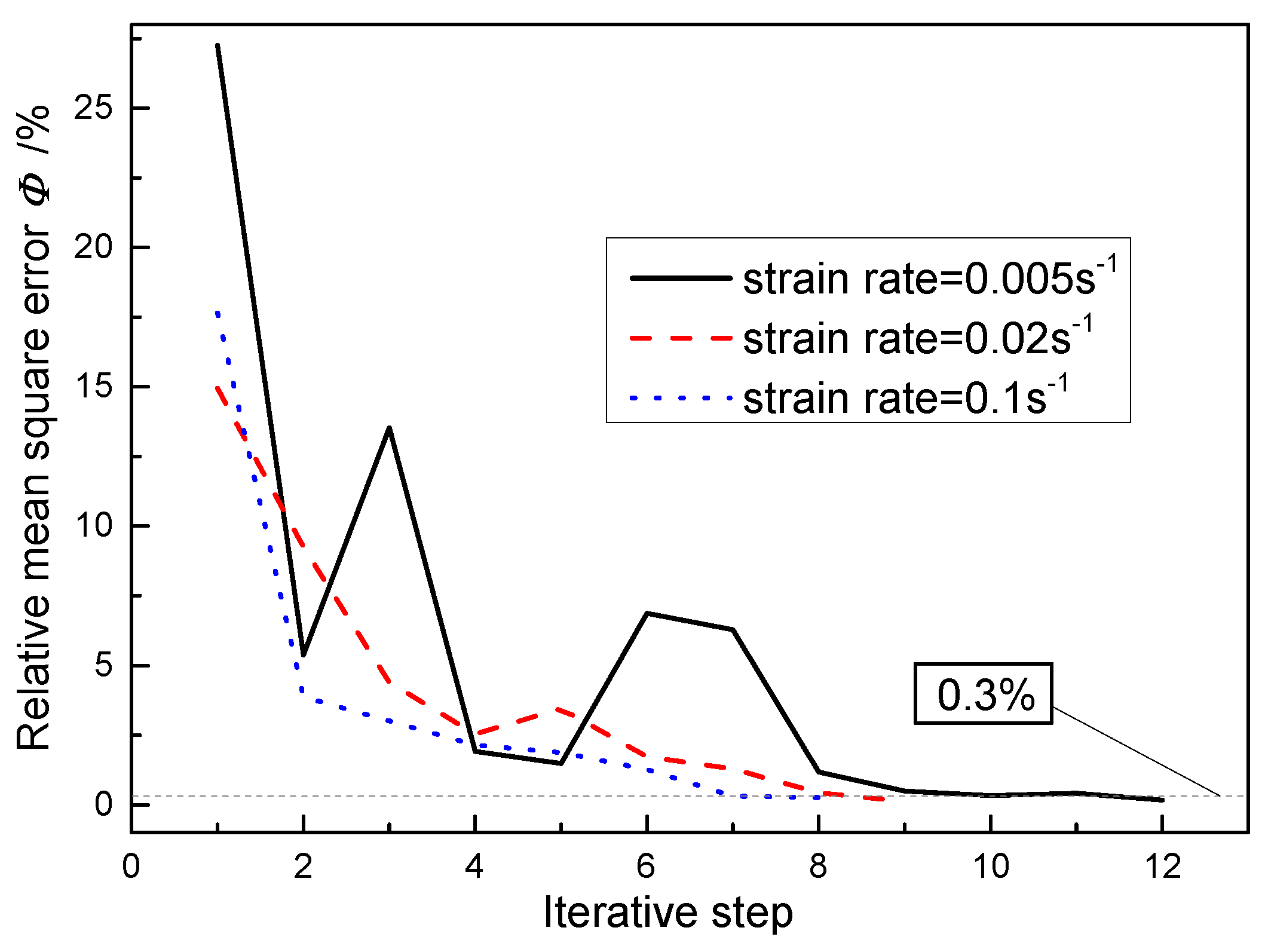
After several iterative steps, the predicted force and elongation data will get close to the experimental result. In order to evaluate the discrepancy between the calculated and the measured data, the relative mean square error Φ is calculated in this research, which has the expression as described in Equation (2).
Φ = ( P i , N F E P i e x ) 2 / M / ( P i e x / M )
where M is the total number of the data points.
(5)
If the relative mean square error Φ is lower than 0.3%, the last stress-plastic strain data { σ i N , ε i N } is then regarded as the final effective hardening curve determined by the inverse modeling method, else go back to step (2).
Throughout the inverse modeling procedure, the elongation and traction force of the specimen are the only two necessary measured data sets from uniaxial tensile test, which are easy to be obtained. However, there is a problem arise from this method: When the elongation of the specimen gets to the value of U i e x in the tensile test, the actual maximum plastic strain in the specimen is denoted as ε i e x here, but without the application of the DIC method, the ε i e x value cannot be determined from experiment, then the stress value σ i N in the numerical simulation is corrected using Equation (1) at the elongation U i F E = U i e x corresponding to plastic strain ε i N which may be different from the ε i e x value. But it will be discovered later that this discrepancy between the two plastic strain values from experiment and simulation is not important for the final convergence and accuracy of the determined hardening curve, which will be introduced in Section 3.

3. Analysis of the Method

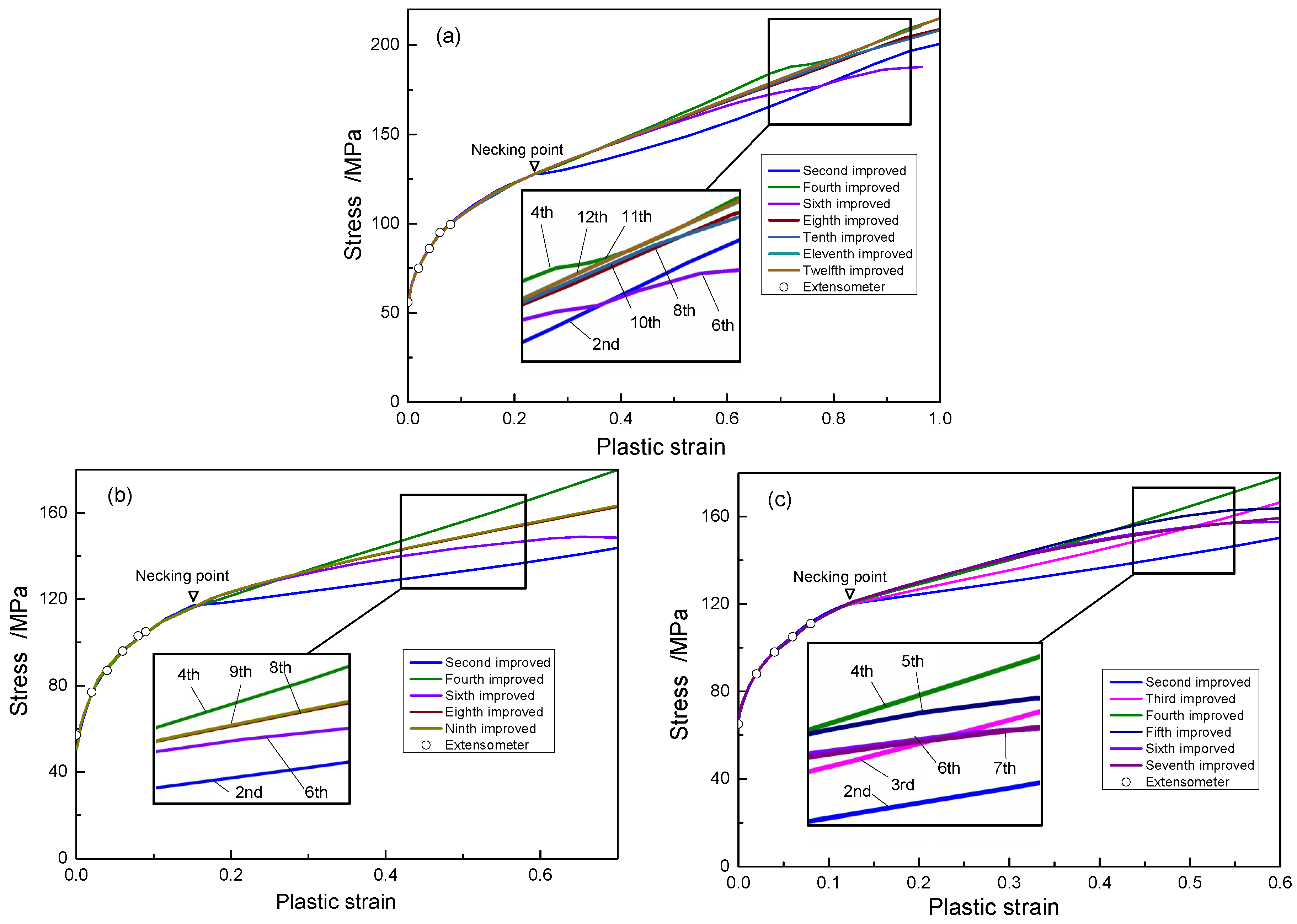
3.1. Convergence Analysis

The improved stress-plastic strain curves of some iterative steps by the inverse modeling method at different strain rates are illustrated in Figure 4. It is obvious from the figure that the stress-strain data measured by the extensometer is identical with the pre-necking curve obtained by the inverse method, which means that the inverse method is reliable and accurate in the pre-necking region. The flow stress demonstrates a relatively stable hardening rate after diffuse necking point and no work-softening is observed in each condition. At strain rate of 0.005 s−1, the proposed algorithm converges to the final optimized curve after twelfth iteration. The eleventh improved and the twelfth improved curve are very close with each other, implying that the discrepancy of the traction force between values predicted by the FEA and by experimental measured data is very small in the last numerical simulations. From Figure 4b,c, we can see that the final effective stress-strain curve is obtained after the ninth and seventh iterative step respectively. It can be found from the figure that the approximation process is not monotonous, for example, at strain rate of 0.005 s−1, the updated hardening curve of each step does not get close to the final curve from one side, on the contrary, the improved hardening curves appear on both side of the final curve, this is due to the uncertainty of the relationship between the elongation and maximum plastic strain of the test specimen. At strain rate of 0.005 s−1 and 0.1 s−1, diffuse necking will occur at plastic strain of around 0.23 and 0.12 respectively, which indicates that a lower strain rate will guarantee a more uniform deformation of the specimen.
Figure 5 shows the calculated plastic strain corresponding to a certain elongation in each conditions. As has mentioned earlier, the proposed inverse modeling process does not take into consideration of the relationship between the maximum strain and the elongation of the specimen. However, after several iteration steps, the predicted plastic strain corresponding to different elongation in each condition all converges to a certain value, which means that the internal relation between the two variables could be automatically obtained by the proposed iterative procedure without the application of any non-contact optical measurement. Furthermore, it can be found from Figure 5a that the algorithm will take more iteration steps to get close to the final strain value if the elongation of the specimen is larger. Comparing Figure 5a,b it can be discovered that when the specimen is stretched by 10 mm, the corresponding maximum plastic strain is 0.2 and 0.37 at strain rate of 0.005 s−1 and 0.1 s−1 respectively, which again demonstrates that the specimen with a lower strain rate will deform more uniformly than the one with a higher strain rate. The curves of the relative mean square error Φ versus iterative step at different conditions are plotted in Figure 6, the Φ values of each inverse modeling procedure all drop to less than 0.3% after a certain number of iteration steps.

3.2. Comparison with Classical Hardening Laws

In this research, the flow stress of the material in the uniaxial tensile test is represented by a set of discrete points. During the iterative steps, every stress-strain point in the hardening curve is corrected based on Equation (1) by comparing the discrepancy of the FEM result with the experimental data. When performing the inverse modeling procedure, other researchers [6,19] tend to assume that the hardening curve after necking point could be described by some kind of hardening laws. In their approaches, the inverse modeling procedure is aimed at obtaining the best parameters for each hardening mode which can best fit to the experimental data, so the accuracy of these approaches greatly depend on the property of the selected hardening models. In order to evaluate the predicting ability of some classical hardening laws for describing the flow behavior of material under uniaxial tensile test. The stress-plastic strain curve obtained by the proposed inverse modeling process was fitted using three classical constitutive models, i.e., the Swift, Voce and Ludwik model with the expressions listed in Table 1.
Figure 7 shows the comparison of the stress-plastic strain curve at strain rate of 0.005 s−1 obtained by the proposed inverse modeling method with the hardening curves fitted by the Swift, Voce and Ludwik model. The parameters of each hardening law are calculated using the Levenberg-Marquardt (L-M) algorithm with the parameter values for each model listed in Table 2. It is obvious that none of the selected three model can best describe the hardening behavior of the material. The flow stress curve by the inverse method presents a relatively stable hardening rate beyond the diffuse necking point, however, all the three fitted curves demonstrate a decreasing hardening rate and the accuracy of the pre-necking hardening curve is not very high except the Ludwik model as illustrate in the local view of Figure 7. In other words, if the stress-strain curve in the proposed inverse modeling method is represented by the selected hardening laws and the parameter of the model is then updated based on some type of optimization algorithm in each iterative step, the convergence condition cannot be finally satisfied.
As has mentioned earlier, the hardening curve to large strain range can be obtained by extrapolating the available pre-necking stress-strain curves using different hardening models, this method is once very popular in the past when few available experiment could be applied to determine the post-necking hardening curve of sheet metal. However, the reliability of the extrapolation method is greatly dependent on the phenomenological constitutive model that is selected. In order to demonstrate this point, we further investigate the extrapolation properties of the selected three phenomenological models with the parameter values listed in Table 3. Using the pre-necking stress-plastic strain data, the three fitted curves are plotted in Figure 8. It can be seen that the three hardening models can describe the pre-necking hardening behavior of the material with very good accuracy, but after diffuse necking occurs, the constitutive models show very different hardening behavior compared with the optimized curve, the Swift and Voce model seem to underestimate the flow stress curve a lot whereas the fitted curve by the Ludwik model falls on the upper side of the flow stress curve. Actually, none of the selected hardening laws could describe the flow stress curve with relatively stable hardening rate. Thus it can be concluded that if the extrapolated hardening curve is used in the FEA procedure to represent the mechanical behavior of the material, unreliable numerical simulation results may be obtained.

4. Evaluation by Biaxial Tensile Test

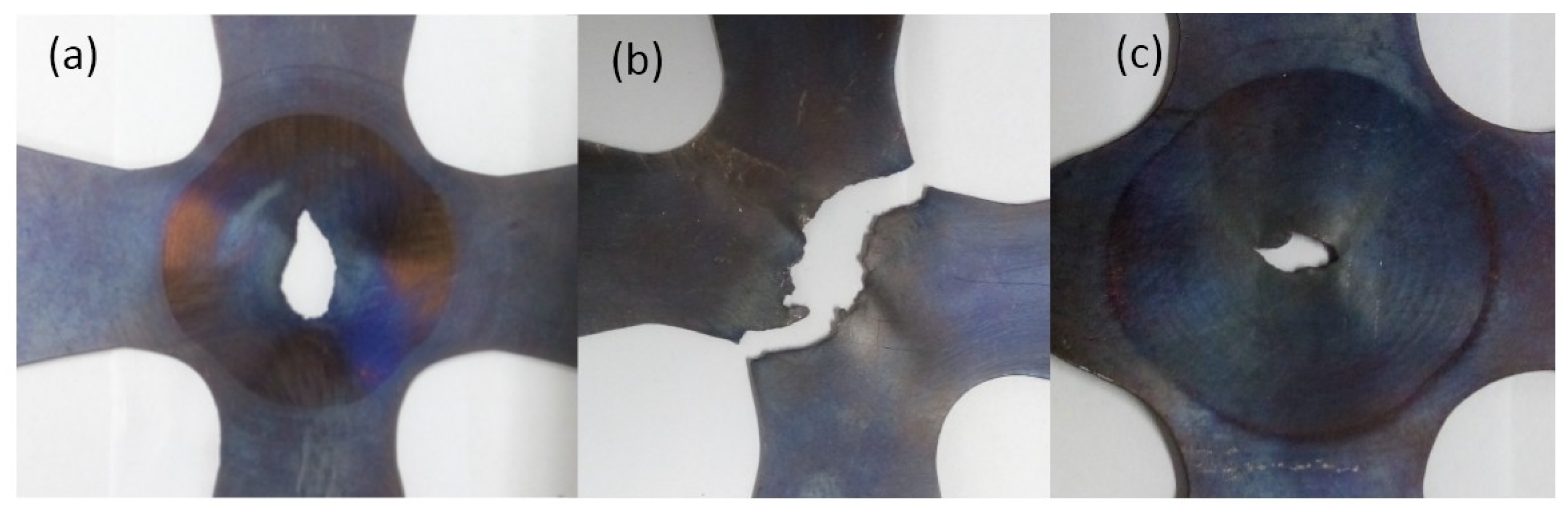
4.1. Experimental Details of the Biaxial Tensile Test

The biaxial tensile test of metal sheet is becoming increasing popular recently in sheet metal forming industries [26,27]. As in sheet metal forming operations, the material is often subjected to deformation in more than one plane or axis. So the mechanical properties obtained by uniaxial tensile test are inadequate for predicting the material’s deformation under states of biaxial stress [28]. Hannon et al. [28] reviewed several types of biaxial tensile test machines developed by Makinde [29], Kuwabara [30], etc. However, in the current literatures, few biaxial tensile test equipment could handle the testing procedure of metal sheet at relative high temperatures (e.g., above 400 °C). Lang et al. [31] developed a servo-hydraulic 100-kN hot biaxial tensile test machine in 2015 (as shown in Figure 9) on which the biaxial test was performed. The maximum displacement of each axis is 100 mm with the displacement control accuracy of each axis higher than 0.02 mm. The heating furnace is placed at the center of the pedestal, it could generate and maintain a constant temperature from room temperature to 800 °C.
The design of biaxial test specimen is a challenging task, many cruciform specimens have been proposed to obtain the biaxial stress state of the test material at the center section of the specimen and to avoid stress concentrations outside the gauge area [28,32], but up to now, there is no standard specimen geometry in the literature [33], which makes it difficult to compare test results from different research institutes. In this study, a special designed thickness-tapered cruciform specimen is adopted in the test as illustrated in Figure 10. To concentrate strains in the central zone, the central region of the specimen is machined to make the upper surface of the test piece be part of a sphere with the radius of around 250.4 mm. The minimum thickness in the center is 0.2 mm, which could ensure that the final failure occurs in this section. In order to avoid strain localization at the junction of two arms, the rounding radius at the intersection of two arms is made 12 mm. The hot biaxial tensile test was performed at the same condition with the hot uniaxial tensile test, i.e., at 500 °C and at different strain rates (0.1 s−1, 0.02 s−1 and 0.005 s−1). It should be noted that the accurate strain value of the test specimen is difficult to be acquired, so the relatively consistent strain rate is achieved with the application of finite element analysis which will be discussed in Section 4.2. The result of the test is plotted in Figure 11. We can observe that the material presents a rate-dependent property as well at equi-biaxial tensile condition. The fractured specimen after the test is shown in Figure 12. It can be discovered that the special designed specimen with a reduced center section could guarantee that the maximum deformation occurs in the center.

4.2. FE Analysis of Biaxial Tensile Test

The accurate stress and strain of the special designed cruciform specimen is difficult to be calculated. So we adopted FE analysis to evaluate the hardening curves at biaxial stress state. The isotropic elastic-plastic numerical model is established by using the commercial FEA program ABAQUS as shown in Figure 13. The cruciform specimen is modeled with 8-node linear reduced integration element (C3D8R). Due to the symmetrical properties of the specimen, only one-quarter of the model is modeled (Figure 13). Figure 14 shows the von Mises equivalent stress distribution of the specimen when the displacement of each axis reach 3.0 mm. The simulation result also demonstrates that the central section of the specimen experiences the maximum deformation. In addition, with the help of FEA, the relationship between the grip displacement and maximum strain could be established. Using Equation (3), the relatively accurate strain rate could be achieved by controlling the grip speed.
ε ¯ ˙ = d ε / d t = d ε / d U · d U / d t = d ε / d U · v
where U is the grip displacement and v is the grip speed.

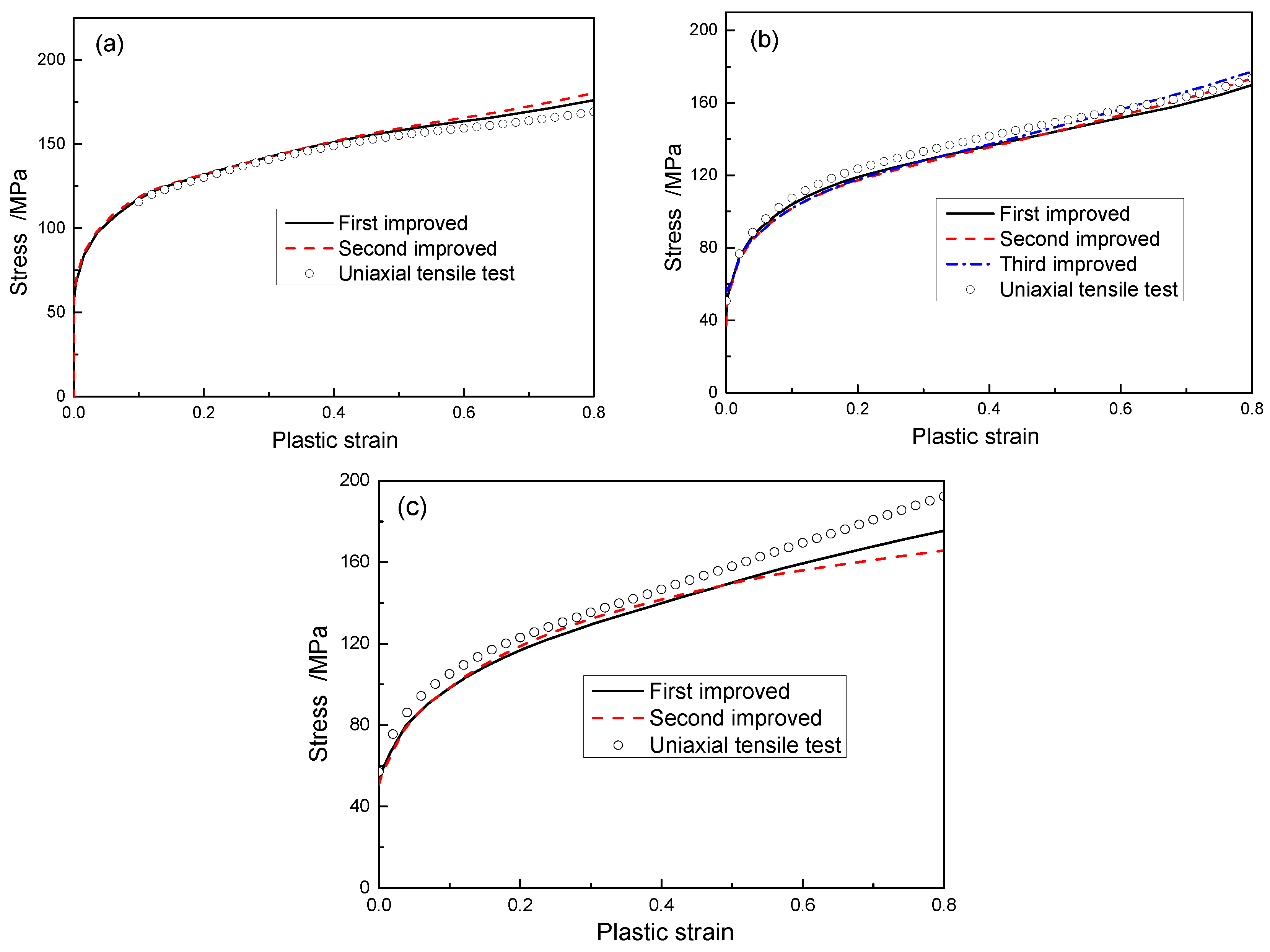
4.3. Validation of the Inverse Model

Figure 15 shows the improved stress-plastic strain curves of the investigated material in the biaxial tensile test by the inverse modeling method as described in Section 2.2. The hardening curves of the uniaxial tensile test obtained by the inverse method at corresponding conditions are also plotted in the figure. In order to reduce the iteration steps, the post-necking hardening curve calculated in Section 3 is regarded as the initial guess in the iterative step. We can see from the figure that the iterative process converges to a certain value after two or three steps. At strain rate of 0.1 s−1 and 0.02 s−1, the flow stress of the biaxial test obtained by the inverse method is close to the uniaxial test result. It should be noted that the achieved minimum relative mean square errors Φ are 0.97%, 1.01% and 2.94% for strain rate of 0.1 s−1, 0.02 s−1 and 0.005 s−1 respectively, which is much larger than the optimized values calculated in Section 3. In other words, the proposed inverse modeling method is able to obtain the hardening curve using complex specimens such as the special designed cruciform test piece, but the precision is not very high.

5. Conclusions

The post-necking hardening behaviors of uniaxial tensile test and biaxial tensile test are determined by using the inverse modeling method. The following conclusions can be derived from this study:
(1). By using the proposed inverse method, the internal relation between the plastic strain and elongation of the uniaxial tensile test could be automatically obtained without the application of any non-contact optical measurement.
(2). If the stress-strain curve in the inverse modeling method is represented by simple classical hardening laws, the convergence condition of the inverse iteration procedure cannot be finally satisfied.
(3). The extrapolated hardening curve using phenomenological constitutive models greatly depends on the model that is selected and it will be in poor accuracy for predicting the post-necking hardening curve of metal sheet.
(4). The proposed inverse modeling method could be used to obtain the hardening curve of metal sheet using complex specimens such as the special designed cruciform test piece, but the calculation accuracy is not very high.

Author Contributions

H.M. and L.L. conceived and designed the experiments; H.M. performed the experiments; H.M. and K.L. analyzed the data; H.M. wrote the paper; L.L. and X.Y. contributed to the revision of the paper.

Funding

This research received no external funding.

Conflicts of Interest

The authors declare no conflict of interest.

References

  1. Huang, C.Q.; Liu, L.L. Application of the Constitutive Model in Finite Element Simulation: Predicting the Flow Behavior for 5754 Aluminum Alloy during Hot Working. Metals 2017, 7, 1–12. [Google Scholar]
  2. Kajberg, J.; Lindkvist, G. Characterisation of materials subjected to large strains by inverse modelling based on in-plane displacement fields. Int. J. Solids Struct. 2004, 41, 3439–3459. [Google Scholar] [CrossRef]
  3. Coppieters, S.; Kuwabara, T. Identification of Post-Necking Hardening Phenomena in Ductile Sheet Metal. Exp. Mech. 2014, 54, 1355–1371. [Google Scholar] [CrossRef]
  4. Grajcar, A.; Kozlowska, A.; Grzegorczyk, B. Strain Hardening Behavior and Microstructure Evolution of High-Manganese Steel Subjected to Interrupted Tensile Tests. Metals 2018, 8, 1–12. [Google Scholar] [CrossRef]
  5. Enami, K. The effects of compressive and tensile prestrain on ductile fracture initiation in steels. Eng. Fract. Mech. 2005, 72, 1089–1105. [Google Scholar] [CrossRef]
  6. Coppieters, S.; Cooreman, S.; Sol, H.; Houtte, P.V.; Debruyne, D. Identification of the post-necking hardening behaviour of sheet metal by comparison of the internal and external work in the necking zone. J. Mater. Process. Technol. 2011, 211, 545–552. [Google Scholar] [CrossRef]
  7. Bridgman, P.W. Studies in Large Plastic Flow and Fracture; McGraw Hill: New York, NY, USA, 1952; pp. 15–20. [Google Scholar]
  8. Ling, Y. Uniaxial true stress-strain after necking. AMP. J. Tech. 1996, 5, 37–48. [Google Scholar]
  9. Zhang, Z.L.; Hauge, M.; Ødegård, J.; Thaulow, C. Determining material true stress–strain curve from tensile specimens with rectangular cross-section. Int. J. Solids Struct. 1999, 36, 3497–3516. [Google Scholar] [CrossRef]
  10. Mirone, G. A new model for the elastoplastic characterization and the stress–strain determination on the necking section of a tensile specimen. Int. J. Solids Struct. 2004, 41, 3545–3564. [Google Scholar] [CrossRef]
  11. Cabezas, E.E.; Celentano, D.J. Experimental and numerical analysis of the tensile test using sheet specimens. Finite Elem. Anal. Des. 2004, 40, 555–575. [Google Scholar] [CrossRef]
  12. Tong, W.; Tao, H.; Zhang, N.; Jiang, X.Q.; Manuel, P.M.; Louis, G.H.; Xiaohong, Q.G. Deformation and Fracture of Miniature Tensile Bars with Resistance-Spot-Weld Microstructures. Metall. Mater. Trans. A 2005, 36, 2651–2669. [Google Scholar] [CrossRef]
  13. Yang, S.Y.; Tong, W.A. Finite Element Analysis of a Tapered Flat Sheet Tensile Specimen. Exp. Mech. 2009, 49, 317–330. [Google Scholar] [CrossRef]
  14. Scheider, I.; Cornec, A.; Brocks, W. Procedure for the Determination of True Stress-Strain Curves from Tensile Tests with Rectangular Cross-Section Specimens. J. Eng. Mater. Technol. 2004, 126, 70–76. [Google Scholar] [CrossRef]
  15. Kamaya, M.; Kawakubo, M. A procedure for determining the true stress–strain curve over a large range of strains using digital image correlation and finite element analysis. Mech. Mater. 2011, 43, 243–253. [Google Scholar] [CrossRef]
  16. Faurholdt, T.G. Inverse modelling of constitutive parameters for elastoplastic problems. J. Strain Anal. Eng. Des. 2000, 35, 471–478. [Google Scholar] [CrossRef]
  17. Koc, P.; Štok, B. Computer-aided identification of the yield curve of a sheet metal after onset of necking. Comput. Mater. Sci. 2004, 31, 155–168. [Google Scholar] [CrossRef]
  18. Rossi, M.; Pierron, F. Identification of plastic constitutive parameters at large deformations from three dimensional displacement fields. Comput. Mech. 2012, 49, 53–71. [Google Scholar] [CrossRef]
  19. Kim, J.H.; Serpantié, A.; Barlat, F.; Pierron, F.; Lee, M.G. Characterization of the post-necking strain hardening behavior using the virtual fields method. Int. J. Solids Struct. 2013, 50, 3829–3842. [Google Scholar] [CrossRef]
  20. Joun, M.S.; Eom, J.G.; Min, C.L. A new method for acquiring true stress–strain curves over a large range of strains using a tensile test and finite element method. Mech. Mater. 2008, 40, 586–593. [Google Scholar] [CrossRef]
  21. Joun, M.; Choi, I.; Eom, J.; Lee, M. Finite element analysis of tensile testing with emphasis on necking. Comput. Mater. Sci. 2007, 41, 63–69. [Google Scholar] [CrossRef]
  22. Coppieters, S.; Ichikawa, K.; Kuwabara, T. Identification of Strain Hardening Phenomena in Sheet Metal at Large Plastic Strains. Procedia Eng. 2014, 81, 1288–1293. [Google Scholar] [CrossRef]
  23. Kuwabara, T.; Sugawara, F. Multiaxial tube expansion test method for measurement of sheet metal deformation behavior under biaxial tension for a large strain range. Int. J. Plast. 2013, 45, 103–118. [Google Scholar] [CrossRef]
  24. Hu, M.; Dong, L.M.; Zhang, Z.Q.; Lei, X.F.; Yang, R.; Sha, Y.H. Correction of Flow Curves and Constitutive Modelling of a Ti-6Al-4V Alloy. Metals 2018, 8, 1–15. [Google Scholar] [CrossRef]
  25. Tsao, L.C.; Wu, H.Y.; Leong, J.C.; Fang, C.J. Flow stress behavior of commercial pure titanium sheet during warm tensile deformation. Mater. Des. 2012, 34, 179–184. [Google Scholar] [CrossRef]
  26. Shiratori, E.; Ikegami, K. A new biaxial tensile testing machine with flat specimen. Bull. Tokyo Inst. Technol. 1967, 82, 105–118. [Google Scholar]
  27. Kulawinski, D.; Ackermann, S.; Seupel, A.; Lippmann, T.; Henkel, S.; Kuna, M.; Weidner, A.; Biermann, H. Deformation and strain hardening behavior of powder metallurgical TRIP steel under quasi-static biaxial-planar loading. Mater. Sci. Eng. A 2015, 642, 317–329. [Google Scholar] [CrossRef]
  28. Hannon, A.; Tiernan, P. A review of planar biaxial tensile test systems for sheet metal. J. Mater. Process. Technol. 2008, 198, 1–13. [Google Scholar] [CrossRef]
  29. Makinde, A.; Thibodeau, L.; Neale, K.W.; Lefebvre, D. Design of a biaxial extensometer for measuring strains in cruciform specimens. Exp. Mech. 1992, 32, 132–137. [Google Scholar] [CrossRef]
  30. Kuwabara, T.; Ikeda, S.; Kuroda, K. Measurement and analysis of differential work hardening in cold-rolled steel sheet under biaxial tension. J. Mater. Process. Technol. 1998, 80–81, 517–523. [Google Scholar] [CrossRef]
  31. Xiao, R.; Li, X.X.; Lang, L.H.; Chen, Y.K.; Yang, Y.F. Biaxial tensile testing of cruciform slim superalloy at elevated temperatures. Mater. Des. 2016, 94, 286–294. [Google Scholar] [CrossRef]
  32. Welsh, J.S.; Adams, D.F. An experimental investigation of the biaxial strength of IM6/3501-6 carbon/epoxy cross-ply laminates using cruciform specimens. Compos. Part A 2002, 33, 829–839. [Google Scholar] [CrossRef]
  33. Leotoing, L.; Guines, D. Investigations of the effect of strain path changes on forming limit curves using an in-plane biaxial tensile test. Int. J. Mech. Sci. 2015, 99, 21–28. [Google Scholar] [CrossRef] [Green Version]
Figure 1. (a) Geometry of tensile specimen (unit: mm), (b) specimen after fracture.
Metals 08 01044 g001
Figure 2. Traction force versus displacement in tensile test.
Metals 08 01044 g002
Figure 3. Schematic diagram of the inverse method.
Metals 08 01044 g003
Figure 4. Improved stress-plastic strain curves by inverse method at different strain rates (a) 0.005 s−1 (b) 0.02 s−1 (c) 0.1 s−1.
Metals 08 01044 g004
Figure 5. Relationship between elongation and plastic strain at different strain rates (a) 0.005 s−1 (b) 0.02 s−1 (c) 0.1 s−1.
Metals 08 01044 g005
Figure 6. Relative mean square error Φ versus iterative step at different strain rates.
Metals 08 01044 g006
Figure 7. The entire stress-plastic strain curve fitted by classical hardening laws.
Metals 08 01044 g007
Figure 8. Extrapolation of three classical hardening laws.
Metals 08 01044 g008
Figure 9. Biaxial tensile test machine.
Metals 08 01044 g009
Figure 10. Specimen geometry of the biaxial tensile (unit: mm), where A-A is the cross section.
Metals 08 01044 g010
Figure 11. Specimen geometry of the biaxial tensile (unit: mm).
Metals 08 01044 g011
Figure 12. Fractured specimen after biaxial test (a) 0.1 s−1 (b) 0.02 s−1 (c) 0.005 s−1.
Metals 08 01044 g012
Figure 13. FE analysis of cruciform specimen.
Metals 08 01044 g013
Figure 14. FE simulation result of cruciform specimen.
Metals 08 01044 g014
Figure 15. Improved stress-plastic strain curves and uniaxial test data at different strain rates. (a) 0.1 s−1 (b) 0.02 s−1(c) 0.005 s−1.
Metals 08 01044 g015
Table 1. Other phenomenological constitutive models.
ModelExpression
Swift σ = K ( p + ε 0 ) n
Voce σ = σ s ( σ s σ 1 ) e n p
Ludwik σ = σ 0 + K p n
where σ is the Cauchy stress, p is the plastic strain and the others are the fitting parameters.
Table 2. Parameter values for each constitutive models.
ModelSwiftVoceLudwik
Parameter K = 202.93 σ s = 230.84 σ 0 = 55.620
ε 0 = 0.03435 σ l = 66.31 K = 152.73
n = 0.3586 n = 1.812 n = 0.5318
Table 3. Parameter values for each constitutive models.
ModelSwiftVoceLudwik
Parameter K = 178.75 σ s = 121.25 σ 0 = 53.437
ε 0 = 0.00731 σ l = 57.37 K = 169.21
n = 0.2375 n = 15.000 n = 0.5186

