The Simulation of Extremely Low Cycle Fatigue Fracture Behavior for Pipeline Steel (X70) Based on Continuum Damage Model

Abstract

Natural gas transmission pipelines installed in seismic and permafrost regions are vulnerable to cyclic loads with a large strain amplitude. Under these conditions, the pipe may fail in extremely low cycles, a situation which is also known as extremely low cycle fatigue (ELCF) failure. The fracture mechanism of ELCF shows significant difference to that of low cycle fatigue, and the ELCF life usually deviates from the Coffin–Manson law. Thus, it is essential to develop an effective model to predict ELCF failure of the pipeline. In this study, a series of ELCF tests is performed on pipeline steel (X70). A damage coupled mixed hardening model is developed to simulate the fracture behaviors. Continuum damage law under monotonic load is extended to cyclic load by introducing the effective equivalent plastic strain. By assuming the cyclic softening is induced by the damage accumulation, the damage parameters are fitted directly from the peak stress in each cycle. Then, the model is input into commercial software ABAQUS with a user material subroutine to simulate the fracture behaviors of these specimens. The simulation results show good agreements with the test results both under cyclic and monotonic load, which verifies the reliability of the model.

1. Introduction

Pipeline transportation has been widely used in the oil and gas industry; it is one of the safest modes of transportation and has failure rates much lower than railroad or highway transportation [1]. However, failures do occur, and the fracture failure of pipelines may have catastrophic consequences. In order to conduct fracture failure analysis of pipelines effectively, it is necessary to identify the fracture modes of the pipeline material that may occur during a pipeline’s service [2,3,4]. Fracture modes of pipeline steel can be commonly classified into several categories, including ductile fracture, brittle fracture and fatigue fracture [5,6,7,8,9,10,11]. Pipeline steel is generally required to have high plasticity and toughness. Under large strain loads, pipeline steel undergoes ductile fracture, accompanied by the nucleation, growth and coalescence of void at the microscopic level [8,9,12]. At low temperatures, brittle fracture of the pipeline steel may occur due to a decrease in toughness [10,13]. Fatigue fracture is also a common failure mode of pipeline steel which occurs under cyclic load [5,6,14]. According to the fatigue cycles, fatigue fracture can be further divided into low cycle fatigue fracture (LCF, N_f < 10,000) and high cycle fatigue fracture (HCF, N_f > 10,000). LCF fracture is usually associated with localized plastic deformation [7,11]. The ductile fracture, brittle fracture and fatigue fracture of pipeline steel have been intensively investigated.

However, with the exploitation of oil and gas expanding into seismic and permafrost regions, pipelines are more vulnerable to cyclic loads with a large strain amplitude [15,16,17]. Under such conditions, pipes may undergo large plastic deformation and fail in extremely low cycles (N_f < 100), which is also called extremely low cycle fatigue (ELCF) [18,19,20,21]. The fracture behavior of the ELCF shows significant difference to that of general LCF. Under a large strain cyclic load, the material will undergo obvious strain hardening or softening phenomenon. In addition, compared with the generation and expansion of micro-cracks under fatigue load, the fracture mechanism of the ELCF is more similar to the ductile fracture mechanism under monotonic load [22,23]. On the fracture surface of the ELCF, the nucleation and growth of void can be clearly observed [18]. Therefore, the ELCF life usually deviates from the Coffin–Manson law, which is widely used to predict LCF life [15]. It is essential to develop an effective model to predict the ELCF failure of pipeline according to its fracture mechanism.

Recently, a series of ductile fracture models have been proposed in the literature [24,25,26,27,28]. These models can be mainly divided into two categories: damage uncoupled and damage coupled fracture models [29,30]. The uncoupled model ignores the degradation of macroscopic mechanical properties such as strength and stiffness due to damage accumulation [31,32]. These models can be further classified as empirical and physically based models [31]. Empirical models are developed based on experimental observations or theoretical analyses. The first empirical ductile fracture model was developed by using the plastic work as a damage indicator [29]. Since then, numerous empirical models have been developed based on the consideration of various factors causing ductile fracture [31,33]. Physically based models for ductile fracture are developed according to the mechanisms of void nucleation, void growth and void coalescence. Several micro-mechanism-inspired uncoupled models were proposed to predict the initiation of fracture under various stress states [34,35].

The damage coupled model integrates the constitutive properties of materials, and it can predict the deterioration of mechanical properties caused by damage accumulation [29,30]. The Gurson–Tvergaard–Needleman (GTN) model is one of the well-known damage coupled models, and was developed on the basis of a series of researchers’ achievements [36,37,38]. Firstly, Gurson proposed the initial porous plasticity model [39]. Then, the void nucleation effect, void interaction effect and void coalescence mechanism were introduced to establish the final GTN model [40]. In addition to the GTN model, Lemaitre [41] proposed another coupled ductile fracture model based on the theories of continuum damage mechanics and thermodynamics, namely the continuum damage mechanics (CDM) model. Rather than describing the changes in micro-void, the CDM model pays more attention to the process of damage evolution and the influence of damage on the macroscopic mechanical properties [25,28]. Compared to the uncoupled model, the damage coupled model can reflect the actual process of plastic deformation and damage evolution of materials more accurately [42]. However, due to the integration of material constitutive relations, these models often contain more parameters. The determination of these parameters is usually difficult work [29,30].

Several ELCF models have been proposed according to the empirical or physically based ductile fracture models [20,43,44,45]. The Mohr–Coulomb ductile fracture model was extended to predict ELCF fracture by introducing two weight functions [46]. By assuming the rate of void expansion is equal to the rate of void contraction, a cyclic void growth model (CVGM) and a degradation significant plastic strain (DSPS) model were proposed based on the void growth (VGM) model and the stress modified critical strain (SMCS) model, respectively [47]. Smith proposed the stress weighted ductile fracture (SWDF) model to modify the CVGM model under moderate and low stress triaxiality [48]. However, most of the current work for predicting ELCF fracture behavior focuses on the damage uncoupled models [15,18]. The availability of damage coupled models for ELCF fracture is limited in the literature.

Thus, in this study, the CDM model under monotonic load is extended to cyclic load by introducing the effective equivalent plastic strain. Combined with a mixed hardening criterion, the damage coupled model is developed to simulate the ELCF fracture behavior of the pipeline steel (X70). By assuming the cyclic softening is induced by the damage accumulation, the damage parameters can be fitted directly from the test results, which solves the difficult problem of parameter determination in damage coupled models. Then, the model is input into commercial software ABAQUS with user material subroutine (VUMAT) to simulate the fracture behaviors. At the end, the fracture characteristics of the ELCF are analyzed according to the internal variables in VUMAT.

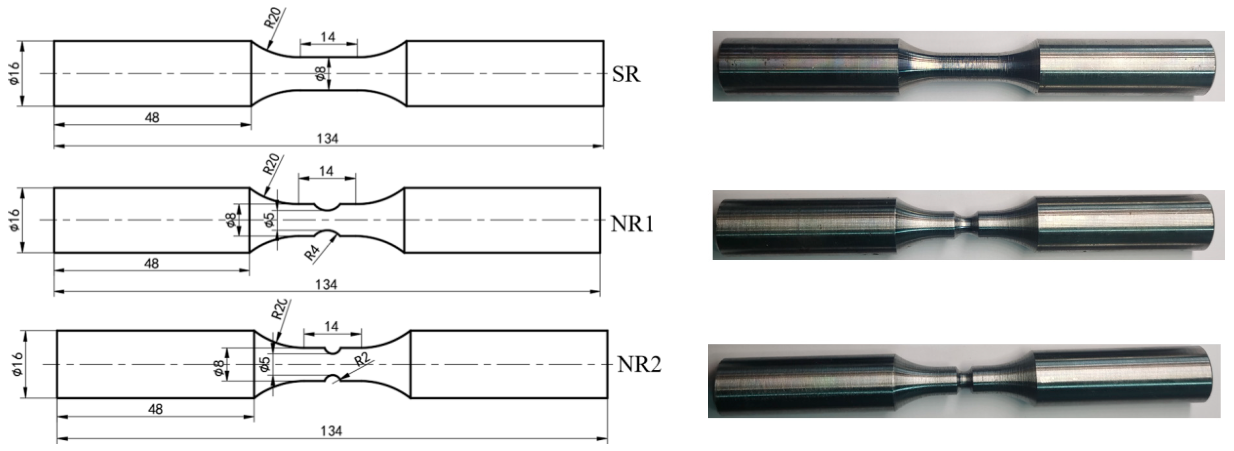
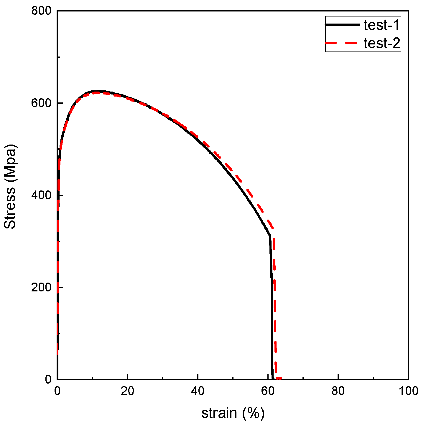
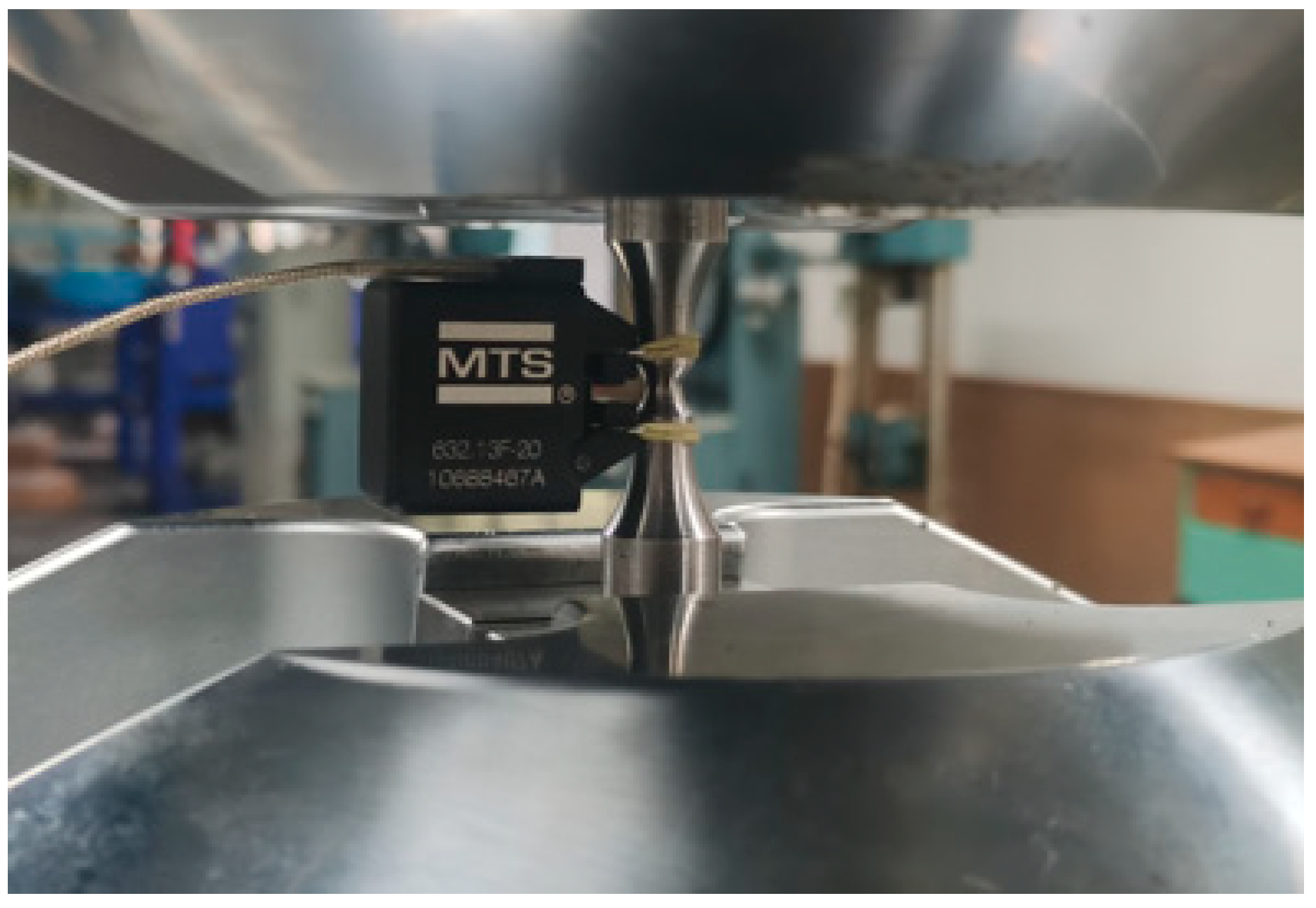
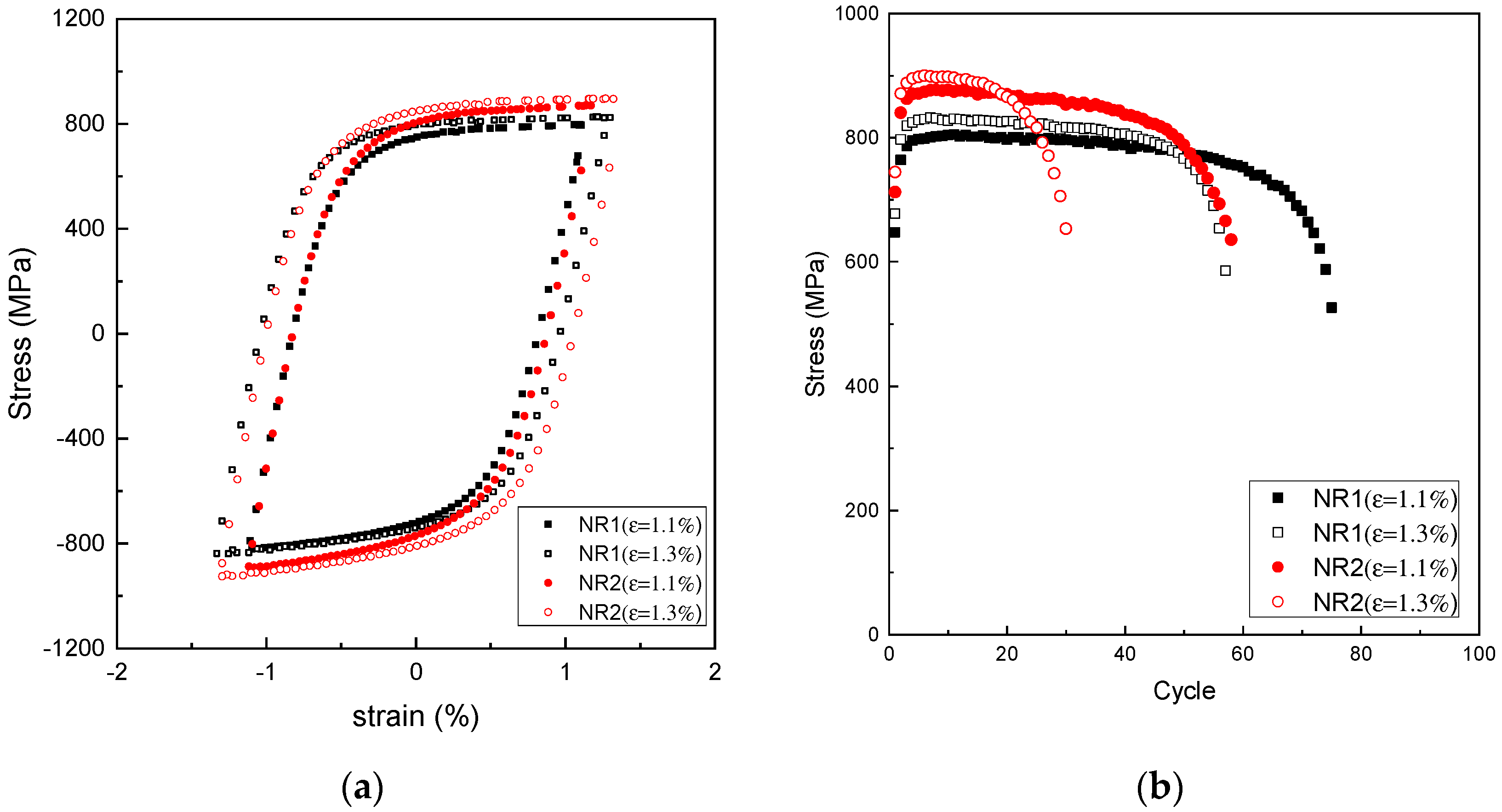
2. ELCF Tests

The pipeline steel (X70) used in this study was manufactured using the thermo-mechanical controlled process (TMCP) [17,49], and has a higher deformability compared to traditional X70 steel. A series of uniaxial monotonic and cyclic load tests were carried out on three types of specimens. Figure 1 shows the geometries and pictures of these specimens: smooth round (SR) and notched round (NR) specimens with two different notch radii (the notch radius were R = 2.0 and 4.0 mm). The tests were performed using a universal test machine (MTS Inc., Minneapolis, MN, USA) and conducted at room temperature. The monotonic tests were performed under displacement-controlled mode with a loading rate of 1 mm/min. Tensile properties obtained from SR specimens are shown in Figure 2. The yield strength and tensile strength are 472.1 MPa and 626.2 MPa, respectively. The uniform deformation section can reach up to 10%.

A series of uniaxial symmetrical strain cyclic tests were performed in triangular waveform under the strain-controlled mode to evaluate the ELCF properties. The loading conditions are listed in

Table 1. Load conditions and results of ELCF tests.

No.	Specimen Type	Strain Amplitude	Loading Frequency	Cycles
1	SR	1.5%	0.02 Hz	49
2	SR	1.9%	0.02 Hz	68
3	SR	2.3%	0.02 Hz	95
4	NR1	1.1%	0.02 Hz	75
5	NR1	1.3%	0.02 Hz	57
6	NR2	1.1%	0.02 Hz	58
7	NR2	1.3%	0.02 Hz	30

with a loading frequency of 0.02 Hz. Figure 3 shows the test setup and the measured specimen. An extensometer with a gauge length of 10 mm was attached to the specimen to accurately measure the average strain on the test segment. The test results for the SR and NR specimens are shown in Figure 4 and Figure 5, respectively. It can be seen from Figure 4b that the whole lifetime of the ELCF can be broken into 3 stages: (1) the initial stage, (2) the steady stage and (3) the failure stage. Cyclic hardening is observed in the initial stage, while cyclic softening occurs in the steady stage, which is considered to be related to the damage evaluation. In the failure stage, the stress decreases dramatically with the initiation and propagation of macroscopic cracking. The cyclic softening (damage evolution) stage accounts for over 80% of the total lifetime. The test life to final fracture is listed in Table 1. It can be seen that both the strain amplitude and stress triaxiality (notch radius) have a significant effect on the ELCF life. With the increase in strain amplitude and stress triaxiality (the decrease in notch radius), the ELCF life decrease significantly.

3. Damage Coupled Mixed Hardening Model

3.1. CDM Model for ELCF

Based on Lemaitre’s work [41], damage law under monotonic load can be expressed as:

$${\left(D-D_0\right)}^{\frac{1-\alpha }{\alpha }}dD=\frac{K^2}{2E{S}_0}f(\frac{{\sigma }_m}{{\sigma }_e})\frac{dp}{p}$$

(1)

$$f(\frac{{\sigma }_m}{{\sigma }_e})=\frac{2\left(1+\nu \right)}{3}+3(1-2\upsilon ){(\frac{{\sigma }_m}{{\sigma }_e})}^2$$

(2)

where E is the elastic modulus; K and S₀ are the material parameters; D is the damage parameter and dD is the increment of accumulated damage. D₀ corresponds to the materials with no defect. p is the accumulated equivalent plastic strain. σ_e, σ_m and v are the von mises stress, hydrostatic stress and Poisson’s ratio, respectively. The damage evolution law in Equation (1) can be analytically integrated between (D_cr and D₀) and (p_cr and p_th) for uniform deformation during which the triaxiality factor remains constant (σ_m/σ_e = 1/3).

$${\left(D_{cr}-D_0\right)}^{\frac{1}{\alpha }}=\frac{1}{\alpha }\frac{K^2}{2E{S}_0}\ln (\frac{p_{cr}}{p_{th}})$$

(3)

where p_th is the threshold strain for damage initiation and D_cr is the critical amount of damage at the critical plastic strain, p_cr. Setting D₀ to 0 and substituting Equation (3) into Equation (1) yields:

$$dD=\alpha {D_{cr}}^{\frac{1}{\alpha }}{D}^{\frac{\alpha -1}{\alpha }}f(\frac{{\sigma }_m}{{\sigma }_e})\frac{dp}{p\mathrm{l}\mathrm{n}(\frac{p_{cr}}{p_{th}})}$$

(4)

Damage has been assumed to accumulate only in the tensile stress state (σ_m/σ_e > 0) in related research work [18,50]. Thus, in this study, the effective equivalent plastic strain is introduced to extend the CDM model under monotonic load to cyclic load, which is defined as:

$$d{p}^{+}=\left\{\begin{array}{c}dp \frac{{\sigma }_m}{{\sigma }_e}>0 \\ 0 \frac{{\sigma }_m}{{\sigma }_e}\le 0\end{array}\right.$$

(5)

Correspondingly, the damage evolution equation can be written as:

$$dD=\alpha {D_{cr}}^{\frac{1}{\alpha }}{D}^{\frac{\alpha -1}{\alpha }}f(\frac{{\sigma }_m}{{\sigma }_e})\frac{d{p}^{+}}{p^{+}\mathrm{l}\mathrm{n}(\frac{p_{cr}}{p_{th}})}$$

(6)

Then, the damage for SR specimens can be derived as:

$$D=D_{cr}(\frac{\ln \left(\frac{p^{+}}{p_{th}}\right)}{\ln \left(\frac{p_{cr}}{p_{th}}\right)}{)}^{\alpha }$$

(7)

This formulation allows the calibration of damage parameters directly from ELCF tests results of SR specimens.

3.2. Damage Coupled Mixed Hardening Model

In the constitutive framework of CDM, the effective stress is defined as:

$$\tilde{\mathsf{\sigma }}=\frac{\mathsf{\sigma }}{(1-D)}$$

(8)

Correspondingly, damage can be coupled to mixed hardening model with von Mises yield criterion:

$${\mathit{F}}_{\mathit{y}}=\sqrt{\frac{3}{2}\left(\frac{\mathit{S}}{(1-D)}-\mathit{a}\right):\left(\frac{\mathit{S}}{(1-D)}-\mathit{a}\right)}-Y$$

(9)

where S, a and Y are the deviatoric stress tensor, back stress tensor and yield stress, respectively. Back stress tensor characterizes the yield surface center and evolves according to Chaboche’s nonlinear kinematic hardening rule:

$$\mathit{a}=\sum {\mathit{a}}^{\mathit{i}}, i=1,2,3$$

(10)

$$\mathit{d}{\mathit{a}}^{\mathit{i}}=\frac{2}{3}{C}^{i}d{\mathit{\epsilon }}^{\mathit{p}}-{\gamma }^i{\mathit{a}}^{\mathit{i}}dp$$

(11)

where aⁱ is the ith component of deviatoric back stress a, ε^p is the plastic strain tensor and Cⁱ, γⁱ are the material parameters.

The yield stress is considered to vary according to nonlinear isotropic hardening:

$$Y=Q_0+Q_a[1-\mathrm{e}\mathrm{x}\mathrm{p}(Q_{b}p)]$$

(12)

where Q₀, Q_a and Q_b are the material parameters.

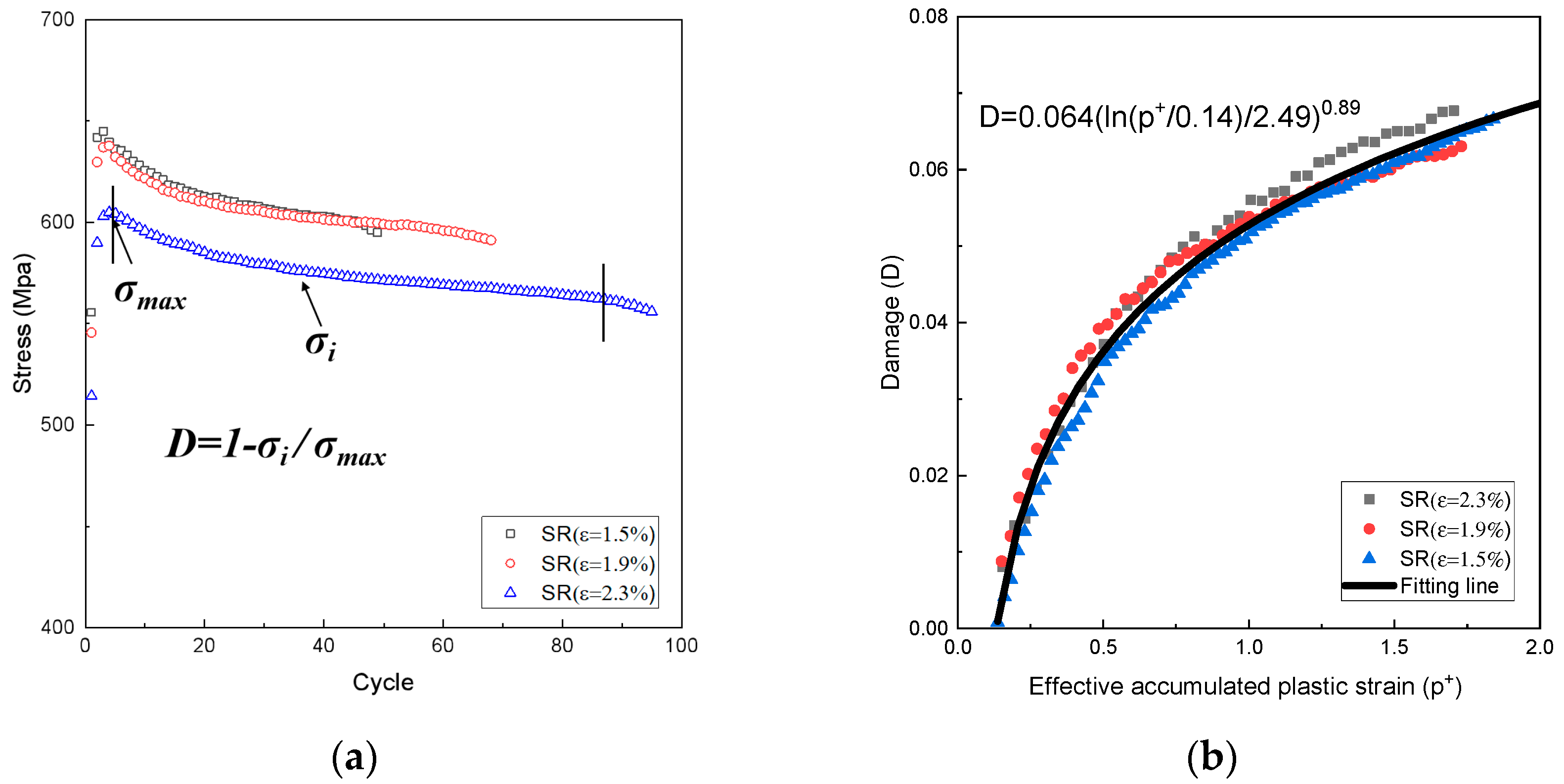
3.3. Calibration of Model Parameters

The hardening parameters are determined from a uniaxial strain-controlled stable hysteresis loop [50]. Assuming that in the stable hysteresis loop, γ¹ and γ² are large enough so that the back stresses a¹ and a² reach to their own extremum, while γ³ is relatively small so that the back stress a³ increases linearly through the entire loop. Then, C³ can be determined from the slope of the linear segment of hysteresis loop at high strain ranges. A large value of C¹/γ¹ is chosen to match the plastic modulus at yielding. The value of C²/γ² is adjusted to match the nonlinear portion of the stable hysteresis loop. Finally, the values of γ³, Q₀, Q_a and Q_b are determined according to the stress–strain curve in the first cycle. Values of the coefficients determined are tabulated in

Table 2. Parameters of damage coupled mixed hardening model.

Isotropic Hardening			Kinematic Hardening						Damage
Q0	Qa	Qb	C1	γ1	C2	γ2	C3	γ3	α	Dcr	pth	pcr
450	120	15	20,000	500	7000	200	1000	1	0.89	0.064	0.14	1.6

.

There are four damage evolution parameters (D_cr, α, p_cr and p_th) that should be calibrated. It is assumed that cyclic softening in the steady stage is caused by the accumulation of damage. Thus, the damage to SR specimens in each cycle can be quantified according to the decrease in peak stress in steady stage as shown in Figure 6a. Quantified damage (D) and effective accumulated equivalent plastic strain (p+) are obtained for SR specimens under cyclic load as shown in Figure 6b, which is fitted using Equation (7). Values of the damage parameters determined are tabulated in Table 2.

3.4. Numerical Algorithm to Solve Damage Coupled Mixed Hardening Model

This damage coupled mix hardening model is input into Abaqus user material subroutine VUMAT, which is globally following the explicit integration scheme, and which will give accurate material response at each time interval. The return mapping algorithm is employed locally and consists of two steps: elastic prediction and plastic correction. Assuming that all variables at time step t_n have been solved and the strain increment at time step t_n+1 is purely elastic, the trial stress at the time step t_n+1 can be obtained:

$${\mathit{\sigma }}_{\mathit{n}+1}^{\ast }=(1-D_n)\mathit{E}{:(\mathit{\epsilon }}_{\mathit{n}+1}-{\mathit{\epsilon }}_{\mathit{n}}^{\mathit{p}})$$

(13)

where $D_n$ is the damage at the time step t_n; E is the elastic stiffness tensor; ${\mathit{\epsilon }}_{\mathit{n}+1}$ is the strain tensor at the time step t_n+1 and ${\mathit{\epsilon }}_{\mathit{n}}^{\mathit{p}}$ is the plastic strain tensor at time step t_n. Similarly, in the following equations, the subscript n and n+1 indicate the variables at the time step t_n and t_n+1, respectively. In the case where:

$${\mathit{F}}_{\mathit{y}(\mathit{n}+1)}^{\ast }=\sqrt{\frac{3}{2}\left(\frac{{\mathit{S}}_{\mathit{n}+1}^{\ast }}{(1-D_n)}-{\mathit{a}}_{\mathit{n}}\right):\left(\frac{{\mathit{S}}_{\mathit{n}+1}^{\ast }}{(1-D_n)}-{\mathit{a}}_{\mathit{n}}\right)}-Y_n<0$$

(14)

$${\mathit{S}}_{\mathit{n}+1}^{\ast }={\mathit{\sigma }}_{\mathit{n}+1}^{\ast }-\frac{1}{3}Tr({\mathit{\sigma }}_{\mathit{n}+1}^{\ast })\mathit{I}$$

(15)

where ${\mathit{S}}_{\mathit{n}+1}^{\ast }$ is the trial deviatoric stress tensor the time step t_n+1, we have ${\mathit{\sigma }}_{\mathit{n}+1}={\mathit{\sigma }}_{\mathit{n}+1}^{\ast }$. Also, non-linear equation should be solved to obtain ${\mathsf{\Delta }\mathit{\epsilon }}_{\mathit{n}+1}^{\mathit{p}}.$ The deviatoric stress tensor at the time step t_n+1 is given by:

$${\mathit{S}}_{\mathit{n}+1}={\mathit{S}}_{\mathit{n}+1}^{\ast }-2G{\mathsf{\Delta }\mathit{\epsilon }}_{\mathit{n}+1}^{\mathit{p}}$$

(16)

Then, it can be obtained:

$${\mathit{S}}_{\mathit{n}+1}/(1-D_{n+1})-{\mathit{a}}_{\mathit{n}+1}=({\mathit{S}}_{\mathit{n}+1}^{\ast }-2G{\mathsf{\Delta }\mathit{\epsilon }}_{\mathit{n}+1}^{\mathit{p}})/(1-D_{n+1})-\sum _{i=1}^3{\mathit{a}}_{n+1}^i$$

(17)

According to Equations (10) and (11), we can have:

$${\mathit{a}}_{n+1}^i={\theta }_{n+1}^i({\mathit{a}}_n^i+\frac{2}{3}{C}^i{\mathsf{\Delta }\mathit{\epsilon }}_{\mathit{n}+1}^{\mathit{p}})$$

(18)

$${\theta }_{n+1}^i=\frac{1}{1+{\gamma }^i\Delta p_{n+1}}$$

(19)

According to the plastic flow criterion, it has:

$${\mathsf{\Delta }\mathit{\epsilon }}_{\mathit{n}+1}^{\mathit{p}}=\frac{3}{2}\mathsf{\Delta }{p}_{n+1}\frac{{\mathit{S}}_{\mathit{n}+1}/(1-D_{n+1})-{\mathit{a}}_{\mathit{n}+1}}{Y_{n+1}}$$

(20)

Combining Equation (20) with Equation (17), it can be derived as:

$${\mathit{S}}_{\mathit{n}+1}/(1-D_{n+1})-{\mathit{a}}_{\mathit{n}+1}=\frac{Y_{n+1}({\mathit{S}}_{\mathit{n}+1}^{*}/(1-D_{n+1})-\sum _{i=1}^3{{\theta }_{n+1}^i\mathit{a}}_n^i)}{Y_{n+1}+(3G+\sum _{i=1}^3{\theta }_{n+1}^i{C}^i)\Delta p_{n+1}}$$

(21)

With the yield criterion $F_{y(n+1)}=0$:

$$\Delta p_{n+1}=\frac{{\left[\frac{3}{2}({\mathit{S}}_{\mathit{n}+1}^{\ast }/(1-D_{n+1})-\sum _{i=1}^3{{\theta }_{n+1}^i\mathit{a}}_n^i):({\mathit{S}}_{\mathit{n}+1}^{\ast }/(1-D_{n+1})-\sum _{i=1}^3{{\theta }_{n+1}^i\mathit{a}}_n^i)\right]}^{\frac{1}{2}}-Y_{n+1}}{3G+\sum _{i=1}^3{\theta }_{n+1}^i{C}^i}$$

(22)

This is a nonlinear equation for $\Delta p_{n+1}$ which can be solved using Newton–Raphson iteration algorithm. Once $\Delta p_{n+1}$ is obtained, all the other variables can be updated accordingly.

4. Finite Element Analysis

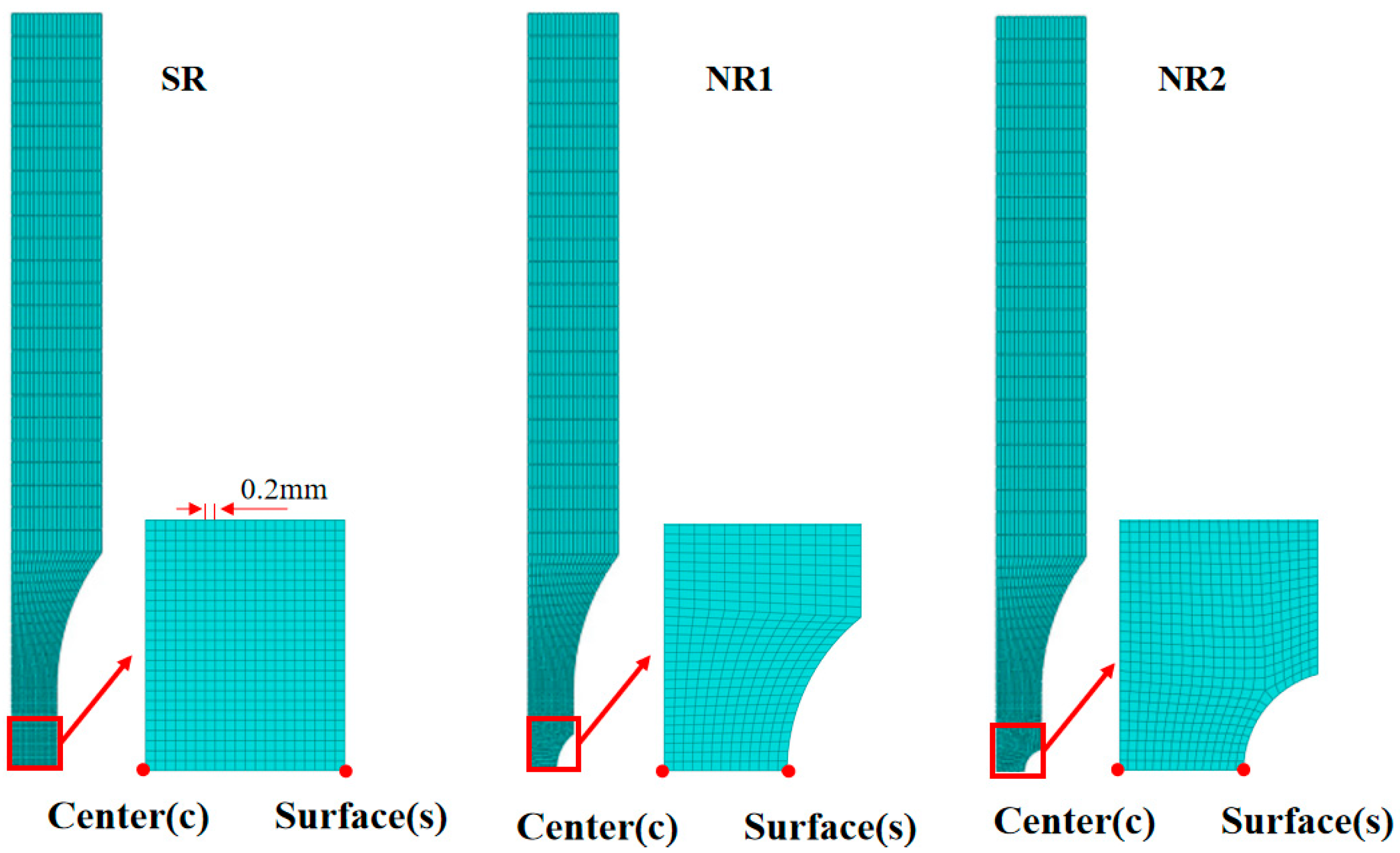
4.1. FEA Model

Axisymmetric FE models of SR and NR specimens are constructed in ABAQUS/Explicit 6.14. The dimensions are the same as those given in Figure 1. Reduced explicit linear axisymmetric elements (CAX4R) are applied in the models. As shown in Figure 7, the mesh size at the gauge section is selected to be as small as 0.2 mm for the convergence of mesh. This results in mesh of 1320 CAX4R elements and 1407 nodes, 1360 CAX4R elements and 1449 nodes and 1281 CAX4R elements and 1369 nodes, for the SR, NR1 and NR2 specimens. Boundary conditions follow those applied in the test. The material properties are defined with the Abaqus user material subroutine VUMAT, and the parameters calibrated according to the test results are used. To obtain the quasi-static state, semi-automatic mass scaling is used with a target time increment of 10⁻⁴ at the beginning of the step. The ratio of kinetic to internal energy is kept below 1%.

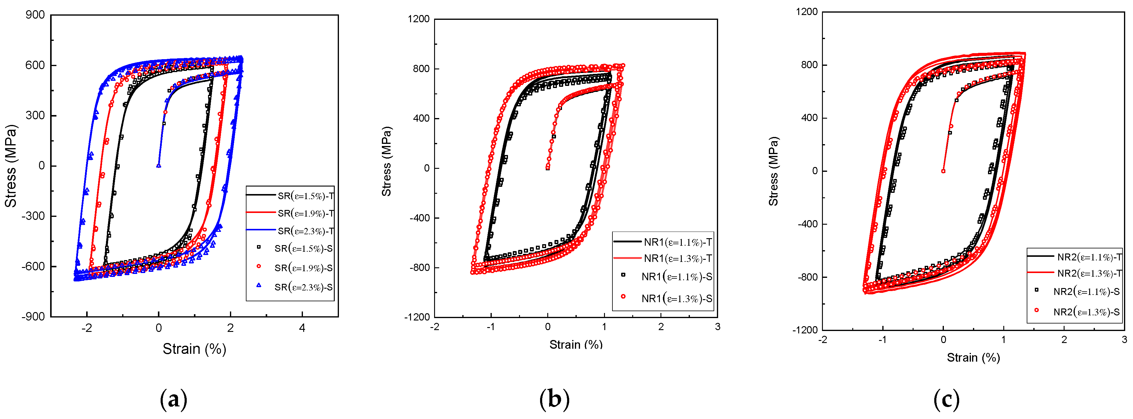
4.2. FEA Results

The comparison of engineering stress–strain curves in the first three cycles in the ELCF tests and the FEA are shown in Figure 8. In the case of the SR specimens, the FEA results show good agreements with those of the tests, while with the increase in stress triaxiality (the decrease in notch radius), slight deviations can be observed. Overall, the simulation precision is acceptable. The maximum deviation of predicted stress at the monitoring strain is around 6%.

Accumulated equivalent plastic strain contours for SR and NR specimens in various load cycles are shown in Figure 9. In the case of the SR specimen, plastic strain accumulates uniformly along the center to the surface. In the case of the NR specimens, plastic strain accumulates faster at the surface. However, what is interesting is that we can see that the crack initiates in the specimen center both for the SR specimen and NR specimens where there is slower accumulation rate of plastic strain. This phenomenon of cracking from the inside is consistent with the experimental observation [46].

To explain this phenomenon, damage contours for SR and NR specimens in various load cycles are shown in Figure 10. Similarly, damage accumulates uniformly along the center to the surface for the SR specimen. However, the NR specimens show a completely different pattern of damage accumulation. When the load cycles reach seven, damage accumulation initiates at the surface of the NR specimens. This can be attributed to the faster accumulation of plastic strain at the surface, as shown in Figure 9. After the accumulated plastic strain reaches the threshold strain for damage initiation, the accumulation of damage initiates. However, it can be clearly observed that the accumulation rate of damage at the specimen’s center is faster than that at the specimen surface for the NR specimens. When it closes to N_f/2 cycles, the damage at the specimen center of the NR1 specimen is almost equal to that at the specimen surface. However, for the NR2 specimen, the damage at the specimen surface is still dominant. When it closes to N_f cycles, the accumulation of damage in the specimen center is more than that at the specimen surface both for the NR1 and NR2 specimens. The crack initiates inside the specimens and propagates towards the outer radius.

As indicated in Equation (6), the accumulation rate of damage is affected not only by the accumulation rate of plastic strain, but also by the stress triaxiality. Thus, the stress triaxiality contours for the SR and NR specimens in various load cycles are shown in Figure 11. With the decrease in notch radius, the triaxiality shows an obvious increase. In the case of the SR specimen, the stress triaxiality is between 0.4 and 0.3 along the center to the surface at the initial loading. In the case of the NR1 specimen, the stress triaxiality is between 0.55 and 0.44 along the center to the surface at the initial loading. In the case of the NR2 specimen, the stress triaxiality is between 0.65 and 0.52 along the center to the surface at the initial loading. With the increase in load cycles, the stress triaxiality increases. When it closes to N_f cycles, the highest level the stress triaxiality reaches is 0.41, 0.72 and 0.79 for the SR, NR1 and NR2 specimens, respectively. The specimen center shows higher stress triaxiality both for the SR specimen and the NR specimens regardless of load cycles, which explains the phenomenon of cracking from inside. The damage and fracture behaviors of the ELCF simulated using the proposed model are similar to those seen in ductile fracture under monotonic load [28].

The quantitative comparison of damage accumulation is revealed in Figure 12. Figure 12a shows the evolution history of damage in specimen centers (point c, as noted in Figure 7) of the SR and NR specimens. It can be seen that both the strain amplitude and stress triaxiality (notch radius) have a significant effect on the accumulation of damage. Figure 12b compares the evolution history of damage at the specimen center and surface (point s, as noted in Figure 7). The faster accumulation of damage in the specimen center is verified. In addition, it can be seen that the damage to the NR2 specimen at point c and point s reach the critical value almost simultaneously. Thus, it can be assumed that the location for crack initiation is related to the notch shape. With the decrease in notch radius, the location for crack initiation may shift from the center to the surface.

As mentioned above, under cyclic loads with a large strain amplitude, the crack initiates in the specimen center. Thus, it is difficult in practice to accurately determine the life of crack initiation in tests. In this study, the specimens are loaded to final fracture, and the N_f is recorded. The macro-crack grows in several cycles before the final fracture of the specimen. The precise simulation of crack propagation in FEA is quite difficult work, as it is sensitive to the mesh size due to the stress concentration at the crack tip. However, a too small mesh size will greatly reduce computational efficiency. Since the lifetime for crack propagation is much shorter than that for crack initiation, accurate crack propagation simulation is not pursued in this study, which also has little effect on the prediction of final fracture life of these specimens. The lifetimes for the final fracture of the specimens in the FEA are obtained as shown in

Table 3. Comparison of ELCF life from test and FEA.

No.	Specimen Type	Strain Amplitude	Test Life (Cycle)	Predicted Life (Cycle)	Deviation
1	SR	1.5%	95	93	2.1%
2	SR	1.9%	68	69	−1.5%
3	SR	2.3%	49	54	−10.2%
4	NR1	1.1%	75	69	10.7%
5	NR1	1.3%	57	48	15.8%
6	NR2	1.1%	58	50	13.8%
7	NR2	1.3%	30	35	−16.7%

. Compared to the test life, the maximum deviation of predicted life is around 16%. Due to the discreteness and randomness of fatigue life itself, the developed model can be considered reasonable and promising. This model is also applied to predict the fracture of the SR and NR specimens under monotonic load. The predicted results are shown in Figure 13, which verifies that the damage parameters calibrated according to the ELCF test results are also suitable for monotonic load. In addition, in the simulation of the NR specimens under monotonic load, the accumulation of damage also begins at the specimen surface, while the crack initiation occurs in the specimen center.

4.3. Discussions

The determination of parameters in traditional damage coupling models is usually achieved by comparing the FE and experimental results repeatedly. For the models with various parameters, it is usually a difficult task. The developed model in this study provides an explicit expression between effective plastic strain and accumulated damage for the SR specimen, which allows us to fit the damage parameters directly from the test data. Furthermore, test data for the SR specimens under various loading condition (ε = 1.5%, 1.9% and 2.3%) can be used to fit the damage parameters simultaneously, which can improve the reliability of the developed model.

For thick-walled pipelines, the crack may propagate for a long time after the crack initiation. In that case, the crack propagation life should not be ignored for the final fracture failure prediction of pipelines. Theoretically, the proposed CDM based model can be used to predict both the crack initiation and propagation behaviors. The FEA results also show that the proposed model cannot only predict the lifetime but also the locations for crack initiation reasonably. However, the simulation of crack propagation may depend strongly on the mesh size. How to predict the whole life (crack initiation and propagation) of pipelines effectively while ensuring the computational efficiency is also an interesting topic.

5. Conclusions

In this study, a series of ELCF tests is performed on pipeline steel (X70), and a damage coupled mixed hardening model is developed to simulate the fracture behavior. The conclusions obtained are as following:

(1)

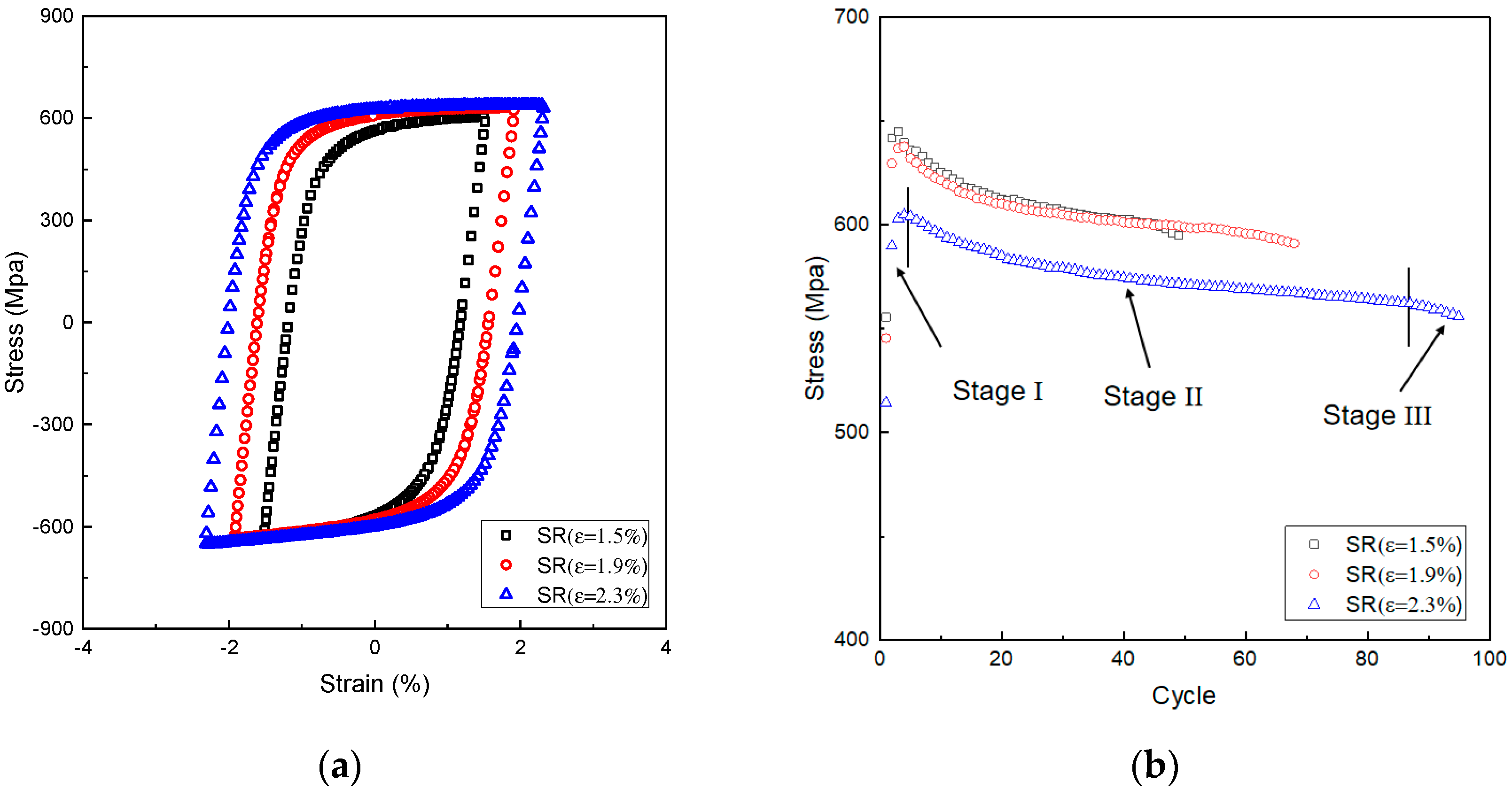
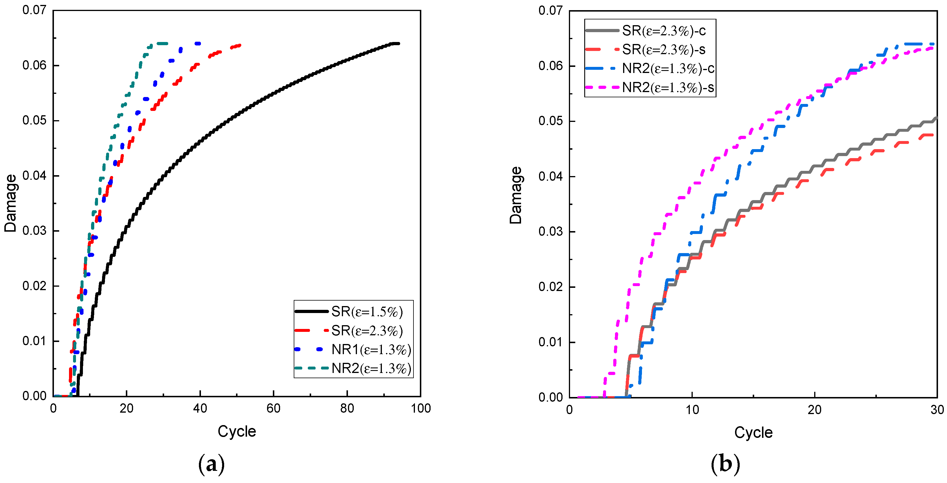
The lifetime of the ELCF for X70 can be broken into three stages: cyclic hardening, cyclic softening and the generation of macroscopic cracks. The cyclic softening (damage evolution) stage accounts for over 80% of the total lifetime. With the increase in strain amplitude and stress triaxiality, the ELCF life decreased significantly.

(2)

The continuum damage law under monotonic load is extended to cyclic load by introducing effective equivalent plastic strain. A damage coupled mixed hardening model is developed to predict the fracture behavior of the ELCF. This model provides an explicit expression between effective plastic strain and accumulated damage for the SR specimens, which makes the fitting of parameters simpler and more reliable.

(3)

The damage coupled mixed hardening model is numerically solved using Abaqus user material subroutine VUMAT. Compared to the test life, the maximum deviation of predicted life is around 16%, which verifies that the developed model is promising and reasonable.

(4)

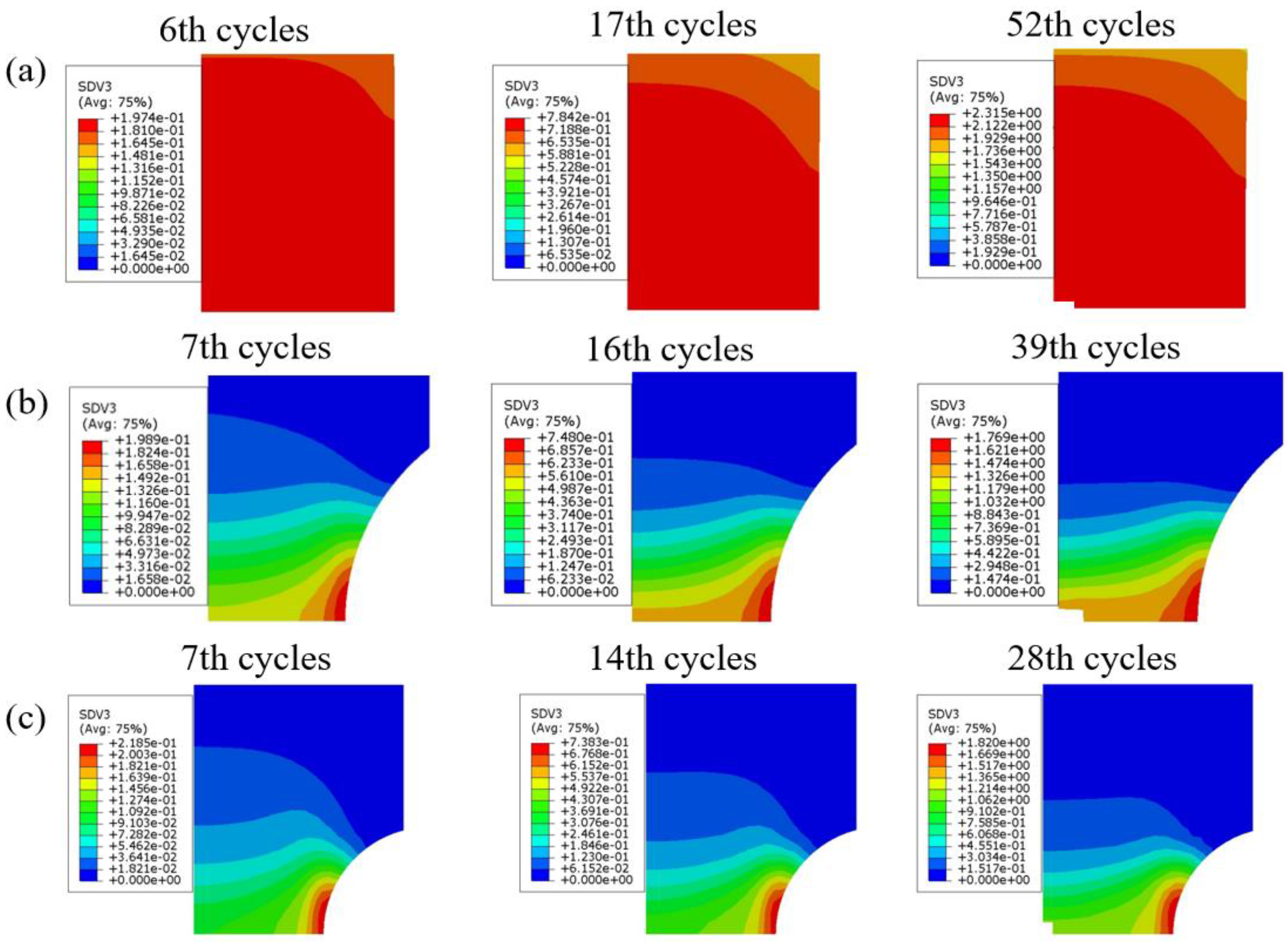
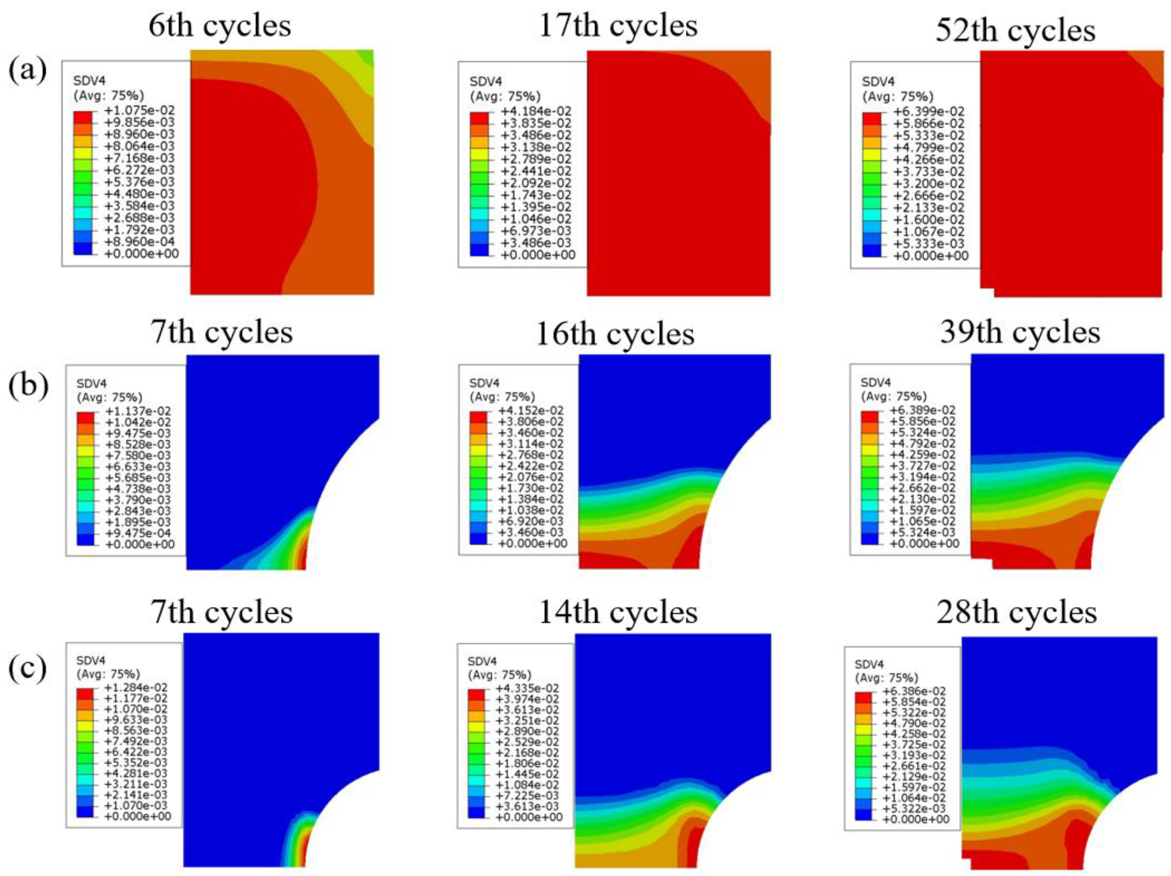
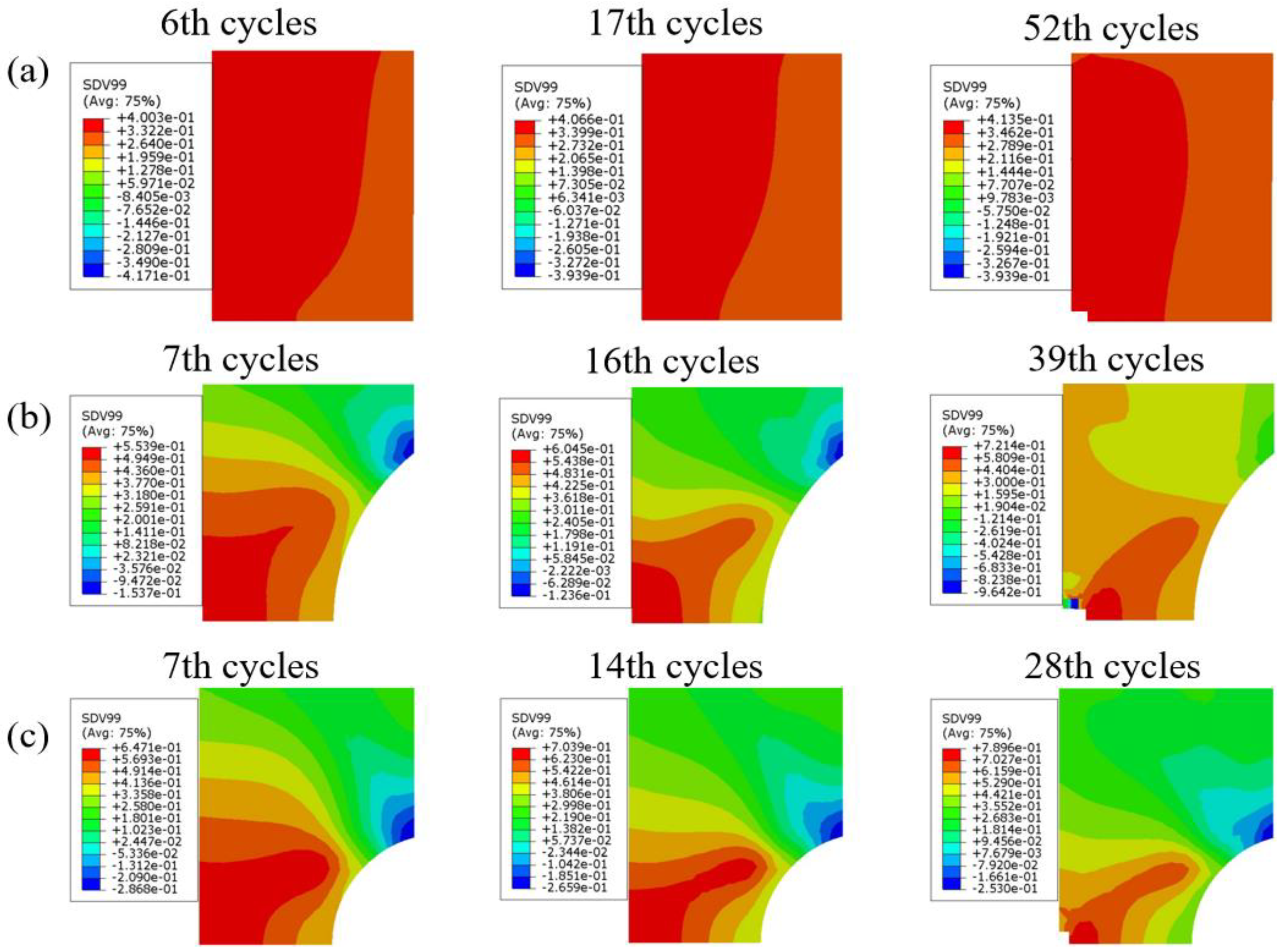
The FEA results show that the developed model cannot only predict the lifetime but also the locations of crack initiation reasonably. In the case of the NR specimens, though plastic strain accumulates faster in the surface of the specimen, the crack initiates from the specimen center due to the higher triaxiality. Such fracture behaviors are similar to those which occur in ductile fracture under monotonic load.

References

- Dey, P.K. Oil Pipelines. In Encyclopedia of Energy; Elsevier: Amsterdam, The Netherlands, 2004; pp. 673–690. [Google Scholar]
- Hu, X.Y.; Jia, J.H.; Wang, N.; Xia, X.M.; Wang, Z.D.; Tu, S.T. Design and Test of an Extensometer for Strainmonitoring of High Temperature Pipelines. J. Pressure Vessel. Technol. Trans. ASME 2012, 134, 044501. [Google Scholar] [CrossRef]
- Piątkowski, J.; Gajdzik, B.; Mesjasz, A. Assessment of Material Durability of Steam Pipelines Based on Statistical Analysis of Strength Properties—Selected Models. Energies 2020, 13, 3633. [Google Scholar] [CrossRef]
- Zaryankin, A.; Rogalev, N.; Rogalev, A.; Kocherova, A.; Strielkowski, W. Line Summary of Approaches for Improving Vibrational Reliability of Thermomechanical Equipment and Its Interconnecting Pipelines at Thermal Power Plant. Contemp. Eng. Sci. 2014, 7, 1793–1806. [Google Scholar] [CrossRef] [Green Version]
- Han, Y.; Zhong, S.; Peng, C.; Tian, L.; Sun, Y.; Zhao, L.; Xu, L. Fatigue Behavior of X65 Pipeline Steel Welded Joints Prepared by CMT/GMAW Backing Process. Int. J. Fatigue 2022, 164, 107156. [Google Scholar] [CrossRef]
- Faucon, L.E.; Boot, T.; Riemslag, T.; Scott, S.P.; Liu, P.; Popovich, V. Hydrogen-Accelerated Fatigue of API X60 Pipeline Steel and Its Weld. Metals 2023, 13, 563. [Google Scholar] [CrossRef]
- Song, Z.H.; Chen, N.Z. A Modified Cyclic Cohesive Zone Model for Low-Cycle Fatigue Crack Initiation Prediction for Subsea Pipelines under Mode I Loading. Ocean. Eng. 2023, 276, 114200. [Google Scholar] [CrossRef]
- Shen, F.; Münstermann, S.; Lian, J. Investigation on the Ductile Fracture of High-Strength Pipeline Steels Using a Partial Anisotropic Damage Mechanics Model. Eng. Fract. Mech. 2020, 227, 106900. [Google Scholar] [CrossRef]
- Paermentier, B.; Cooreman, S.; Verleysen, P.; Chandran, S.; Coppieters, S.; Talemi, R. A Dynamic Tensile Tear Test Methodology to Characterise Dynamic Fracture Behaviour of Modern High-Grade Pipeline Steels. Eng. Fract. Mech. 2022, 272, 108687. [Google Scholar] [CrossRef]
- Shen, F.; Pan, B.; Wang, S.; Lian, J.; Münstermann, S. Influence of Stress States on Cleavage Fracture in X70 Pipeline Steels. J. Pipeline Sci. Eng. 2022, 2, 100072. [Google Scholar] [CrossRef]
- Vishnuvardhan, S.; Murthy, A.R.; Choudhary, A. A Review on Pipeline Failures, Defects in Pipelines and Their Assessment and Fatigue Life Prediction Methods. Int. J. Press. Vessel. Pip. 2023, 201, 104853. [Google Scholar] [CrossRef]
- Que, Y.; Wu, Y.; Wang, G.; Jia, H.; Zhang, S.; Feng, Q.; Dai, L. Study of Tensile Deformation and Damage Law in Undermatching X80 Pipeline Steel Welded Joints. Metals 2023, 13, 226. [Google Scholar] [CrossRef]
- Xu, J.; Song, W.; Cheng, W.; Chu, L.; Gao, H.; Li, P.; Berto, F. Modelling of Fracture Toughness of X80 Pipeline Steels in Dtb Transition Region Involving the Effect of Temperature and Crack Growth. Metals 2020, 10, 28. [Google Scholar] [CrossRef] [Green Version]
- Shen, X.; Feng, K.; Xu, H.; Wang, G.; Zhang, Y.; Dai, Y.; Yun, W. Reliability Analysis of Bending Fatigue Life of Hydraulic Pipeline. Reliab. Eng. Syst. Saf. 2023, 231, 109019. [Google Scholar] [CrossRef]
- Pereira, J.C.R.; Van Wittenberghe, J.; de Jesus, A.M.P.; Thibaux, P.; Correia, J.A.F.O.; Fernandes, A.A. Damage Behaviour of Full-Scale Straight Pipes under Extreme Cyclic Bending Conditions. J. Constr. Steel Res. 2018, 143, 97–109. [Google Scholar] [CrossRef]
- Jeon, B.G.; Kim, S.W.; Yun, D.W.; Ju, B.S.; Son, H.Y. An Experimental Study on Seismic Performance Evaluation of Multi-Ply Bellows Type Expansion Joint for Piping Systems. Sustainability 2022, 14, 4777. [Google Scholar] [CrossRef]
- Tu, X.; Shi, X.; Yan, W.; Li, C.; Shi, Q.; Shan, Y.; Yang, K. Tensile Deformation Behavior of Ferrite-Bainite Dual-Phase Pipeline Steel. Mater. Sci. Eng. A 2022, 831, 142230. [Google Scholar] [CrossRef]
- Huang, X.; Yuan, Y.; Zhao, J.; Li, R. Investigation of Extremely Low Cycle Fatigue Behavior of Low Yield Strength Steel LY225 under Different Stress States. Constr. Build. Mater. 2022, 350, 128907. [Google Scholar] [CrossRef]
- Li, Z.; Xu, J.; Demartino, C.; Zhang, K. Extremely—Low Cycle Fatigue Fracture of Q235 Steel at Different Stress Triaxialities. J. Constr. Steel Res. 2020, 169, 106060. [Google Scholar] [CrossRef]
- Yu, M.; Xie, X.; Li, S. A Simplified Ductile Fracture Model for Predicting Ultra-Low Cycle Fatigue of Structural Steels. Materials 2022, 15, 1663. [Google Scholar] [CrossRef]
- Xu, Y.; Li, X.; Zhang, Y.; Yang, J. Ultra-Low Cycle Fatigue Life Prediction Model—A Review. Metals 2023, 13, 1142. [Google Scholar] [CrossRef]
- Jia, L.J.; Kuwamura, H. Ductile Fracture Model for Structural Steel under Cyclic Large Strain Loading. J. Constr. Steel Res. 2015, 106, 110–121. [Google Scholar] [CrossRef]
- Liu, Y.; Jia, L.J.; Ge, H.; Kato, T.; Ikai, T. Ductile-Fatigue Transition Fracture Mode of Welded T-Joints under Quasi-Static Cyclic Large Plastic Strain Loading. Eng. Fract. Mech. 2017, 176, 38–60. [Google Scholar] [CrossRef]
- Li, H.; Fu, M.W.; Lu, J.; Yang, H. Ductile Fracture: Experiments and Computations. Int. J. Plast. 2011, 27, 147–180. [Google Scholar] [CrossRef]
- Bonora, N.; Testa, G.; Ruggiero, A.; Iannitti, G.; Gentile, D. Continuum Damage Mechanics Modelling Incorporating Stress Triaxiality Effect on Ductile Damage Initiation. Fatigue Fract. Eng. Mater. Struct. 2020, 43, 1755–1768. [Google Scholar] [CrossRef]
- Schowtjak, A.; Gerlach, J.; Muhammad, W.; Brahme, A.P.; Clausmeyer, T.; Inal, K.; Tekkaya, A.E. Prediction of Ductile Damage Evolution Based on Experimental Data Using Artificial Neural Networks. Int. J. Solids Struct. 2022, 257, 111950. [Google Scholar] [CrossRef]
- Han, P.; Cheng, P.; Yuan, S.; Bai, Y. Characterization of Ductile Fracture Criterion for API X80 Pipeline Steel Based on a Phenomenological Approach. Thin-Walled Struct. 2021, 164, 107254. [Google Scholar] [CrossRef]
- Wang, H.M.; Shen, T.; Yu, F.; Zheng, R.Y. Ductile Fracture of Hydrostatic-Stress-Insensitive Metals Using a Coupled Damage-Plasticity Model. Fatigue Fract. Eng. Mater. Struct. 2021, 44, 967–982. [Google Scholar] [CrossRef]
- Zheng, L.; Wang, Z.; Meng, B.; Wan, M. A Unified Ductile Fracture Criterion Suitable for Sheet and Bulk Metals Considering Multiple Void Deformation Modes. Int. J. Plast. 2023, 164, 103572. [Google Scholar] [CrossRef]
- Jeong, W.; Kim, C.; Lee, C.A.; Bong, H.J.; Hong, S.H.; Lee, M.G. A Probabilistic Mean-Field and Microstructure Based Finite Element Modeling for Predicting Mechanical and Ductile Fracture Behavior of the Cast Aluminum Alloy. Int. J. Plast. 2022, 154, 103299. [Google Scholar] [CrossRef]
- Bai, Y.; Wierzbicki, T. Application of Extended Mohr-Coulomb Criterion to Ductile Fracture. Int. J. Fract. 2010, 161, 1–20. [Google Scholar] [CrossRef]
- Hu, Q.; Li, X.; Han, X.; Chen, J. A New Shear and Tension Based Ductile Fracture Criterion: Modeling and Validation. Eur. J. Mech. A/Solids 2017, 66, 370–386. [Google Scholar] [CrossRef]
- Ganjiani, M.; Homayounfard, M. Development of a Ductile Failure Model Sensitive to Stress Triaxiality and Lode Angle. Int. J. Solids Struct. 2021, 225, 111066. [Google Scholar] [CrossRef]
- Lou, Y.; Wu, P.; Zhang, C.; Wang, J.; Li, X.; Chai, R.; Yoon, J.W. A Stress-Based Shear Fracture Criterion Considering the Effect of Stress Triaxiality and Lode Parameter. Int. J. Solids Struct. 2022, 256, 111993. [Google Scholar] [CrossRef]
- Zheng, L.; Wang, K.; Jiang, Y.; Wan, M.; Meng, B. A New Ductile Failure Criterion for Micro/Meso Scale Forming Limit Prediction of Metal Foils Considering Size Effect and Free Surface Roughening. Int. J. Plast. 2022, 157, 103406. [Google Scholar] [CrossRef]
- Liu, X.; Li, D.; Song, H.; Lu, Z.; Cui, H.; Jiang, N.; Xu, J. Study on Ductility Failure of Advanced High Strength Dual Phase Steel DP590 during Warm Forming Based on Extended GTN Model. Metals 2022, 12, 1125. [Google Scholar] [CrossRef]
- Tian, H.; Zhao, J.; Zhao, R.; He, W.; Meng, B.; Wan, M. The Modified GTN Model for Fracture of Nickel-Based Superalloys Considering Size Effect and Healing Effect in Pulsed Current Assisted Deformation. Int. J. Plast. 2023, 167, 103656. [Google Scholar] [CrossRef]
- Gatea, S.; Ou, H.; Lu, B.; McCartney, G. Modelling of Ductile Fracture in Single Point Incremental Forming Using a Modified GTN Model. Eng. Fract. Mech. 2017, 186, 59–79. [Google Scholar] [CrossRef]
- Gurson, A.L. Continuum Theory of Ductile Rupture by Void Nucleation and Growth: Part 1-Yield Criteria and Flow Rules for Porous Ductile Media; University of North Texas: Denton, TX, USA, 1977. [Google Scholar]
- Tvergaard, V.; Needleman, A. Analysis of the Cup-Cone Fracture in a Round Tensile Bar. Acta Metall. 1984, 32, 157–169. [Google Scholar] [CrossRef]
- Lemaitre, J.; Desmorat, R. Engineering Damage Mechanics: Ductile, Creep, Fatigue and Brittle Failures; Springer: Berlin/Heidelberg, Germany, 2005; ISBN 3540215034. [Google Scholar]
- Ma, L.; Luo, Y.; Wang, Y.; Du, W.; Song, Z.; Zhang, J. Fatigue and Ratcheting Assessment of AISI H11 at 500 °C Using Constitutive Theory Coupled with Damage Rule. Fatigue Fract. Eng. Mater. Struct. 2018, 41, 642–652. [Google Scholar] [CrossRef]
- Xue, L. A Unified Expression for Low Cycle Fatigue and Extremely Low Cycle Fatigue and Its Implication for Monotonic Loading. Int. J. Fatigue 2008, 30, 1691–1698. [Google Scholar] [CrossRef]
- Tateishi, K.; Hanji, T.; Minami, K. A Prediction Model for Extremely Low Cycle Fatigue Strength of Structural Steel. Int. J. Fatigue 2007, 29, 887–896. [Google Scholar] [CrossRef]
- Martinez, X.; Oller, S.; Barbu, L.G.; Barbat, A.H.; De Jesus, A.M.P. Analysis of Ultra Low Cycle Fatigue Problems with the Barcelona Plastic Damage Model and a New Isotropic Hardening Law. Int. J. Fatigue 2015, 73, 132–142. [Google Scholar] [CrossRef] [Green Version]
- Algarni, M.; Choi, Y.; Bai, Y. A Unified Material Model for Multiaxial Ductile Fracture and Extremely Low Cycle Fatigue of Inconel 718. Int. J. Fatigue 2017, 96, 162–177. [Google Scholar] [CrossRef]
- Kanvinde, A.M.; Asce, A.M.; Deierlein, G.G.; Asce, F. Void Growth Model and Stress Modified Critical Strain Model to Predict Ductile Fracture in Structural Steels. J. Struct. Eng. 2006, 132, 1907–1918. [Google Scholar] [CrossRef]
- Smith, C.; Ziccarelli, A.; Terashima, M.; Kanvinde, A.; Deierlein, G. A Stress-Weighted Ductile Fracture Model for Steel Subjected to Ultra Low Cycle Fatigue. Eng. Struct. 2021, 245, 112964. [Google Scholar] [CrossRef]
- Zhao, Z.; Wang, X.; Qiao, G.; Zhang, S.; Liao, B.; Xiao, F. Effect of Bainite Morphology on Deformation Compatibility of Mesostructure in Ferrite/Bainite Dual-Phase Steel: Mesostructure-Based Finite Element Analysis. Mater. Des. 2019, 180, 107870. [Google Scholar] [CrossRef]
- Nam, H.S.; Lee, J.M.; Youn, G.G.; Kim, Y.J.; Kim, J.W. Simulation of Ductile Fracture Toughness Test under Monotonic and Reverse Cyclic Loading. Int. J. Mech. Sci. 2018, 135, 609–620. [Google Scholar] [CrossRef]