Micro-Scale Surface Recognition via Microscope System Based on Hu Moments Pattern and Micro Laser Line Projection

Abstract

The surface engineering of metals develops high technology to detect microscale convex, concave and flat surface patterns. It is because the manufacturing industry requires technologies to recognize microscale surface features. Thus, it is necessary to develop microscopic vision technology to recognize microscale concave, convex and flat surfaces. This study addresses microscale concave, convex and flat surface recognition via Hu moments’ patterns based on micro-laser line contouring. In this recognition, a Hu moments’ pattern is generated from a Bezier model to characterize the surface recovered through microscopic scanning. The Bezier model is accomplished by employing a genetic algorithm and surface coordinates. Thus, the flat, convex and concave surfaces are recognized based on the Hu moments’ pattern of each one. The microscope system projects a 40 μm laser line on the object and a camera acquires the object’s contour reflection to retrieve topographic coordinates. The proposed technique enhances the microscale convex, concave, flat, and surface recognition, which is performed via optical microscope systems. The contribution of microscopic shape recognition based on the Hu moments’ pattern and microscopic laser line is elucidated by a discussion based on the microscopic shape recognition performed through the optical microscopic image processing.

1. Introduction

In recent years, metal surface engineering performs microscale surface recognition to provide high technology to inspect surface features in additive manufacturing [1]. In this way, the metals surface engineering performs microscale surface recognition to detect concave, convex and flat shapes to determine surface quality. This leads to establishing the quality and defects on metallic surface [2]. Thus, the microscale convex, concave and flat surface recognition plays a fundamental role in the process to implement high technology for metallic surface inspection. Typically, microscale convex, concave and flat surface recognition has been performed via computer vision methods based on machine learning to determine surface patterns on metals. For instance, microscale convex surface recognition has been performed through a saliency map which minimizes a function of convex energy [3]. The spot defects and steel-pit defects are determined through an active contour model to establish the surface quality. Moreover, a twin-illumination method has been performed to recognize metallic convex surfaces via harmless signals [4]. Two images are acquired from the same position but illuminated from the opposite direction to determine concave and convex surfaces. Additionally, a deep learning method has been performed to recognize convex defects on metals by means of residual networks ResNet50 [5]. The classification method is carried out through a convolutional block module and a defect dataset. In the same way, microscale concave surface recognition has been performed by means of a deep learning method to recognize weld defects [6]. A convolutional neural network is trained via deep learning to recognize some weld features. Moreover, microscale concave surface recognition has been performed via faster convolutional neural networks to recognize steel concave defects [7]. A deformable convolution is carried out by offsetting the position in convolution to³ adapt three-dimensional surfaces. On the other hand, microscale flat surface recognition has been performed by the means of a kernel extreme learning machine to recognize flatness surfaces [8]. The particle swarm algorithm determines the setting parameters of the kernel extreme learning machine. Moreover, microscale flat surface recognition has been performed by the means of a fuzzy neural network and a cloud model which is accomplished through a genetic algorithm [9]. The inference network is built by means of fuzzy logic and a cloud model. The above surface recognition methods perform microscale concave, convex and flat surface recognition through the data which are retrieved via microscope images. However, the image intensity profile does not represent accurately the surface contour. This leads to producing surface recognition inaccuracies which are generated due to the object’s skin material, laser diode and incident angle. Furthermore, the above-mentioned methods do not retrieve the surface contour to perform the surface recognition. Therefore, the traditional surface recognition methods produce errors on the microscale convex, concave and flat surface recognition. On the other hand, the traditional computer vision methods based on machine learning employ additional parameters to surface data to accomplish surface recognition. As a consequence of those parameters, complicated procedures should be optimized to perform surface recognition. Therefore, the microscopic convex, concave and flat shape recognition still requires better technology to improve the recognition accuracy and efficiency. This criterion indicates that the microscale convex, concave and flat surface recognition performed through the microscopic image processing needs to be improved. To enhance microscopic convex, concave and flat shape recognition, it is required to implement recognition algorithms based on contour data retrieved from the surface topography. Moreover, it is necessary to develop recognition methods based on the intelligent algorithms whose structure is performed through three-dimensional data. Unlike the above recognition methods, the proposed microscale surface recognition is carried out through the surface contour which is retrieved through the microscope vision system. The real object contour is depicted by the line image captured from the scanned object. Additionally, pattern recognition is performed by means of Hu moments which characterize a surface pattern through the surface contour data. In this way, the surface pattern characterization via surface contour improves the surface recognition accuracy which is performed by microscopic image processing.

In the proposed technique, the microscale convex, concave and flat surface recognition is implemented by means of the Hu moments pattern in a Bezier surface model which represents the object contour retrieved through the laser line image processing. The Hu moments pattern characterizes the shape generated by the microscale surface model. Thus, the Bezier mathematical model is constructed through the Bezier basis functions which are accomplished by a genetic algorithm and surface contour data. In this procedure, exploration and exploitation are computed to optimize the Bezier basis functions. In this way, the convex, concave and flat surfaces are represented at microscale by Bezier surface models. These surface models are characterized by means of the Hu moments patterns to establish the concave, convex and flat surface patterns. In this way, the Hu moments pattern of a surface is recognized when the pattern corresponds to the Hu moments pattern of a concave, convex or flat surface. This recognition procedure is performed to recognize concave, convex or flat patterns on metallic iron. Moreover, surface recognition is employed for pattern recognition of materials, such as plastic and paper. The microscale convex, concave and flat surface recognition is effectuated by means of an optical microscope arrangement which includes a digital camera and a laser diode that provides a 40 μm line. In this way, the laser diode projects the line perpendicularly on the object topography and the digital camera captures the line image which provides the real object contour. In this way, the microscope system computes the surface contour through the line position and the arrangement geometry. Thus, the recognition in the micron’s interval of convex, concave and flat topography is accomplished through the surface contour which is not retrieved by the surface recognition performed via microscopic image processing. The main aim of the recognition technique via the Hu moments pattern is to improve the process and accuracy of the surface recognition which is obtained at microscale via image processing based on an optical microscope. To improve surface recognition procedure, the surface recognition is deduced through the surface contour topography which is determined via a camera model based on line coordinates. In this procedure, the object topography is characterized via the Hu moments pattern in a very simple and robust form. It is because the Hu moments are defined based on the surface topography which does not change with viewer angle and surface reflectance variation. Moreover, Hu moments characterize the microscale rough surface with its corresponding surface pattern. In this way, the accuracy improvement of the surface recognition is achieved through the Hu moments pattern which produces a characteristic pattern of the concave, convex and flat surface in the micron’s interval. The characteristic pattern of each surface is computed based on the surface contour. Therefore, the viewer angle and surface reflectance variation do not change Hu moments pattern to achieve three-dimensional pattern recognition. Thus, surface recognition computed through the Hu moments pattern and surface contour improves the surface recognition accuracy of the microscopic image processing. Therefore, the topographic recognition via Hu moments patterns and microscopic contouring enhances the accuracy of the concave, convex and flat surface recognition which is accomplished by microscopic image processing. In this case, the recognition accuracy is determined through the relative error of the Hu moments pattern of the microscope system with respect to the real Hu moments pattern. The viability of the micro-scale surface recognition via Hu moments patterns and microscopic object contouring is elucidated by a² discussion based on the accuracy results of microscale surface recognition. Thus, the contribution of the proposed microscopic surface recognition is established based on the microscale surface recognition accuracy. The section included in the paper are mentioned as follows: the Hu moments patterns of a convex, concave and flat surface model are indicated in Section 2.1, the genetic algorithm to perform the Bezier surface modeling is implemented in Section 2.2, the surface contouring in the microns interval and the microscope geometry are outlined in Section 2.3, the recognition results’ convex, concave and flat topography are depicted in Section 3, but the microscale surface recognition discussion based on microscope imaging systems is discussed in Section 4.

2. Materials and Methods

2.1. Hu Moments Pattern for Surface Recognition at Micro-Scale

The microscale convex, concave and flat surface recognition is performed by means of Hu moments pattern and a surface is retrieved via contouring based on line image processing. Typically, the topography recognition in the micron interval is performed via microscopic image processing. Surface recognition is performed through statistical, spectral and model-based methods. However, these methods do not perform the surface recognition through the surface contour and they produce inaccuracies in the results. Instead, the Hu moments have been defined based on the surface form to characterize three-dimensional shapes [10]. Therefore, a pattern based on Hu moments is generated to perform microscale convex, concave and flat surface recognition [11]. The Hu invariant moments are described based on the discrete statistical moments which are determined by the next expression:

$$M_{pq}={\displaystyle \sum _{i=0}^{m-1}{\displaystyle \sum _{j=0}^{n-1}{x}_{i,j}^p{y}_{i,j}^{q}f(x_{i,j},y_{i,j})}}.$$

(1)

For this equation, f(x_i,j, y_j,i,j) is the surface to be analyzed by the coordinates (x_i,j, y_i,j). Additionally, the sub-indexes (i,j) depict number of surface points in the x and y direction. In this way, the central moments are determined via coordinates (x_c,y_c) by the next expression:

$${\mu }_{pq}={\displaystyle \sum _{i=0}^{m-1}{\displaystyle \sum _{j=0}^{n-1}{(x_{i,j}-x_c)}^p{(y_{i,j}-y_c)}^{q}f(x_{i,j},y_{i,j})}},x_c=\frac{M_{10}}{M_{00}},y_c=\frac{M_{01}}{M_{00}}.$$

(2)

This equation provides the surface moments which are normalized based on center coordinates. These moments are invariant to translation and scale. In this way, the normalized moments are determined via the central moments through the expression:

$${\eta }_{pq}=\frac{{\mu }_{pq}}{{\mu }_{00}^{\gamma }},\gamma =\frac{p+q}{2}+1.$$

(3)

From these normalized moments, seven shape descriptors are defined and they are not changed by the scale, translation and orientation change [12]. These descriptors are represented by means of the next expressions

$${\varphi }_1={\eta }_{20}+{\eta }_{02}.$$

(4)

$${\varphi }_2={({\eta }_{20}+{\eta }_{02})}^2-4{\eta }_{11}^2.$$

(5)

$${\varphi }_3={({\eta }_{30}+3{\eta }_{12})}^2-{(3{\eta }_{11}^2-{\eta }_{03})}^2.$$

(6)

$${\varphi }_4={({\eta }_{30}+{\eta }_{12})}^2-{({\eta }_{21}^2-{\eta }_{03})}^2.$$

(7)

$$\begin{array}{l}{\varphi }_5=({\eta }_{30}-3{\eta }_{12})({\eta }_{30}+{\eta }_{12})\left[{({\eta }_{30}+{\eta }_{12})}^2-3{({\eta }_{21}+{\eta }_{03})}^2\right]+\\ (3{\eta }_{21}-{\eta }_{03})({\eta }_{21}+{\eta }_{03})\left[3{({\eta }_{30}+{\eta }_{12})}^2-{({\eta }_{21}+{\eta }_{03})}^2\right]\end{array}.$$

(8)

$${\varphi }_6=({\eta }_{20}-{\eta }_{02})\left[{({\eta }_{30}+{\eta }_{12})}^2-{({\eta }_{21}+{\eta }_{03})}^2\right]+4{\eta }_{11}({\eta }_{30}+{\eta }_{12})({\eta }_{21}+{\eta }_{03}).$$

(9)

$$\begin{array}{l}{\varphi }_7=(3{\eta }_{21}-{\eta }_{30})({\eta }_{30}+{\eta }_{12})\left[{({\eta }_{30}+{\eta }_{12})}^2-3{({\eta }_{21}+{\eta }_{03})}^2\right]+\\ (3{\eta }_{12}-{\eta }_{30})({\eta }_{21}+{\eta }_{03})\left[3{({\eta }_{03}+{\eta }_{12})}^2-{({\eta }_{21}+{\eta }_{03})}^2\right]\end{array}.$$

(10)

These invariant moments provide a pattern (ϕ₁, ϕ₂, ϕ₃, ϕ₄, ϕ₅, ϕ₆ and ϕ₇) which characterizes the shape of a three-dimensional surface. Thus, a surface is characterized by means of a Hu moments pattern from a surface model [13]. In this way, a Bezier surface model is built through the 4th-order functions and topographic coordinates. For the Bezier model, the coordinates (x_i,j, y_i,j and z_i,j) represent the topographic data which are shown in Figure 1. In these topographic coordinates, the sub-indexes (i,j) indicate the number of surface points in x and y axis.

Thus, the Bezier basis functions are constructed through the surface data z_0i,j, for i = 0, 1, 2, 3, …, n and j = 0, 1, 2, 3, …, m. In this case, n and m are defined in the x-direction and y-direction, respectively. From the surface data, the Bezier basis functions are defined through the next equation [14]:

$$S_{s,t}(u,v)={\displaystyle \sum _{g=0}^{g=4}{\displaystyle \sum _{r=0}^{r=4}{B}_r(u)B_g}(v)}{P}_{i,j},u\in [0,1],v\in [0,1],$$

(11)

$$B_r(u)=\frac{4!}{r!(4-r)!}{(1-u)}^{4-r}{u}^r,B_g(v)=\frac{4!}{g!(4-g)!}{(1-v)}^{4-g}{v}^g,$$

$$u_{i,j}=\frac{(x_{4s-4}{}_{,j}-x_{0,j})x_{i,j}}{4s-4},v_{i,j}=\frac{(y_{i,4t-4}-y_{i,0})y_{i,j}}{4t-4}.$$

For this equation, u and v are established in x and y axis, respectively. However, the control P_i,j moves the surface S_s,t(u,v) toward the object contour z_i,j. Additionally, (i, j) are determined by i = r + s × 4 and j = g + t × 4, respectively. In addition, the Bezier model is defined through the surfaces S_s,t(u,v) for s = 0, 1, 2, 3,…, n/4 and t = 0, 1, 2, 3, …, m/4. From these surfaces, the Bezier model is generated by

$$\left[\begin{array}{l}{S}_{0,0}(u,v)\\ \\ S_{0,1}(u,v)\\ ⋮\\ S_{n/4,m/4}(u,v)\end{array}\right]=\left[\begin{array}{l}{B}_0(u)B_0(v)P_{0,0}+B_0(u)B_1(v)P_{0,1}+B_0(u)B_2(v)P_{0,2}+,\dots \dots ,+B_4(u)B_4(v)P_{4,4}\\ \\ B_0(u)B_0(v)P_{0,4}+B_0(u)B_1(v)P_{0,5}+B_0(u)B_2(v)P_{0,6}+,\dots \dots ,+B_4(u)B_4(v)P_{4,8}\\ \begin{array}{cccc}⋮& \begin{array}{cccc}& & & \end{array}& & \begin{array}{cccc}& & & \begin{array}{cccc}& & & \end{array}\end{array}\end{array}\\ B_0(u)B_0(v)P_{n-1,m-4}+B_0(u)B_1(v)P_{n-1,m-3}+B_0(u)B_2(v)P_{n-1,m-2}+,\dots \dots ,+B_4(u)B_4(v)P_{n,m}\end{array}\right].$$

(12)

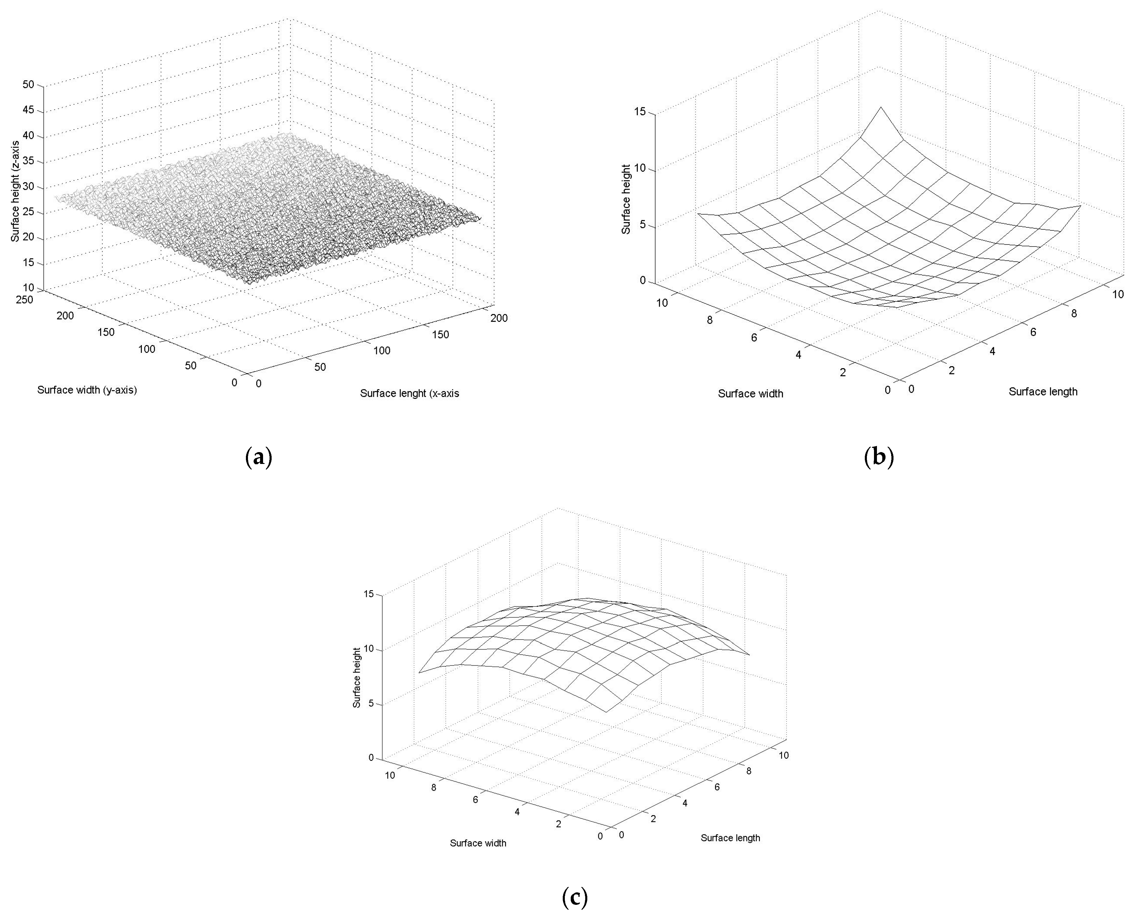
This equation system is accomplished by computing the control points P_i,j = z_i,jw_i,j which determine the convex, concave and flat Bezier surface model. From the Bezier surface model, the Hu moments are computed to determine the Hu moments pattern of the convex, concave and flat surface. For instance, the Hu moments are computed to define the Hu moments pattern of the flat surface. In this way, Equations (1)–(10) are computed from the flat surface shown in Figure 2a which includes random roughness. Thus, the results of the Hu moments for the flat surface are ϕ₁ = 0.0964, ϕ₂ = 0.0093, ϕ₃ = 1.0770 × 10⁻⁸, ϕ₄ = 1.0398 × 10⁻⁸, ϕ₅ = 1.0426 × 10⁻¹⁶, ϕ₆ = 1.8066 × 10⁻¹⁰ and ϕ₇ = −1.0508 × 10⁻¹⁶. These Hu moments represent the Hu moments pattern of a flat surface. This pattern describes a flat line from ϕ₃ to ϕ₇ and an increasing function from ϕ₂ to ϕ₁. In this case, ϕ₇ can take a negative value. Moreover, a similar Hu moment pattern is obtained in a flat surface without roughness. In the same way, the Hu moments are computed to define the Hu moments pattern of the concave topography given in Figure 2b. In this case, the Hu moments for the concave surface are ϕ₁ = 0.0087, ϕ₂ = 7.5395 × 10⁻⁵, ϕ₃ = 3.1626 × 10⁻¹², ϕ₄ = 1.5968 × 10⁻¹¹, ϕ₅ = −2.3344 × 10⁻²¹, ϕ₆ = 1.1946 × 10⁻¹⁵ and ϕ₇ = 6.9730 × 10⁻²³. These Hu moments represent the Hu moments pattern of a concave surface. In this case, the Hu pattern describes a flat line from ϕ₃ to ϕ₇ but increases from ϕ₂ to ϕ₁. In this case, ϕ₅ is a negative and ϕ₇ can be negative. Moreover, a similar Hu moment pattern is obtained for a concave surface without roughness. Additionally, the Hu moments pattern of a convex surface is defined. To do so, the Hu moments are computed for the convex surface shown in Figure 2c. The results of the Hu moments are ϕ₁ = 0.0129, ϕ₂ = 1.6526 × 10⁻⁴, ϕ₃ = 3.8968 × 10⁻¹⁰, ϕ₄ = 4.0918 × 10⁻¹⁰, ϕ₅ = −5.7007 × 10⁻²⁰, ϕ₆ = 2.7008 × 10⁻¹² and ϕ₇ = −2.0500 × 10⁻²⁰. This Hu pattern describes a flat line from ϕ₃ to ϕ₇ but increases from ϕ₂ to ϕ₁. In this case, ϕ₅ is a negative and ϕ₇ can be negative. Therefore, convex and concave surfaces provide a similar Hu moment pattern. However, the position of the line projection determines if the pattern corresponds to a concaveor convex surface. The genetic algorithm to compute the control points P_i,j is described in Section 2.2.

2.2. Bezier Surface Modeling through a Genetic Algorithm

The microscale surface recognition of a Bezier surface model is accomplished through the surface contour which is retrieved at microscale through the microscope arrangement. In this way, a Bezier surface model represents the object shape under study. Thus, mathematical model is generated from the surface contour indicated in Figure 1, where (x_i,j, y_i,j and z_i,j) represent the topography coordinates, whose sub-indexes (i,j) are established in x-direction and y-direction, respectively. The Bezier model is constructed by accomplishing Equation (11) through the control points P_i,j which move the Bezier surface toward the real surface contour. In this way, the control points P_i,j = w_i,jz_i,j are determined through the weights w_i,j. These weights are determined by substituting z_i,j and (u_i,j, v_i,j) in Equation (11) and solving the next equation system

$$\left[\begin{array}{l}{S}_{s,t}(u_{0,0},v_{0,0})\\ S_{s,t}(u_{0,0},v_{0,1})\\ S_{s,t}(u_{0,0},v_{0,2})\\ \\ S_{s,t}(u_{4,4},v_{4,4})\end{array}\right]=\left[\begin{array}{l}{B}_0(u_{0,0})B_0(v_{0,0})+B_0(u_{0,0})B_1(v_{0,0})+B_0(u_{0,0})B_2(v_{0,0})+\dots +B_4(u_{0,0})B_4(v_{0,0})\\ B_0(u_{0,0})B_0(v_{0,1})+B_0(u_{0,0})B_1(v_{0,1})+B_0(u_{0,0})B_2(v_{0,1})+\dots +B_4(u_{0,0})B_4(v_{0,1})\\ B_0(u_{0,0})B_0(v_{0,2})+B_0(u_{0,2})B_1(v_{0,0})+B_0(u_{0,2})B_2(v_{0,0})+\dots +B_4(u_{0,0})B_4(v_{0,2})\\ ⋮\begin{array}{cccc}& & & \begin{array}{ccc}\begin{array}{cccc}⋮& & & \end{array}& & ⋮\end{array}\end{array}\\ B_0(u_{4,4})B_0(v_{4,4})+B_0(u_{4,4})B_1(v_{4,4})+B_0(u_{4,4})B_2(v_{4,4})+\dots +B_4(u_{4,4})B_4(v_{4,4})\end{array}\right]\left[\begin{array}{l}{w}_{0,0},z_{0,0}\\ w_{0,0},z_{0,1}\\ w_{0,0},z_{0,2}\\ ⋮\\ w_{4,4},z_{4,4}\end{array}\right].$$

(13)

For this equation system, u_i,j and v_i,j are determined via expressions given in Equation (11) and S_s,t(u_i,j,v_i,j) = z_i,j. By employing these parameters, a genetic algorithm computes w_i,j to accomplish the Bezier surface S_s,t(u,v). To do so, Equation (13) is solved via genetic algorithm to obtain the weights w_i,j which accomplish the Bezier surface model Equation (12). In this case, the genetic procedure performs an exploration inside of the research space and exploitation outside of solution space to compute the optimized weights [15]. Based on these stages, a mathematical Bezier model is performed through a genetic algorithm and surface contour data. In this way, the weights are computed via the genetic algorithm which is explicated as follows.

In the first step, the research space is defined to compute the first weights population. To do so, the Bezier surface Equation (11) is computed via w_i,j = 1 to establish the solution space of each weight. In this case, Equation (11) is calculated via P_i,j = z_i,j. Thus, if the Bezier surface Equation (11) provides a value over the surface z_i,j, the solution space is defined in the interval [0.3, 1]. However, if the Bezier surface Equation (11) provides a minor value than z_i,j, the solution space is determined in the interval [1, 7]. In this way, the Bezier surface Equation (11) has determined the solution apace interval of each weight. Then, the first population is generated by taking randomly four values from the search interval. Thus, the four data define the first parents ($𝒲$_1,k, $𝒲$_2,k), ($𝒲$_3,k, $𝒲$_4,k) whose k-index depicts the number of each generation. In this way, the first weights population is defined via first parents ($𝒲$_1,1, $𝒲$_2,1,), ($𝒲$_3,1, $𝒲$_4,1) of each weight. From this process, the first weight population has been determined.

Then, the second step performs a crossover to generate the children of current k-generation. The crossover computes the inside parents’ children via exploration and the outside parents’ children through exploitation [16]. Thus, the current children w_1+3l+4q,k are computed via parents ($𝒲$_1,k and $𝒲$_2,k) for l = 0, l = 1, q = 0 and q = 1. However, the children w_{2+l +4q,k} are computed via ($𝒲$_3,k and $𝒲$_4,k). In this way, the current children are computed by means of the next expressions

$$w_{1+3\mathit{l}+4q,k}=\{\begin{array}{l}{\mathcal{W}}_{1+2q,k}-0.5\beta ({\mathcal{W}}_{1+2q,k}-{\mathcal{W}}_{0+5\mathit{l}}),\mathrm{if} {\mathcal{W}}_{1+\mathit{l}+2q,k}<{\mathcal{W}}_{2-\mathit{l}+2q,k}\\ {\mathcal{W}}_{2+2q,k}-0.5\beta ({\mathcal{W}}_{2+2q,k}-{\mathcal{W}}_{0+5\mathit{l}}),\mathrm{if} {\mathcal{W}}_{2-\mathit{l}+2q,k}<{\mathcal{W}}_{1+\mathit{l}+2q,k}\end{array},$$

(14)

$$w_{2+\mathit{l}+4q,k}=0.5\left[\left({\mathcal{W}}_{1+2q,k}+{\mathcal{W}}_{2+2q,k}\right)+{(-1)}^{{}^{\mathit{l}}}\beta \left|{\mathcal{W}}_{1+2q,k}-{\mathcal{W}}_{2+2q,k}\right|\right],\beta =\{\begin{array}{ll}{\sqrt{2\alpha }}^{} \mathrm{if} {}_{}^{}\alpha >0.5,& \alpha \in [0,1].\\ {\sqrt{2(\alpha -1)}}_{,}^{} otherwhise& \end{array}$$

(15)

These equations are computed for l = 0, l = 1, q = 0 and q = 1. $𝒲$₀ corresponds to the minimum and $𝒲$₅ corresponds to the maximum of each weight. Additionally, the probability distribution β is computed by means of the parameter α that is generated in the interval [0, 1]. In this way, Equation (14) computes children outside parents and Equation (15) computes children inside parents. Therefore, Equations (14) and (15) compute the children (w_1,k, w_2,k, w_3,k and w_4,k) via ($𝒲$_1,k and $𝒲$_2,k) and q = 0. In the same way, Equations (14) and (15) compute (w_5,k, w_6,k, w_7,k and w_8,k) via ($𝒲$_3,k and $𝒲$_4,k) and q = 1. From this procedure, Equations (14) and (15) compute the children in each k-generation. Additionally, the Bezier surface S_s,t(u,v) should provide continuity G¹. The P_i,j should be smooth in the border [17]. These smooth points are computed by means of P_4+4×s,j = (P_4+4s−1,j + P_4+4s+1,j)/2 and P_i,4+4t = (P_i,4+4t−1 + P_i,4+4t+1)/2.

The third step computes an objective function by employing the surface S_s,t(u_i,j, v_i,j) to determine the fitness. Thus, the fitness is computed by the expression

$$\left[\begin{array}{l}{F}_{0,0}\\ \\ \\ F_{1,0}\\ \\ \\ ⋮\\ \\ F_{n/4,m/4}\end{array}\right]=\left[\begin{array}{l}\min \left\{\frac{1}{25}\sqrt{{\displaystyle \sum _{g=0}^{g=4}{\displaystyle \sum _{r=0}^{r=4}{\left[S_{0,0}(u_{i,j},v_{i,j})-z_{i,j}\right]}^2}}}\right\}\\ \\ \min \left\{\frac{1}{25}\sqrt{{\displaystyle \sum _{g=0}^{g=4}{\displaystyle \sum _{r=0}^{r=4}{\left[S_{1,0}(u_{i,j},v_{i,j})-z_{i,j}\right]}^2}}}\right\}\\ \\ \begin{array}{cccc}& & & ⋮\end{array}\\ \min \left\{\frac{1}{25}\sqrt{{\displaystyle \sum _{g=0}^{g=4}{\displaystyle \sum _{r=0}^{r=4}{\left[S_{n/4,m/4}(u_{i,j},v_{i,j})-z_{i,j}\right]}^2}}}\right\}\end{array}\right],fitness=\frac{F_{0,0}+F_{1,0}+F_{2,0}+\dots +F_{n/4,m/4}}{(n/4)(m/4)}.$$

(16)

This fitness expression is computed trough the¹ surface data z_i,j and the Bezier surface S_s,t(u_i,j,v_i,j).

Then, the fourth step selects the (k + 1)-generation parents by means of fitness. Thus, $𝒲$_1,k+1 is taken from ($𝒲$_1,k, $𝒲$_2,k) and $𝒲$_3,k+1 is taken from ($𝒲$_3,k, $𝒲$_4,k). However, $𝒲$_2,k+1 is taken (w_1,k, w_2,k, w_3,k, w_4,k) from and $𝒲$_4,k+1 is taken from (w_5,k, w_6,k, w_7,k, w_8,k).

Then, the fifth step mutates one parent to elude trapping in a local minimum. To do so, a new parent replaces the worst parent which is determined via Equation (16). In this way, the Bezier surface Equation (13) is calculated to compute the fitness via Equation (16). If fitness is enhanced, the selected worst parent is successfully mutated. Otherwise, the mutation is not achieved. Additionally, one weight is mutated from a parent that is randomly designated. To carry it out, the selected weight is substituted with a new weight in the Bezier surface Equation (13) to compute the fitness via Equation (16). If the new weight provides better fitness, the mutation is successful. Otherwise, the mutation is achieved. From this mutation procedure, the (k + 1)-generation parents have been accomplished. Moreover, Equations (14) and (15) compute the (k + 1)-generation children. With this step, the (k + 1)-generation population is determined. The procedure to determine the (k + 1)-generation population is computed iteratively until optimizing Equation (16).

To illustrate the weights optimization, the weights of the S_0,0(u_i,j,v_i,j) are determined from the topography contour given in Figure 2b. The steps to optimize the weights are described in the flowchart of Figure 3 which describes the structure of the genetic algorithm. Thus, the first step computes the first parents of the weights. This step computes Equation (11) via w_i,j = 1 to determine the search space of each weight w_i,j. Thus, if S_0,0(u_i,j, v_i,j) is over z_i,j, the research space is defined in interval [0.3, 1]. However, if the Bezier surface is under z_i,j, the search space is defined in the interval [1, 1.7]. In this case, the weights, w_0,0 = 1 and w₄,₄ = 1, are deduced from the Bezier basis functions. However, the expressions, P_4+4s,j = (P_4+4s−1,j +P_4+4s+1,j)/2 and P_i,4+4t = (P_i,4+4t−1 + P_i,4+4t+1)/2, the weights ($𝒲$_4,0, $𝒲$_4,1, $𝒲$_4,2, $𝒲$_4,3, $𝒲$_0,4, $𝒲$_1,4, $𝒲$_2,4, $𝒲$_3,4) are determined to provide continuity G¹. Thus, four values are chosen from the solution space in random form to obtain the initial parents of each weight. The first parents are pointed out in

Table 1. First generation population generated via genetic algorithm.

Pi,j	$𝒲$1,1	$𝒲$2,1	$𝒲$3,1	$𝒲$4,1	w1.1	w2,1	w3,1	w4,1	w5,1	w6,1	w7,1	w8,1
P0,1	4.7773	4.7800	4.7583	3.9536	4.1286	4.7785	4.7789	4.8174	3.1435	4.1669	4.5235	4.7871
P0,2	3.5287	2.8255	1.9636	4.2704	2.3522	3.1669	3.2724	3.7293	1.6870	2.6238	3.3893	4.3249
P0,3	3.6140	3.7200	1.7605	3.2390	2.8483	3.6670	3.6705	3.8549	1.7513	2.4157	2.6209	3.7004
P1,0	2.2926	3.6831	3.6715	4.0298	2.1644	2.9004	3.1384	4.2026	3.4689	3.8051	3.8911	4.1741
P1,1	1.9470	2.2920	1.3373	2.4125	1.8310	2.0431	2.1852	3.2480	1.3371	1.6601	1.9109	2.4792
P1,2	2.0331	3.2020	2.2460	3.8576	1.8880	2.5084	2.7590	3.6850	2.0772	2.9500	3.2875	3.9469
P1,3	6.0711	5.0629	4.8280	5.0324	4.9800	5.4444	5.6921	6.4131	4.5137	4.8863	4.9614	5.5557
P2,0	4.4185	4.2947	1.4866	1.5336	3.3928	4.3534	4.3615	4.4331	1.4474	1.5069	1.5193	2.1067
P2,1	3.1289	2.6901	1.5340	3.3676	2.6680	2.8453	2.9708	3.2359	1.5219	2.0230	2.5697	3.4520
P2,2	5.5178	4.2465	5.1380	6.6700	4.2402	4.6895	5.0558	5.5786	4.7730	5.7343	5.9294	6.6918
P2,3	6.0749	5.6100	5.9917	4.2305	5.3861	5.7350	5.9156	6.2530	4.0962	4.7596	5.3026	6.2314
P3,0	3.7742	2.8934	3.9840	2.5912	2.8176	3.2176	3.4539	3.8605	2.3545	3.2651	3.4773	4.1501
P3,1	3.1066	1.8414	1.2777	1.4801	1.7958	2.4197	2.4955	3.4937	1.2734	1.3341	1.4050	2.7164
P3,2	2.9129	3.0561	3.0618	2.3274	2.8058	2.9828	2.9981	3.2064	2.0881	2.6173	2.7638	3.3897
P3,3	3.1086	1.2363	3.1767	3.2293	1.1794	1.7222	2.2487	3.2756	2.7820	3.1970	3.2035	3.3208
fitness	0.3224	0.6652	1.1678	1.4217	1.7809	2.3323	3.2111	4.9090	5.4896	7.1749	10.0922	16.4013

. In this table, the first column indicates the control points to be optimized and the parents ($𝒲$_1,1, $𝒲$_2,1, $𝒲$_3,1, $𝒲$_4,1) are indicated in the second to fifth column. Then, the second step computes the first children by means of Equations (14) and (15). These equations are computed via parents ($𝒲$_1,k and $𝒲$_2,k) for l = 0, l = 1 and q = 0 to obtain the children (w_1,k, w_2,k, w_3,k and w_4,k). Moreover, (w_5,k, w_6,k, w_7,k and w_8,k) are computed via Equations (14) and (15) for l = 0, l = 1 and q = 1. These children are pointed out in Table 1 in the sixth to thirteenth column. Next, the third step computes the fitness through the objective function Equation (16) by means of Bezier surface S_s,t(u_i,j,v_i,j) and z_i,j. The fitness evaluation indicates that the initial population provides a low error.

Then, the fourth step determines the (k + 1)-generation parents through the current population. To do so, $𝒲$_1,k+1 is taken from ($𝒲$_1,k and $𝒲$_2,k), and $𝒲$_3,k+1 is chosen from ($𝒲$_3,k, $𝒲$_4,k). In the same way, $𝒲$_2,k+1 is selected from (w_1,k, w_2,k, w_3,k and w_4,k) and $𝒲$_4,k+1 is selected from (w_5,k, w_6,k, w_7,k and w_8,k), respectively. In this case, $𝒲$_1,2 = $𝒲$_1,1, $𝒲$_3,2 = $𝒲$_3,1, $𝒲$_2,2 = w_1,1 and $𝒲$_4,2 = w_5,1.

In the fifth step, $𝒲$_4,2 is chosen to be mutated by a new parent obtained from the search space. Thus, Equation (16) is computed to determine fitness. As fitness was improved, $𝒲$_4,2 was changed by the new parent. Then, w_2,0 was randomly determined to mutate from $𝒲$_3,2. Next, a new weight replaces w_2,0 in $𝒲$_3,2 to compute Equation (16), and it was improved. Therefore, the weight w_2,0 is changed by the new weight. Then, algorithm computes (k + 1)-generation children by means of Equations (14) and (15). Moreover, Equation (16) is computed to determine the fitness of (k + 1)-generation children.

Table 2. Second generation population computed via genetic algorithm.

Pi,j	$𝒲$1,2	$𝒲$2,2	$𝒲$3,2	$𝒲$4,2	w1.2	w2,2	w3,2	w4,2	w5,2	w6,2	w7,2	w8,2
P0,1	4.7773	4.1286	4.7583	2.7363	3.4413	4.4383	4.5722	4.7776	2.3527	3.2636	3.9482	4.8031	4.5975
P0,2	3.5287	2.3522	1.9636	3.7694	1.9998	2.6527	3.0004	3.7899	1.6586	2.7490	3.0989	3.9729	4.1833
P0,3	3.6140	2.8483	1.7605	3.6536	2.5338	3.1380	3.3748	3.6551	1.7501	2.5315	3.0352	3.9397	4.2334
P1,0	2.2926	2.1644	3.6715	2.7929	1.9997	2.2243	2.2440	3.5333	2.5505	3.1600	3.4020	3.8566	4.6253
P1,1	1.9470	1.8310	1.3373	2.1250	1.7871	1.8690	1.8967	2.5211	1.3370	1.5576	1.8690	3.0055	4.2622
P1,2	2.0331	1.8880	2.2460	2.2674	1.5818	1.9460	1.9653	2.8178	1.8023	2.2558	2.2569	2.7300	4.1903
P1,3	6.0711	4.9800	4.8280	6.7910	4.9363	5.3483	5.7853	6.2568	4.6187	5.7769	6.0519	6.8100	4.0716
P2,0	4.4185	3.3928	4.6059	2.8543	3.0938	3.8314	4.0990	4.4219	2.7964	3.4144	4.0651	4.6444	4.2639
P2,1	3.1289	2.6680	1.5340	2.3397	2.0968	2.8553	2.9337	3.3264	1.4366	1.9030	2.1008	2.7721	4.0849
P2,2	5.5178	4.2402	5.1380	6.1288	4.1506	4.5613	4.9948	5.9815	4.7658	5.4646	5.6353	6.3440	4.0963
P2,3	6.0749	5.3861	5.9917	4.8183	4.6421	5.6249	5.8653	6.0755	4.4173	5.2168	5.4574	6.1211	3.8562
P3,0	3.7742	2.8176	3.9840	4.0754	2.6532	3.1648	3.3098	3.9525	3.4286	4.0254	4.0311	4.0868	4.3741
P3,1	3.1066	1.7958	1.2777	1.7333	1.7056	2.1418	2.7726	3.3674	1.2461	1.4267	1.5330	2.6698	3.9306
P3,2	2.9129	2.8058	3.0618	2.1111	2.0253	2.8559	2.8778	3.0425	1.7954	2.4762	2.8058	3.1492	3.7650
P3,3	3.1086	1.1794	3.1767	3.3495	1.1421	1.9837	2.3739	3.2132	2.4318	3.2527	3.2940	3.4383	3.5289
fitness	0.3224	1.7809	1.1678	5.4896	0.7635	0.9486	1.0912	1.3764	1.8031	2.2433	2.8813	4.3100	0.000342

provides the population of (k + 1)-generation. Where, the (k + 1)-generation corresponds to the second generation. In the same way, the procedure to obtain the (k + 1)-generation population is computed iteratively to minimize Equation (16). Table 2 includes the optimal control points in column fifteenth. Thus, the Bezier surface S_0,0(u,v) is defined by the optimal control points P_i,j = w_i,jz_i,j. From this procedure, the Bezier surface is generated through weight provided by the genetic algorithm. In the same procedure, the weights of the Bezier basis function S_1,0(u,v), …, S_n/4,0(u,v), …, S_n/4,m/4(u,v) are determined to construct the Bezier model Equation (12). In this way, the Bezier model has been accomplished via weights. The optical setup to retrieve three-dimensional surfaces via an optical microscope is described in Section 2.3.

2.3. Micro-Scale Surface Recovering via Micro Laser Line Projection

The optical setup to retrieve contour topography at microscale is exposed in Figure 4a. This microscopic vision system is implemented by means through an optical microscope that includes a digital camera and a laser line projector. This optical microscope is placed on a movement system which is moved through a computer to scan the surface via projector line. In this microscope setup, the topography area is established in x and y axis but the object height is indicated in z-direction. The microscope geometry in x-direction is depicted in Figure 4b. The laser diode projects a 40 μm line on the object contour which is reflected on the CCD array through the microscope. In this case, the symbol θ represents the microscope alignment angle. Moreover, the length d₀ depicts the distance between the topography point O and the objective lens. The length d₁ depicts the length from the intermediate plane to the first objective lens but F₁ indicates the objective focus position. Length L depicts the length defined from the ocular lens to the intermediate image plane. The length d₂ depicts the length defined from the CCD array to ocular lens and F₂ indicates the ocular focus position. The lateral configuration of the microscope arrangement in y-axis is shown in Figure 4c. The position of the laser line in the image plane is indicated by (x_i,j, y_i,j).

The coordinates (x_c and y_c) represent the center of the image plane, and the pixel dimension is depicted by the symbol η. The surface height z_i,j and the coordinate y_i,j are defined based on the geometry depicted in Figure 4b,c. Thus, (z_i,j and y_i,j) are computed by the equations

$$z_{i,j}=\frac{\eta (x_{i,j}-x_c)F_1{F}_2}{(F_1-d_1)(d_2-F_2)sin\theta }+O,$$

(17)

$$y_{i,j}=\frac{\eta (y_{i,j}-y_c)F_1{F}_2}{(F_1-d_1)(d_2-F_2)}+\eta y_c.$$

(18)

The surface length x_i,j is given by the slider device in the x-direction. Based on Equations (17) and (18), the surface height z_i,j and the coordinate y_i,j are computed through the vision parameters (x_c, y_c, η, θ, d₁, F₁, d₂ and F₂). These parameters are computed from Equations (17) and (18) through the genetic algorithm steps which are mentioned as follows.

The first step computes the solution space of each parameter. From the image size, the maximum and minimum are determined for the parameters (x_c, y_c, η). However, the search space of the microscope parameters (d₁, F₁, d₂ and F₂,θ) is obtained by means of the microscope geometry. In this way, the ocular lens ratio provides the minimum F₂, but two times the ocular lens ratio provides the maximum F₂. Moreover, the ocular ratio provides the minimum d₂, but four times the ocular ratio provides the maximum d₂. In the same way, the objective lens ratio provides the minimum F₁, and two times the objective ratio provides the maximum F₁. Moreover, objective ratio produces the minimum d₁, and four times the objective ratio produces the maximum d₁. Moreover, the minimum θ is established as 12°, and maximum θ is established as 50°. Thus, the research space has been obtained. From this search space, four parents ($𝒲$_1,k, $𝒲$_2,k, $𝒲$_3,k and $𝒲$_4,k) are randomly taken for each vision parameter. Thus, the four values of each parameter (x_c, y_c, η, θ, d₁, F₁, d₂ and F₂) are determined as the first parents. Then, the second step computes Equations (14) and (15) to generate the current children. To do so, ($𝒲$_1,k and $𝒲$_2,k) are replaced in Equations (14) and (15) to compute (w_1,k, w_2,k, w_3,k and w_4,k) by employing l = 0, l = 1 and q = 0. Moreover, ($𝒲$_3,k) are replaced in Equations (14) and (15) to compute (w_5,k, w_6,k, w_7,k and w_8,k) by employing l = 0, l = 1 and q = 1. Then, the third step evaluates the fitness through the microscope parameters by the next equations

$$O{b}_1=\min \left\{\frac{1}{mxn}{{\displaystyle \sum _{i=}^n{\displaystyle \sum _{j=0}^m\left[(z_{i,j}-z_{i,m})-\frac{\eta (x_{i,j}-x_c)F_1{F}_2}{(F_1-d_1)(d_2-F_2)sin\theta }+\frac{\eta (x_{i,m}-x_c)F_1{F}_2}{(F_1-d_1)(d_2-F_2)sin\theta }\right]}}}^2\right\},$$

(19)

$$O{b}_2=\min \left\{\frac{1}{mxn}{{\displaystyle \sum _{i=}^n{\displaystyle \sum _{j=0}^m\left[(y_{i,j}-y_{i,m})-\frac{\eta (y_{i,j}-y_c)F_1{F}_2}{(F_1-d_1)(d_2-F_2)}+\frac{\eta (y_{i,m}-y_c)F_1{F}_2}{(d_1-F_1)(d_2-F_2)}\right]}}}^2\right\}.$$

(20)

These equations are computed by employing the known data (z_i,j – z_i,m) and (y_i,j − y_i,1), but the fitness is calculated by the expression Obj = (Ob₁ + Ob₂)/2. Then, the fourth step generates the (k + 1)-generation population. Thus, $𝒲$_1,k+1 is chosen from ($𝒲$_1,k and $𝒲$_2,k), and $𝒲$_3,k+1 is chosen from ($𝒲$_3,k, $𝒲$_4,k). In the same way, $𝒲$_2,k+1 is chosen from (w_1,k, w_2,k, w_3,k and w_4,k) and $𝒲$_4,k+1 is chosen from (w_5,k, w_6,k, w_7,k and w_8,k). Then, the fifth step mutates the worst parent determined via Equation (16). Moreover, a new parent replaces the worst parent to compute the fitness via Equations (19) and (20). If the new parent enhances the fitness, the worst parent mutation is successfully carried out. Otherwise, the mutation is not applied. In the same way, one parameter is designated in random form to be mutated. In this procedure, a new parameter replaces the selected parameter to compute Equations (19) and (20). If the new vision parameter enhances the fitness, the selected parameter is changed, if not, the mutation is not mutated applied. With this step, the mutation is finished and the (k + 1)-generation parents have been completed. Then, Equations (14) and (15) compute performed the (k + 1)-generation children. Additionally, the fitness of these children is calculated by computing Equations (19) and (20). With this step, the (k + 1)-generation population is obtained. The step to generate the (k + 1)-generation population is computed until to minimize Equations (19) and (20). Moreover, expression z_0,j = η(x_0,j − x_c) F₁ F₂/(F₁ − d₁)(f₂ − F₂)sinθ computes the length between zero and the point O. On the other hand, the laser line position (x_i,j, y_i,j) is determined from the maximum intensity in x-direction. In this way, the coordinate x_i,j is calculated from the maximum intensity in x-direction [18]. To perform this procedure, a Bezier curve is generated in x-direction from the laser intensity through the expressions

$$x(u)={\displaystyle \sum _{i=0}^N{\mathcal{C}}_i}{(1-u)}^{N-i}{u}^i{\mathrm{x}}_{i,j},{\mathcal{C}}_i={\mathcal{C}}_{i-1}(N+1-i)/i,{\mathcal{C}}_0=1,0\le u\le 1.$$

(21)

$$I(u)={\displaystyle \sum _{i=0}^N{\mathcal{C}}_i}{(1-u)}^{N-i}{u}^i{I}_{i,j},{\mathcal{C}}_i={\mathcal{C}}_{i-1}(N+1-i)/i,{\mathcal{C}}_0=1,0\le u\le 1.$$

(22)

For these equations, x_i,j represents the line pixel position in x-axis, I_i,j represents pixel intensity and N indicates the laser line width in pixels. However, the sub-indices (i, j) depict the pixel number in x and y directions. To perform the fitting, x_i,j and I_i,j are substituted in Equations (21) and (22), respectively. In this way, a concave curve {x(u), I(u)} is generated. For this curve, I″(u) is positive in the interval 0 ≤ u ≤ 1. Therefore, the Bezier curve maximum is calculated through the derivative I′(u) = 0. For this derivative, u is computed through the Bisection algorithm. Thus, u is substituted in Equation (21) to compute x(u) which represents the line position x_i,j = x(u) in x-direction. The coordinate y_i,j is taken from the number of rows in y-direction. Moreover, the laser line edges y_i,0 and y_i,m are computed through the first derivative in y-direction. Thus, Equation (17) computes the object height z_i,j by means of x_i,j, and Equation (18) computes the surface width y_i,j by employing y_i,j. Thus, z_i,j and y_i,j have been computed through the laser line image which is provided by the camera. However, the slider device provides the surface length x_i,j. Thus, the microscale contouring has been computed.

In the microscope system, the radial distortion is deduced via line coordinate x_i,j. The coordinate x_i,j is calculated via Equations (21) and (22), and y_i,j is obtained through the row number. In this way, the distortion is calculated from the expressions x_i,j = x_i,j + δx_i and y_i,j = y_i,j + δy_j. Thus, the distortion is represented by (δx_i, δy_j), and (x_i,j, y_i,j) represent the distorted coordinates. Additionally, a line shifting is given by the expression s_i,j = (x_1,j + δx₁) − (x_i,j + δx_i), but a distorted line shifting is represented by S_i,j = x_1,j − x_i,j. From these expressions, δx_i = (x_1,j − x_i,j) − s_i,j + δx₁ = S_i,j − s_i,j + δx₁ is obtained to compute the distortion in x-direction. Furthermore, the first line shifting is obtained without distortion by projecting the line by position of the coordinate x_c where δx₁ = 0 and s_1,j = S_1,j. In this way, the line shifting s_i,j is calculated through the first shifting by the expression S_1,j by s_i,j = i × S_1,j. Thus, the distortion in x-direction is determined by the expression δx_i = (x_1,j − x_i,j) − i × S_1,j. In the same way, the distortion in direction of y-axis is deduced through the expressions (y_i,1 − y_i,j) = (y_i,1 + δy₁) − (y_i,j + δy_j) and T_i,j = (y_i,1 − y_i,j). From these expressions, δy_j = (y_i,1 − y_i,j) − j × T_i,1 is obtained to calculate the distortion in y-axis. In Section 3, the results of microscale convex, concave and flat surface recognition via Hu moments patterns are described.

3. Results

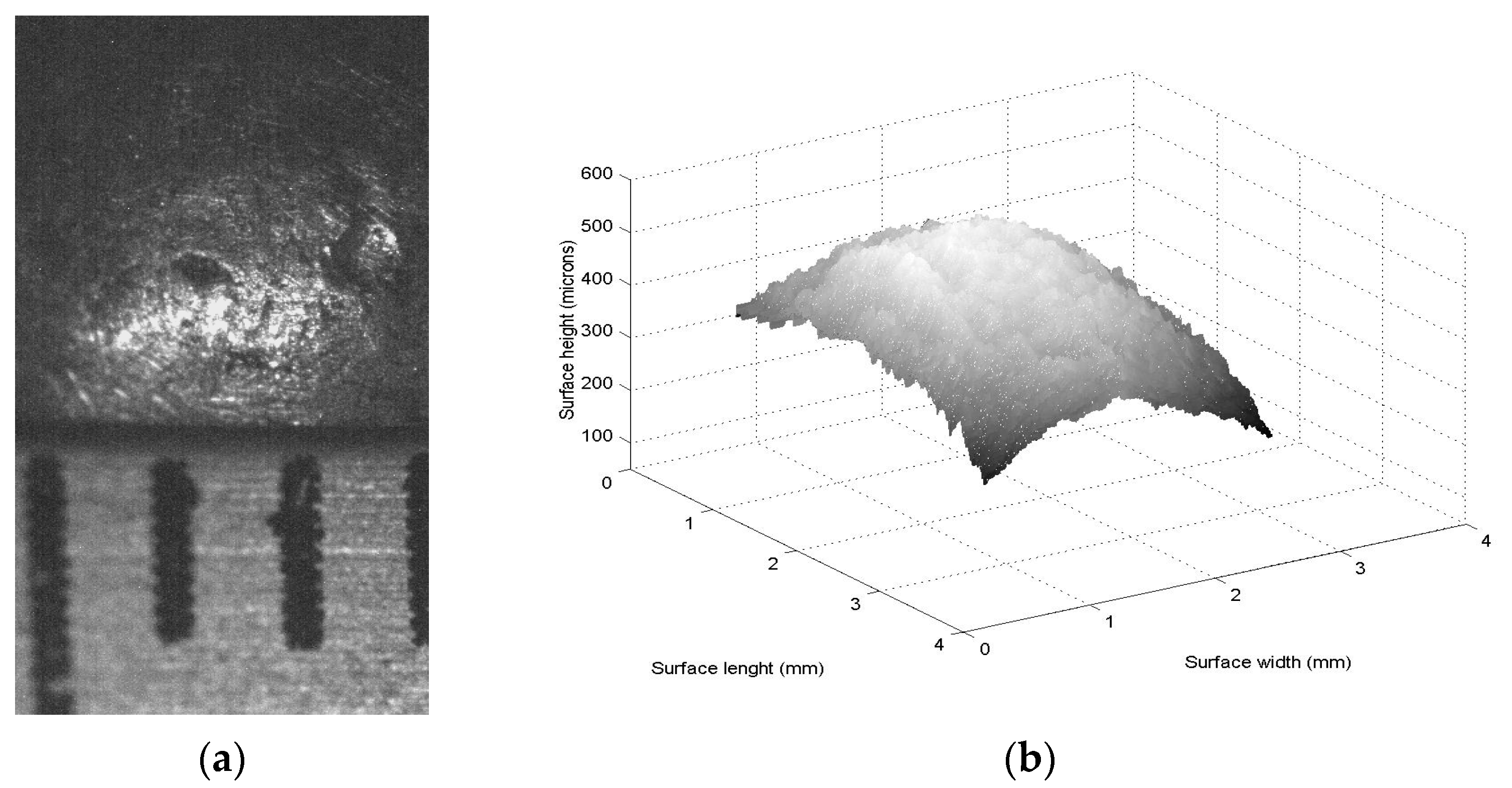
The microscale convex, concave and flat surface recognition is computed by means of the microscope setup given in Figure 4a. The surface recognition is performed on concave, convex and flat metallic iron. In this way, the first shape recognition at the microscale is carried out for the convex iron surface which is illustrated in Figure 5a, where the scale in the x-axis is indicated in mm. Figure 5b shows a laser line projected on the iron surface. In this way, surface recognition is performed through the surface contour which is recovered via the microbe vision system. To retrieve the surface contour, the iron topography is scanned by the laser line in the x-direction. In this procedure, the camera aquires the line reflection to calculate the coordinates (x_i,j and y_i,j) by the means of Equations (21) and (22). Then, Equation (17) computes the surface high z_i,j through the x_i,j, and Equation (18) computes the surface width y_i,j through the y_i,j. Additionally, the slider device provides the coordinate x_i,j. In this way, two hundred and sixteen laser lines were employed to compute the contour topography shown in Figure 5c. The scale of x and y axis are indicated in mm, but the scale of the z-axis is given in microns. The contouring accuracy is defined via relative error [19] which is determined based on measurements given by a physical contact process. Thus, the error of the contour measurement is computed through the next equation

$$Error\%=\frac{100}{n\cdot m}{\displaystyle \sum _{i=0}^n{\displaystyle \sum _{j=0}^m\frac{\left|z_{i,j}-h_{i,j}\right|}{h_{i,j}}}},$$

(23)

where h_i,j is given by the contact procedure, z_i,j is determined through Equation (17) and n·m depicts the number of computed data. Then, the relative error is computed via Equation (23) for the surface given in Figure 5c, and the result is a relative error of 0.883%.

Then, a Bezier model is built via a genetic algorithm by employing the topography data shown in Figure 5c as described in Section 2.3. To do so, the first step determines the search space and the first parents of each weight. Thus, the search space is established in the interval [0.3, 1.7] for each weight. From the search space, four parents are randomly chosen for the weights of the functions S_s,t(u,v). However, the second step computes Equations (14) and (15) for l = 0, l = 1, q = 0 and q = 1 to create the first children. Then, the third step replaces the control points P_i,j = z_i,jw_i,j in Equation (11) to compute the fitness via Equation (16). Then, the fourth selects the (k + 1)-parents, where $𝒲$_1,k+1 and $𝒲$_3,k+1 are selected from ($𝒲$_1,k, $𝒲$_2,k) and ($𝒲$_3,k, $𝒲$_4,k), respectively. Moreover, $𝒲$_2,k+1 and $𝒲$_4,k+1 are collected from (w_1,k, w_2,k, w_3,k and w_4,k) and (w_5,k, w_6,k, w_7,k and w_8,k), respectively. Then, the fifth step mutates the lowest fitness parent which is chosen through Equation (16). Thus, a new parent replaces the worst parent to compute Equation (16). If the new parent improves the fitness, the worst parent is mutated, if not, the mutation is not applied. In the same way, one weight is selected to be mutated from a parent that is randomly selected. To carry it out, a new weight replaces the selected weight to compute Equation (16) which determines the fitness. Thus, if the new weight enhances fitness, the selected weight is changed, if not, the mutation is not applied. Then, the second step computes Equations (14) and (15) to generate the (k + 1)-generation children. The fitness of these children is computed via Equation (16). The procedure to compute the (k + 1)-generation population is computed iteratively to find the weights which minimizes Equation (16). In this way, 247 generations were calculated to accomplish the Bezier model. Then, the optimal P_i,j = z_i,jw_i,j is replaced in Equation (11) to determine the Bezier model that computes the topography contour shown in Figure 5d. The Bezier model accuracy is determined by computing Equation (23), where z_i,j is determined via Equation (17), h_i,j is computed via S_s,t(u, v) and the number of data is represented by n·m. In this case, the Bezier model provides a relative error of 0.9012% with respect to the iron topography given in Figure 5c. Then, the Hu moments are computed from the Bezier surface to determine the Hu moments pattern. In this way, Equations (1)–(10) are computed from the Bezier surface shown in Figure 5d. Thus, the Hu moments are computed, and the results are ϕ₁ = 0.0098, ϕ₂ = 9.5861 × 10⁻⁵, ϕ₃ = 8.8027 × 10⁻¹¹, ϕ₄ = 5.7037 × 10⁻¹⁴, ϕ₅ = 5.3374 × 10⁻²⁵, ϕ₆ = −5.4946 × 10⁻¹⁷, ϕ₇ = −1.4123 × 10⁻²⁵. This Hu pattern describes a flat pattern from ϕ₃ to ϕ₇, but, and increases from ϕ₂ to ϕ₁. In this case, ϕ₅ is negative, and ϕ₇ is negative. Therefore, the Hu moments pattern can be a convex or a concave surface as pointed out in Section 2.1. However, laser line position x_i,0 and x_i,m corresponds to a maximum position in the x-axis; therefore, the Hu pattern corresponds to a convex surface. Thus, the surface shown in Figure 5d has been recognized as a convex surface through the Hu moments pattern.

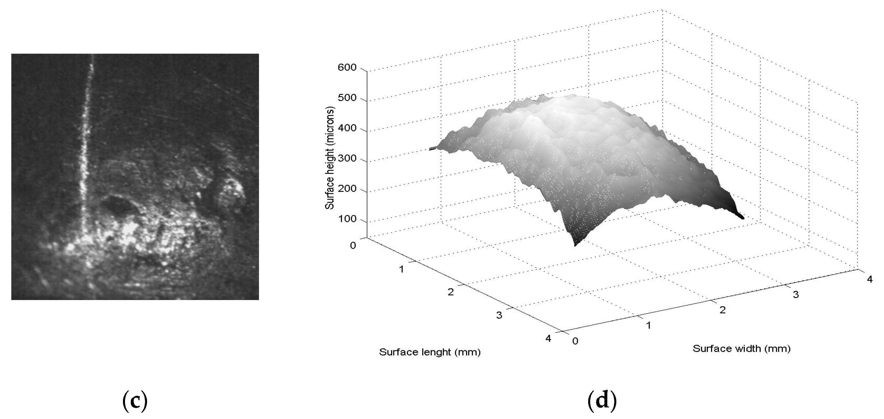
The second surface recognition is carried out for the metallic iron topography shown in Figure 6a. However, Figure 6b illustrates the laser line projected on the iron topography. In this way, the iron topography is scanned in the x-direction. During the scanning, the coordinates (x_i,j and y_i,j) are computed via Equations (21) and (22). Then, Equation (17) computes z_i,j by employing x_i,j, and Equation (18) computes y_i,j by the means of y_i,j. However, the slider device provides x_i,j. Thus, two hundred and twenty images were employed to compute the topography contour shown in Figure 6c. The scale of the x and y axis are given in mm, but the scale of the z-axis is indicated in microns. The relative error of the surface contouring is determined by computing Equation (23),where z_i,j is the topography contour computed by Equation (17) and h_i,j indicates the reference surface. Thus, the relative is calculated via Equation (23), and the accuracy is a relative error of 0.7362%. Then, the Bezier model is generated by employing the contour data given in Figure 6c where the control points P_i,j = z_i,jw_i,j are computed via genetic algorithm. In this way, the first step defines the search space in the interval [0.3, 1.7] for each weight. From this search space, four parents are randomly taken for each weight of the Bezier surface Equation (11). Then, the second step computes the crossover via Equations (14) and (15) to create the first children. Then, the third step computes Equation (16) via points P_i,j = z_i,jw_i,j to determine the fitness. Then, the fourth step selects the (k + 1)-generation parents via fitness., $𝒲$_1,k+1, $𝒲$_3,k+1, $𝒲$_2,k+1, and $𝒲$_4,k+1 are collected from ($𝒲$_1,k, $𝒲$_2,k), ($𝒲$_3,k, $𝒲$_4,k), (w_1,k, w_2,k, w_3,k, w_4,k) and (w_5,k, w_6,k, w_7,k, w_8,k), respectively. Then, the fifth step mutates the lowest fitness parent that is chosen by computing Equation (16). Thus, if the fitness is improved through the mutation, the worst parent is changed by the new parent, if not, the mutation is not applied. Moreover, one weight is selected to be mutated from a parent that is determined random form. Thus, a new weight replaces the selected weight to compute Equation (16). Thus, if the fitness is improved by the new weight, the selected weight is changed by the new weight.

Then, the second step computes the children of the (k + 1)-generation via Equations (14) and (15). The procedure to compute the (k + 1)-generation population is repeated to minimize the objective function Equation (16) where 203 iterations were performed to obtain the optimal weights. Thus, the optimal control points P_i,j = z_i,jw_i,j are replaced in Equation (11) to compute the topography contour shown in Figure 6d. The Bezier model accuracy is computed via Equation (23), where z_i,j is the computed by Equation (17), and h_i,j is the Bezier surface S_s,t(u, v). In this case, the Bezier model provides a relative error of 0.8651%. Then, the Hu moments pattern is computed from the Bezier surface data given in Figure 6d. Thus, Equations (1)–(10) are computed from the contour data shown in Figure 6d. The result of these Hu moments are ϕ₁ = 0.0061, ϕ₂ = 3.7308 × 10⁻⁵, ϕ₃ = 1.6666 × 10⁻¹², ϕ₄ = 1.6949 × 10⁻¹², ϕ₅ = 2.9203 × 10⁻²⁴, ϕ₆ = 1.8667 × 10⁻¹⁵ and ϕ₇ = −2.8675 × 10⁻²⁴. This pattern describes a flat line from ϕ₃ to ϕ₇, but an increasing function from ϕ₂ to ϕ₁. In this case, ϕ₇ is a negative value. Therefore, the Hu moment pattern is established as a flat surface as pointed out in Section 2.1. Thus, the surface shown in Figure 6d has been recognized as a flat surface through the Hu moments pattern.

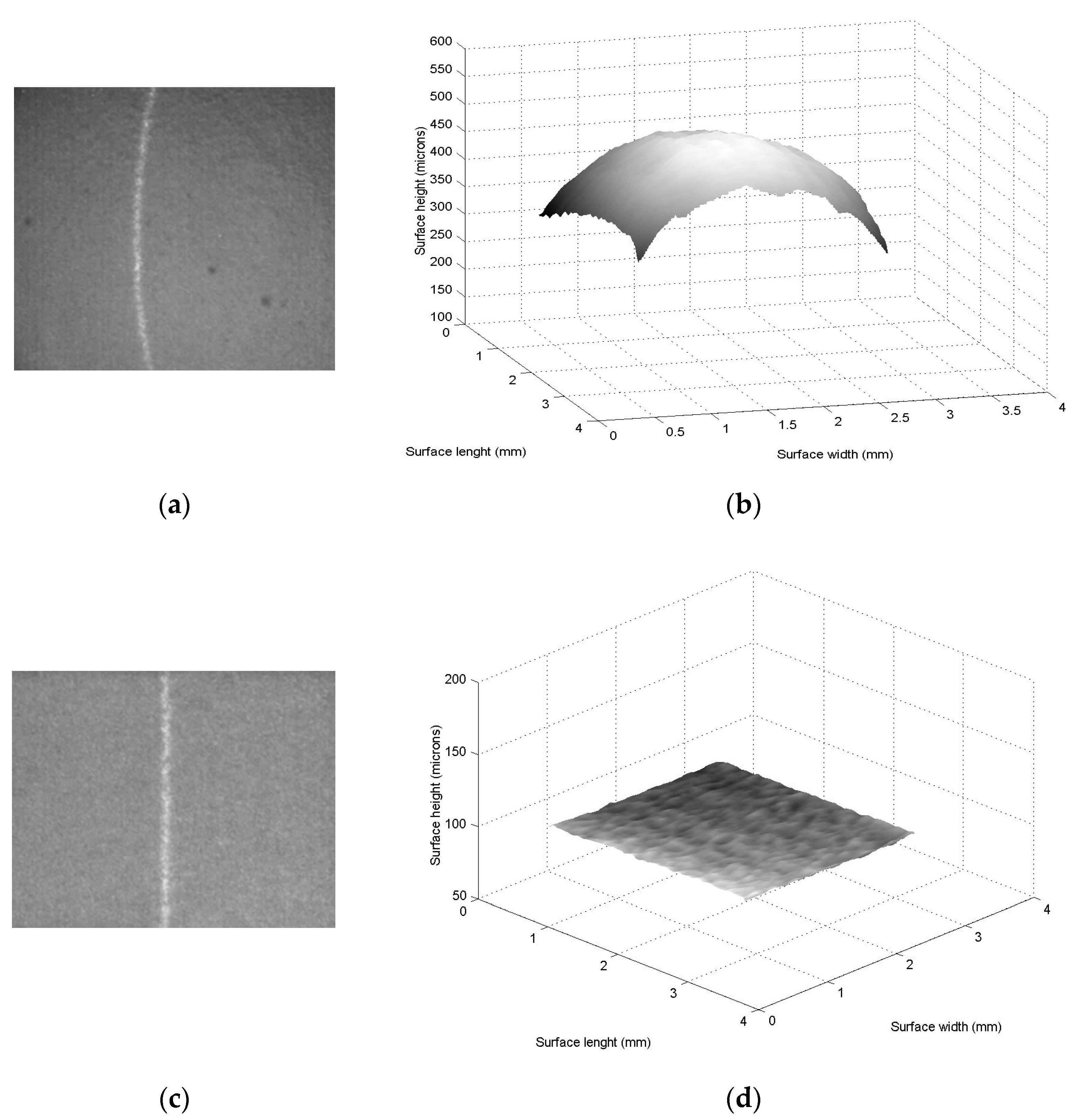
The third iron surface recognition at microscale is computed for the concave topography shown in Figure 7a. However, Figure 7b shows the microlaser line projected on the iron object. To perform the recognition, the object topography is retrieved via laser line scanning in the x-direction. From the scanning, the coordinates (x_i,j and y_i,j) are computed by Equations (21) and (22). Then, Equation (17) computes z_i,j through the position x_i,j, and Equation (18) computes y_i,j through the position y_i,j. However, the slider device provides the coordinate x_i,j. In this case, two hundred and fourteen images were employed to retrieve the topography shown in Figure 7c, where the scale of the x and y axis are given in mm, but the scale of the z-axis is given in microns. The relative error of the contoured surface is calculated via Equation (23) by employing the reference surface h_i,j. Thus, Equation (23) is computed, and the result is a relative error of 0.902%. Then, the Bezier model is computed from the contour data given in Figure 7c. Thus, the control points P_i,j = z_i,jw_i,j are computed via genetic algorithm, where the first step determines the search space in the interval [0.3, 1.7], and four parents are randomly taken for each weight w_i,j. Then, the second step computes the first children via crossover Equations (14) and (15). Then, the third step computes the fitness Equation (16) via control points P_i,j = z_i,jw_i,j. Then, the fourth step selects ($𝒲$_1,k+1, $𝒲$_3,k+1, $𝒲$ _2,k+1 and $𝒲$_4,k+1) from ($𝒲$_1,k and $𝒲$_2,k), ($𝒲$_3,k and $𝒲$_4,k), (w_1,k, w_2,k, w_3,k and w_4,k) and (w_5,k, w_6,k, w_7,k and w_8,k). Then, the lowest fitness parent is mutated in the fifth step. Moreover, one weight designated in random form is mutated. Then, the second step computes the (k + 1)-generation children via Equations (14) and (15). The procedure to compute the (k + 1)-generation population is computed iteratively to minimize Equation (16). In this procedure, 228 generations were employed to compute the optimal weights. Then, the Bezier model Equation (11) is computed by employing P_i,j = z_i,jw_i,j to obtain the surface shown in Figure 7d. The relative error of this Bezier surface is computed via Equation (23), where z_i,j is determined by Equation (17) and h_i,j is the Bezier surface S_s,t(u,v) computed via Equation (11). Thus, the Bezier surface model provides a relative error of 0.981%. Then, the Hu moments pattern is determined from the Bezier surface. In this way, Equations (1)–(10) are computed from the contour topography data given in Figure 6d to establish the Hu moments pattern. The results are ϕ₁ = 0.0128, ϕ₂ = 1.6507 × 10⁻⁴, ϕ₃ = 4.1305 × 10⁻¹⁰, ϕ₄ = 4.3164 × 10⁻¹⁰, ϕ₅ = −4.4624 × 10⁻²⁰, ϕ₆ = 2.9023 × 10⁻¹² and ϕ₇ = −3.4863 × 10⁻²⁰. This Hu pattern describes a flat pattern from ϕ₃ to ϕ₇, but increases from ϕ₂ to ϕ₁. In this case, ϕ₅ is negative and ϕ₇ is negative. Therefore, the Hu moments pattern can be a convex or a concave surface as pointed out in Section 2.1. However, the laser line position x_i,0 and x_i,m correspond to a minimum position in the x-axis; therefore, the Hu pattern corresponds to a concave surface. Thus, the surface shown in Figure 7d has been recognized as a concave surface through the Hu moments pattern.

Additionally, the surface recognition at microscale is computed on materials, such as plastic and paper. Thus, surface recognition is computed for the plastic topography shown in Figure 8a. To do so, the plastic surface is retrieved is scaned in x-axis, where the coordinates (x_i,j, y_i,j) are computed by Equations (21) and (22). Then, Equation (17) computes surface height z_i,j, Equation (18) computes the coordinate y_i,j, but the slider device provides surface width x_i,j. In this case, two hundred and twenty two images were employed to retrieve the surface. The surface accuracy is computed via Equation (23), and the result is a relative error of 0.896%. Next, the Bezier model is computed from the surface height z_i,j by computing the control points P_i,j = z_i,jw_i,j through the genetic algorithm. To do so, the search space is determined in the first step in the interval [0.3, 1.7] and four parents are randomly taken for each weight w_i,j.

The second step computes Equations (14) and (15) to determine the first children. The third step computes the fitness Equation (16) via control points P_i,j = z_i,jw_i,j. Then, the fourth step selects ($𝒲$_1,k+1, $𝒲$_3,k+1, $𝒲$ _2,k+1 and $𝒲$_4,k+1) from ($𝒲$_1,k and $𝒲$_2,k), ($𝒲$_3,k and $𝒲$_4,k), (w_1,k, w_2,k, w_3,k and w_4,k) and (w_5,k, w_6,k, w_7,k and w_8,k). Then, the fifth step mutates the lowest fitness parent, and one weight from a parent which is randomly selected. Then, the second step computes the (k + 1)-generation children through Equations (14) and (15). Thus, the procedure to generate the (k + 1)-generation population is computed iteratively to minimize Equation (16). In this procedure, 238 iterations were computed to find the optimal weights. Then, the Bezier model Equation (11) is computed by means of P_i,j = z_i,jw_i,j to obtain the surface shown in Figure 8b. The relative error of this Bezier surface is computed through Equation (23), where z_i,j is computed via Equation (17) and h_i,j is the Bezier surface S_s,t(u,v) computed via Equation (11). Thus, the Bezier surface model provides a relative error of 0.932%. Then, the Hu moments pattern is determined from the Bezier surface shown in Figure 8b. In this way, Equations (1)–(10) are computed from the Bezier surface to establish the Hu moments pattern. The results are ϕ₁ = 0.0096, ϕ₂ = 9.2463 × 10⁻⁵, ϕ₃ = 1.8333 × 10⁻¹¹, ϕ₄ = 4.1469 × 10⁻¹², ϕ₅ = −5.0870 × 10⁻²², ϕ₆ = 5.4574 × 10⁻¹⁶ and ϕ₇ = 2.3880 × 10⁻²³. This Hu pattern describes a flat pattern from ϕ₃ to ϕ₇, but increases from ϕ₂ to ϕ₁. In this case, ϕ₅ is negative. Therefore, the Hu moments pattern can be a convex or a concave surface as pointed out in Section 2.1. However, the line position x_i,0 and x_i,m correspond to a maximum position in the x-axis; therefore, the Hu pattern corresponds to a convex surface. Thus, the topography contour shown in Figure 8b has been recognized as a convex surface through the Hu moments pattern.

In the same way, the microscale surface recognition is computed for the paper surface given in Figure 8c. This procedure is carried out by scanning the paper topography in the x-direction to compute the coordinates (x_i,j, y_i,j) through Equations (21) and (22). Then, (z_i,j, y_i,j) are computed via Equations (17) and (18), but x_i,j is collected from the slider device. In this case, two hundred and eighteen images were employed to compute the surface topography. The surface accuracy is determined by computing Equation (23) which provides a relative error of 0.921%. Then, the Bezier surface is computed from the surface z_i,j by computing the control points P_i,j = z_i,jw_i,j. Thus, the first step determines the search space in the interval [0.3, 1.7] and four parents are randomly taken for each weight w_i,j. The second step computes the first children via Equations (14) and (15). The third step computes the fitness Equation (16). Then, the fourth step selects ($𝒲$_1,k+1, $𝒲$_3,k+1, $𝒲$ _2,k+1 and $𝒲$_4,k+1) from ($𝒲$_1,k and $𝒲$_2,k), ($𝒲$_3,k and $𝒲$_4,k), (w_1,k, w_2,k, w_3,k and w_4,k) and (w_5,k, w_6,k, w_7,k and w_8,k), respectively. Then, the fifth step mutates the lowest fitness parent and one weight from a parent which is randomly selected. Then, the second step computes the (k + 1)-generation children via Equations (14) and (15). Thus, the procedure to generate the (k + 1)-generation population is computed iteratively to minimize Equation (16). Thus, 208 generations were computed to determine the optimal weights. Then, the Bezier model Equation (11) is computed via the means of P_i,j = z_i,jw_i,j to obtain the surface topography shown in Figure 8d. The relative error of this topography is computed via Equation (23), where z_i,j is computed via Equation (17) and h_i,j is the Bezier surface S_s,t(u, v) computed via Equation (11). Thus, the Bezier surface model provides a relative error of 0.952%. Then, the Hu moments pattern is determined from the Bezier surface shown in Figure 8d. Thus, Equations (1)–(10) are computed from the Bezier surface to establish the Hu moments pattern. The result of these Hu moments are ϕ₁ = 0.0059, ϕ₂ = 3.4819 × 10⁻⁵, ϕ₃ = 3.5756 × 10⁻¹¹, ϕ₄ = 3.5594 × 10⁻¹¹, ϕ₅ = 1.2611 × 10⁻²¹, ϕ₆ = 3.7812 × 10⁻¹⁴ and ϕ₇ = −1.2610 × 10⁻²¹. This Hu pattern describes a flat line from ϕ₃ to ϕ₇, but an increasing function from ϕ₂ to ϕ₁. In this case, ϕ₇ is a negative value. Therefore, the Hu moment pattern is established as a flat surface as pointed out in Section 2.1. Thus, the paper surface shown in Figure 8d has been recognized as a flat surface through the Hu moments pattern.

To elucidate the validity of the proposed microscale surface recognition, the advantages over the optical microscope imaging systems are described as follows. Firstly, the Hu moments pattern and microlaser provide a recognition accuracy of a relative error of 0.674% for microscale concave, convex and flat surface recognition, where the recognition accuracy is computed via a relative error in Equation (23). In this case, Equation (23) is computed by employing the Hu moments provided on the surface contoured via microlaser line projection and Hu moments provided by the surface contoured through a contact method. This recognition accuracy represents an advantage over the optical microscope imaging systems which provide a relative error of over 2%. Secondly, the Hu moments pattern and microlaser line provide good robustness for characterizing microscale concave, convex and flat surface patterns. In this matter, a flat surface contoured via microlaser line produces always the same Hu moments pattern. Therefore, the microscale flat surface is always recognized with a small relative error of 0.527%. In the same way, the Hu moments pattern always provides the same pattern for a concave and convex surface. However, the laser line position in the x-direction determines if the topography is concave or convex. In this way, the microscopic convex and concave surface are always recognized with a small relative error of 0.674%. This robustness is not provided by optical microscope systems based on image processing. It is because the Hu moments pattern varies with the image intensity variation. In this way, the robustness characterizing represents an advantage over the optical microscope imaging systems. Thirdly, the contouring based on a microscopic laser line provides the real surface shape at microscale. This contouring accuracy is achieved because the microlaser line reflects the real object contour on the camera image plane. Instead, the optical microscope imaging systems do not depict the topography contour accurately and the surface recognition is not so accurate. Therefore, surface contouring represents an advantage over the optical microscope systems which determine topographic data by means of gray-level image processing. Fourthly, the simple method for surface recognition provides a very easy form to perform the surface recognition, where the recognition procedure is performed by computing Hu moments for Equations (4)–(10) from a Bezier surface which is computed from surface data contoured via laser line scanning. Instead, the image processing of an optical microscope requires complicated procedures and great quantity of sampled images to perform the training procedures. Therefore, the recognition structure based on the Hu moments pattern and the microlaser line provides a suitable structure algorithm for surface recognition at the microscale. Based on these criteria, the concave, convex and flat surface recognition at the microscale has been achieved in a good manner. A discussion of the viability of the proposed surface recognition is explained in Section 4.

4. Discussion

The viability of the surface recognition at the microscale is determined through the recognition accuracy [20,21]. Moreover, the capability of the microscale concave, convex and flat surface recognition is deduced by means of the recognition accuracy [22,23]. Therefore, the contribution of the proposed microscale surface recognition is established through recognition accuracy, where recognition accuracy is determined through surface recognition via a method based on contact [24]. Moreover, the efficiency of the recognition system structure is involved in the viability. In the proposed microscale surface recognition, the recognition accuracy and the microscope system efficiency provide good results. For instance, surface recognition via Hu moments pattern and micro laser line projection always recognizes flat metallic surfaces. It is because a flat metallic surface always produces the same Hu moments pattern which describes a flat line from ϕ₃ to ϕ₇ but an increasing value from ϕ₂ to ϕ₁. The small variations of the Hu moments pattern are produced due to the surface roughness. In this way, the variation of the Hu moments pattern for the flat surface is 0.527% which is computed through the relative error. Moreover, the recognition via Hu moments pattern and microlaser line projection always recognize concave and convex metallic surfaces. It is because concave and convex metallic surfaces always produce the same Hu moments pattern which describes a flat line from ϕ₃ to ϕ₇, where ϕ₅ is a negative value. However, the Hu moments pattern provides an increasing value from ϕ₂ to ϕ₁. Additionally, the laser line position x_i,0 and x_i,m determine if the surface is concave based on the maximum and minimum position in the x-axis. The small variation of the Hu moments pattern due to the surface roughness for the concave and convex surface is a relative error of 0.674%. To elucidate the viability of the proposed surface recognition, the accuracy of the concave, convex and flat surface recognition reported in recent years is commented on as follows. The surface recognition accuracy of the optical microscope vision system is related to surface contouring which is not included in surface recognition via microscope image processing. Typically, microscopic concave, convex and flat surface recognition is performed with a relative error of over 2.5% [25,26,27], where the surface shape is determined through microscope images based on gray level. Therefore, surface recognition is not carried out through the surface topography contour. The missing of this process reduces the surface recognition accuracy. Moreover, the traditional optical microscope techniques compute the contour data via image intensity to characterize the surface pattern [28,29]. However, the image intensity does not depict the topography contour with great accuracy. Thus, the surface pattern characterizing is not so accurate. Instead, the microlaser line reproduces the topography contour on the image plane with great accuracy. It is because the laser line reflects the real surface contour in the image plane through the microscope. This procedure leads to obtaining the same Hu moments pattern for each surface shape which includes roughness. This criterion has been corroborated through the results of the concave, convex and flat surface recognition pointed out in Section 3. On the other hand, the efficiency of the proposed surface recognition is established through the system structure to perform the surface recognition. For instance, the microlaser line contouring performs topography measurement at microscale in the accurate form. It is because the laser line reflects the topography contour in the CCD camera. Also, the Bezier surface model Equation (11) provides all necessary surface points to compute the Hu moments pattern. In this way, the Hu moments provide the same characteristic pattern for a flat surface. Moreover, the Hu moments provide the same characteristic pattern for a concave and a convex surface, where the microlaser line position establishes if the pattern corresponds to a concave or a convex surface. Thus, pattern characterization is carried out through efficient stages which produce an efficient and accurate surface recognition. It is because pattern characterization always produces the same pattern for the same surface topography. These statements have been corroborated by several microscale concave, convex and flat surface recognition trials. Instead, deep learning methods have emerged for surface recognition. The deep learning methods lie in a well-designed convolutional neural network and a huge data set of images related to the target. Thus, the recent methods based on deep learning perform pattern training through several hundred images [30] which do not produce the same pattern. It is because pattern characterization is carried out via image intensity which does not depict the surface topography in its accurate form. In this way, the pattern characterization depends on the surface reflectance, light pattern intensity and reflection angle. Thus, the training via image gray level requires several hundred samples of the same surface topography to perform pattern characterization. Thus, the suitable structure of the surface recognition via Hu moments pattern and micro laser line contouring gives a better efficiency than the surface recognition performed via pattern characterization based on gray-level images. This criterion has been corroborated through the steps of the surface recognition via Hu moments pattern and micro laser line contouring. Moreover, the capability of microscale surface recognition via Hu moments pattern has been corroborated by performing surface recognition on other materials, such as plastic and paper. In the case of the plastic surface, the laser line image depicts the real topography contour. This statement is corroborated by the microlaser line displayed in Figure 8a. Therefore, the Bezier surface model Equation (11) computes the surface topography with great accuracy and a relative error of 0.932%. Moreover, the Bezier surface produces a Hu moments pattern which is very similar to the Hu moments pattern of the metalic surface. The variation of the Hu moments pattern for the convex surface is a relative error of 0.624%. Additionally, the laser line position x_i,0 and x_i,m determine that the Hu pattern corresponds to a convex surface. Thus, it is elucidated that the microscale laser line contouring provides good surface recognition at the microscale of metals and other materials. This criterion is also elucidated by performing surface recognition on the paper surface. In the case of the paper surface, the laser line image depicts the real topography contour. This statement is demonstrated by the micro laser line illustrated in Figure 8a. Therefore, the Bezier surface model Equation (11) computes the surface topography with great accuracy and a relative error of 0.952%. Moreover, the Bezier surface produces a Hu moment pattern which is very similar to the Hu moments pattern of the flat metallic surface, where the variation of the Hu moments pattern for the flat surface is 0.502%. From these criteria, it is corroborated that the microscale surface recognition via micro laser line provides good surface recognition for different surface materials. It is the difference in recognition techniques based on microscope gray-level images, where the surface material modifies the image intensity which determines the topographic data. This limitation decreases surface recognition accuracy. Thus, the viability of the microscale concave, convex and flat surface recognition via the Hu moments pattern and microlaser line projection has been corroborated. In addition, the basic optical setup provides an inexpensive system that increases the viability of the proposed microscale concave, convex and flat surface recognition. Thus, the proposed surface recognition makes an enhancement in the field of the microscale concave, convex and flat surface recognition of the microscope imaging systems.

The concave, convex and flat surface recognition at microscale has been implemented in a computer at 2.2 GHz of velocity. This computer performs the program to capture 64 images per second via a digital camera. Moreover, the slider device is moved through a computer program. Thus, the topography transverse section is recovered in 0.0052 s by processing one laser line image. The time consumed to perform the surface recognition includes the topography contouring via laser line scanning, surface modeling and pattern characterization. Thus, the convex surface recognition of the iron topography given in Figure 5b is performed in 96.38 s, the flat surface recognition of the iron surface shown in Figure 6b is performed in 84.37 s and the concave surface recognition of the iron topography illustrated in Figure 7b is carried in 92.49 s. Additionally, the convex surface recognition of the plastic topography given in Figure 8b is performed in 98.12 s, and the recognition of the flat paper surface shown in Figure 8d is performed in 83.598 s.

5. Conclusions

A technique to make concave, convex and flat surface recognition via Hu moments pattern and microlaser line contouring has been elucidated. The surface recognition performed via microlaser line contouring enhances the surface recognition accuracy of the concave, convex and flat surface recognition which is performed via optical microscope imaging systems. This viability of microscale surface recognition has been elucidated through the surface recognition accuracy, and the efficient structure to characterize concave, convex and flat surface patterns. In this way, Hu moments pattern and the microlaser line contouring have improved the accuracy of the microscopic surface recognition of optical microscope imaging systems by reducing the relative error from 2.0% to 0.67%. It is because the microscale concave, convex and flat surface recognition is performed by means of the real topography contour. Furthermore, the algorithm structure based on the Hu moments pattern and microlaser line contouring provides a pattern characterization efficient and more robust than the pattern characterization computed by the traditional microscope imaging systems. Thus, the surface recognition via Hu moments pattern and microlaser line contouring provides a valuable tool to perform surface recognition via systems based on optical microscope. Moreover, the basic microscope arrangement makes a suitable optical setup to make microscale surface recognition which corroborates the capability of the proposed system. Thus, the concave, convex and flat surface recognition via Hu moments pattern and microlaser line projection has been performed at the microscale with good results.