Article

Evolution of Poisson’s Ratio in the Tension Process of Low-Carbon Hot-Rolled Steel with Discontinuous Yielding

Research Center for Structural Materials, National Institute for Materials Science, 1-2-1 Sengen, Tsukuba, Ibaraki 305-0047, Japan
*
Author to whom correspondence should be addressed.
Metals 2023, 13(3), 562; https://doi.org/10.3390/met13030562
Submission received: 26 January 2023 / Revised: 8 March 2023 / Accepted: 8 March 2023 / Published: 10 March 2023
(This article belongs to the Special Issue Deformation, Fracture and Microstructure of Metallic Materials)

Abstract

:
Low-carbon hot-rolled steel generally undergoes a deformation process composed of four phases, i.e., elastic deformation, discontinuous yielding, work hardening, and macroscopic plastic-strain localization in a tension test. The evolution of the Poisson’s ratio in terms of the average Poisson’s ratio and the local Poisson’s ratio in the deformation process from the non-load state to the onset point of specimen necking was investigated. The main results are as follows: (1) the average Poisson’s ratio cannot accurately represent the local Poisson’s ratio in the discontinuous-yielding phase; (2) the Poisson’s ratio varied significantly within a plastic band in the discontinuous-yielding phase, and the maximum Poisson’s ratio was reached within the plastic band; and (3) the strain rate greatly increased the Poisson’s ratio.

1. Introduction

Materials respond to stress by straining. Under an applied stress, a material deforms (expansion or contraction) in directions parallel and perpendicular to the direction of the applied stress, i.e., resulting in strains along the two directions. The negative of the ratio of the later strain to the former strain is defined as the Poisson’s ratio ( ν = s t r a i n   p e r p e n d i c u l a r   t o   t h e   a p p l i e d   s t r e s s s t r a i n   p a r a l l e l   t o   t h e   a p l l i e d   s t r e s s ) [1]. Material characteristic (anisotropy of microstructure, strain state of material) and loading conditions (strain rate, temperature) influence the ν. For instance, when the strain state of a structural steel changes from the elastic state to the plastic state in a tension process, its Poisson’s ratio greatly increases [2,3]. If the microstructure of the steel is isotropic, in this change process of strain sate, the transition of the ν is from a low value (0.27 to 0.3) [2,4] to an upper limit value (0.5) [2]. When the microstructure of an elastic media is anisotropic and the rotation of microscopic clusters in it occurs, the upper limit of the ν could exceed 0.5 [5]. The ν in the elastic state is usually a material constant [2,3,4], but it is a function of the applied strain in the large plastic strain regime [3,6]. The influence of the strain rate on the ν depends on the material types: an enhanced strain rate decreases the ν of porous titanium [7] and polymeric foams [8] but increases that of polyoxymethylene [9]. The strain rate hardly affects the ν of shale [10]. Test temperature is another factor influencing the ν. Raising the test temperature increases the ν of 8–18 stainless steel [11].
Structural steels are widely used in engineering structures, such as bridges, ships, oil tanks, and so on. To ensure the integrity of structures, steels are commonly designed to be in service in the elastic strain regime [12]. Therefore, as an elastic constant, the ν is mainly concerned with the elastic deformation region, and only the ν in the elastic regime is given in data handbooks [4,11]. However, a database on the evolution of the ν in a whole deformation process is important in some engineering applications, as in the case of a reinforced concrete (RC) structure. Low-carbon steel bars are generally embedded in the concrete to reinforce the strength of the RC structure. Bond slip between the concrete and the steel bar causes nonlinearity of the RC structure. The ratio of the lateral deformation to the longitudinal deformation of the reinforced steel bar, i.e., the ν significantly affects the bond behavior.
Although low-carbon steel is a widely used structural material, the evolution of its ν in a tension process has been little investigated. Low-carbon steel usually has two typical deformation processes. Figure 1 illustrates the two deformation processes from the no-load state to final fracture in a tension test via the stress–strain curve, in which a specimen is tensioned along the longitudinal direction. The whole deformation process, as shown in Figure 1a, is classified into four phases: Phase 1, the elastic deformation phase; Phase 2, the discontinuous-yielding phase; Phase 3, the work hardening phase; and Phase 4, the specimen-necking phase (macroscopic plastic-strain localization). Deformation over the gauge length of the specimen is uniform only in Phase 1 and Phase 3. The discontinuous-yielding phase is a non-uniform deformation region in which one plastic band first forms and then propagates across the unyielded specimen at a high speed. In the Phase 4, after the onset of specimen necking, deformation mainly concentrates in the necked region and the parts of the specimen beyond the necked region hardly deform. In contrast to the deformation process with discontinuous yielding, the deformation process with continuous yielding (round stress–strain curve), as shown in Figure 1b, is simpler—the deformation is uniform before the onset of specimen necking.
In the definition of the ν, the two strains are produced by the same applied stress instead of multiple stresses. Therefore, the ν must be experimentally measured under the uniaxial loading. The ν is determined by ν = ε T / ε L in a uniaxial tension test where ε T and ε L are the transversal strain and the longitudinal strain, respectively. If average strains (or local strains) are used, the obtained ν is the average Poisson’s ratio (or local Poisson’s ratio). Conventionally, an extensometer and a strain gauge are used to measure the average strain. Recently, a digital image correlation (DIC) technique has been verified to be an effective tool to measure the average and local strains [3,13,14], and the Poisson’s ratio can be determined using this technique [2,15]. If the deformation over the specimen is uniform, the distribution of the Poisson’s ratio is uniform and the average Poisson’s ratio is identical to the local Poisson’s ratio. In contrast to the uniform deformation, non-uniform deformation will induce a difference between the two parameters. A non-uniform deformation phase is present in both the deformation processes, as shown in Figure 1. Deformation with discontinuous yielding is more complicated than that with continuous yielding, and thus the present study is concerned only with the former deformation (i.e., the stress–strain curve) in Figure 1a.
Eiriksson et al. [3] investigated the evolution of the ν of a steel bar with discontinuous yielding (i.e., the type in Figure 1a) in a tension test via the DIC technique. In their study, the average longitudinal strain over the longitudinal gauge length (GLL) and the average transversal strain over the transversal gauge length (GLT) (the GLL and the GLT are shown in Figure 1a) were used. Therefore, the obtained ν is the average ν instead of the local ν. As for the evolution of the local ν, relevant reports have not been found. In the study of Eiriksson et al., unsolved questions remain:
(1)
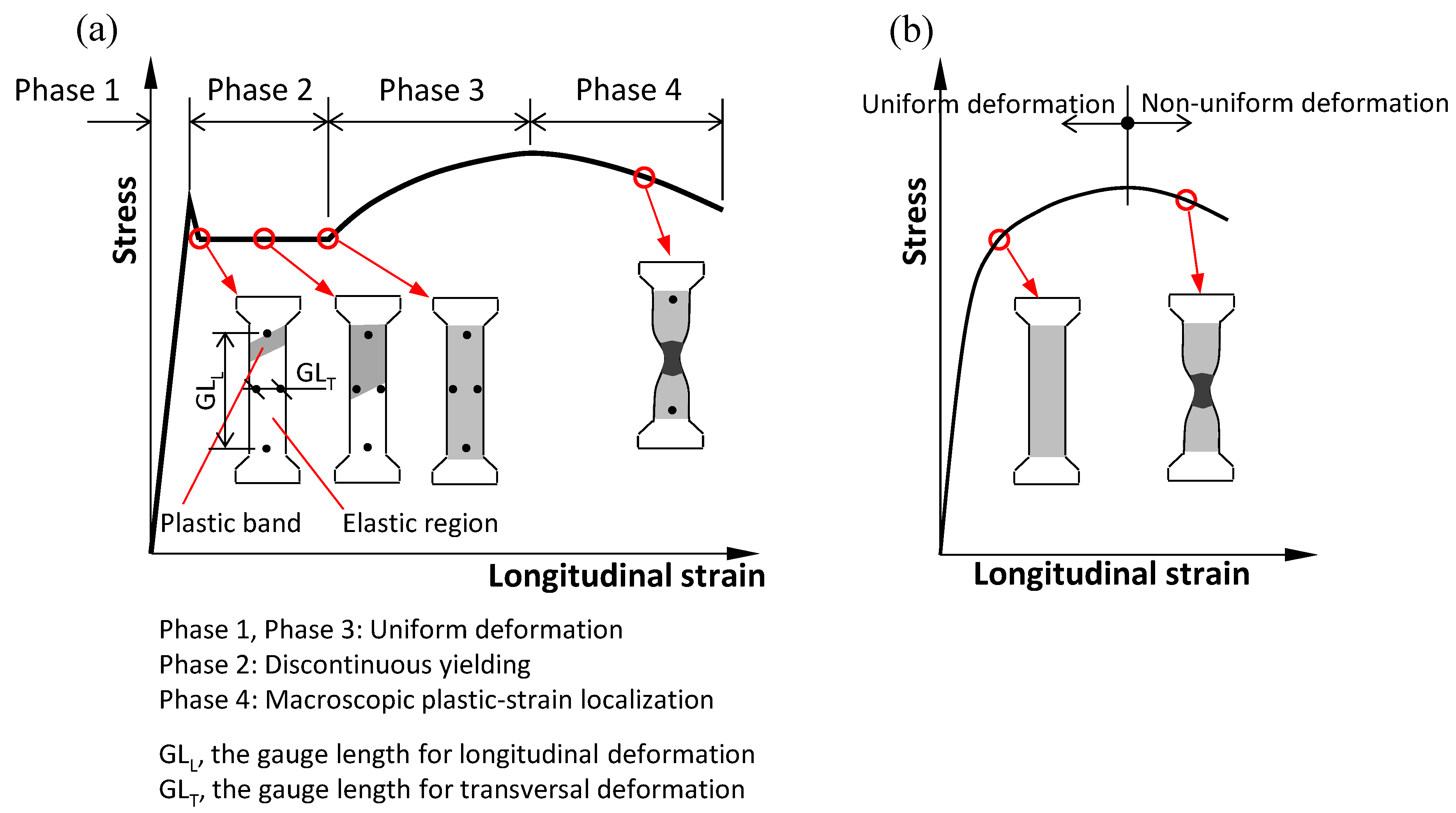
In Figure 1a, the onset point of specimen necking is a key point. On a macroscopic scale, the specimen is in a uniaxial stress state before the point, while the necked part is in a multiaxial stress state after the point. The longitudinal and transversal strains in the necked part were produced by the longitudinal and transversal stresses. According to the definition of the ν, the coefficient of the transverse strain to the longitudinal strain is not the ν. This point was not mentioned in their study.
(2)
In Phase 2, deformation is non-uniform, and thus the average ν cannot accurately represent the local value in some regions. The valid range of the average ν and the error between the average ν and the local ν need to be investigated.
(3)
A plastic band is a highly localized plastic-strain region, and it is a feature of discontinuous yielding. Its correlation with the ν was unknown.
(4)
The factors affecting the ν should be revealed.
The data on the evolution of the ν in a deformation process from the elastic strain state to the large plastic strain state is basic data, that can be used in some applications, such as the simulation of deformation processes. In the present study, we tried to obtain this basic data for low-carbon hot-rolled steel with discontinuous yielding. The three questions aforementioned ((2) to (4)) were discussed through uniaxial tension tests performed at room temperature, in which the strains were measured by an extensometer, strain gauges, and the DIC technique. The main research points are as follows: (1) The evolutions of the average and local ν were determined. The valid range of the average ν and its error relative to the local ν in the three deformation phases (Phases 1–3) were investigated. (2) The distribution of the ν within a plastic band in the discontinuous-yielding phase was measured. (3) Strain rate is a factor affecting the ν. Its correlation with the ν was revealed.

2. Materials and Methods

Commercial hot-rolled steel (SM490 steel) was used. Its chemical composition is 0.16%C, 1.46%Mn, and 0.44%Si. Its microstructure is composed of ferrite and pearlite. Dog-bone-type specimens were machined from a SM490 plate. The specimen size is shown in Figure 2a. As shown in Figure 2b, the front surface was sprayed with white and black paint to make speckles for DIC analysis, and two strain gauges (grid area: 1 mm × 1.1 mm) and an extensometer with a gauge length of 30 mm were attached to the back surface. These specimens were tensioned along the longitudinal direction (the x-axis) at room temperature and at a crosshead speed of 0.01 mm/s. The deformation process on the front surface within an area of 30 mm × 8 mm was continuously recorded with a digital camera at a time interval of 0.5 s. The digital images obtained were processed using VIC-2D software with a subset size of 9 pixel × 9 pixel (246 μm × 246 μm) and a step of 5 pixels (137 μm). In the DIC operation, the displacement uncertainty is 0.02 pixels.
Two strain gauges, an extensometer, and the DIC technique were used to measure the strains. The obtained strains are summarized as follows: (1) The longitudinal and transversal strains obtained via strain gauges on the back surface are the average strains over the area (strain gauge grid) of 1 mm × 1.1 mm. (2) The longitudinal strain on the back surface obtained via an extensometer is the average strain over the gauge length of 30 mm. (3) As shown in Figure 2b, an AB line (center line) on the front surface was drawn for the DIC data processing. Its length is almost equal to the gauge length of the extensometer used. The average values of the longitudinal and transversal strains over the AB line were taken as the average strains. Local longitudinal and transversal strains at any point on the front surface were also determined via DIC.

3. Results and Discussion

3.1. Longitudinal and Transversal Stress–Strain Curves

At an applied stress, strains were induced along the longitudinal and transversal directions. The relation of the longitudinal (or transversal) strain to the applied stress in the whole tension process was expressed via the longitudinal (or transversal) stress–strain curve. The induced strains were measured using an extensometer, strain gauges, and DIC. The corresponding stress–strain curves and the validity of the three strain measurement methods were discussed in this section.
An extensometer is a conventional tool used to measure the strain of a bulk material. It generally captures the whole response of a bulk material from zero load to complete fracture. However, its accuracy in the elastic region is not high. In contrast to the extensometer, a strain gauge can accurately measure a small strain, and it is a reliable tool to measure the deformation behavior within the elastic region. The DIC technique is relatively new, and it is usually used to measure a large strain. The longitudinal stress–strain curves, in which the average longitudinal strain ( ε av . x ) was measured via the three tools, are shown in Figure 3.
Figure 3a shows the whole deformation process from Phase 1 to Phase 4. To show the accuracy of the strain measurement, the stress–strain curve within the elastic region is enlarged in Figure 3b. It can be seen from Figure 3b that DIC has a low accuracy for a small strain, which agrees with the experimental results reported in the literature [3]. When the applied stress exceeds about 166 MPa, the difference in the elastic longitudinal strain among the three tools is very small. The strain gauge was only used in the elastic region. Figure 3a shows that DIC has almost the same accuracy as the extensometer until the occurrence of severe specimen necking.
A strain gauge and DIC were used to measure the average transversal strains. Their transversal stress–strain curves are shown in Figure 4. Apparently, the transversal strain is almost half that of the longitudinal strain. As shown in Figure 4b, DIC has low accuracy below a stress level of 301 MPa (much higher than the 166 MPa for the longitudinal strain). Therefore, the DIC data below a stress level of 301 MPa were not used to determine the Poisson’s ratio in later sections.

3.2. Poisson’s Ratio

This section focuses on two points:
(1)
The evolution of the ν in the tension process
The ν was quantitatively evaluated in terms of the average ν and the local ν, and the evolution of the ν is discussed from global and local viewpoints.
(2)
Interpretation of the characteristic of the ν
In the evolution of the ν, some features were exhibited, for example, the peak curve of the ν in the discontinuous-yielding region. The correlation of those features with the strain rate is investigated.

3.2.1. The Evolution of the Average ν in the Tension Process

The average longitudinal strain ( ε av . x ) and the average transversal strain ( ε av . y ) obtained via the strain gauges within Phase 1 (i.e., the elastic region) are shown in Figure 5. Fitting the data gives the following formula:
ε av . y = 0.2818 ε av . x
The fitting coefficient R is equal to 1. Equation (1) shows that the average Poisson’s ratio ( ν av = ε av . y / ε av . x ) in the elastic region is 0.282. The value of R indicates that the strain gauge measurement has excellent accuracy to measure the average Poisson’s ratio in the elastic region.
It is known that the shoulder of the tension specimen affects the deformation behavior around it. The AB line (cf. Figure 2b and Figure 3a) was used to determine the average value of the longitudinal and transversal strains in the DIC data processing. It should be clarified which part of the AB line was influenced by the specimen shoulder. It is recognized that the parallel part of the tension specimen should be uniformly deformed within Phase 1 and Phase 3, i.e., the local strain along the AB line should be uniform. In Figure 6, two points (W1 in Phase 3, and E1 in Phase 1) on the stress–strain curves are selected. The corresponding local longitudinal strains ( ε loc . x ) obtained via DIC along the AB line are shown in Figure 6. The local strain is almost uniform for a certain length, but both outside edges deviate because of the influence of the shoulder. If the influence of the shoulder is involved, a great error will be induced. Therefore, the CD line was taken as the effective length instead of the AB line to determine the average Poisson’s ratio ( ν av . CD ). Its length is 22.9 mm (about 80% of the length of the AB line). It is noted that the AB and CD lines in Figure 6 correspond to those in Figure 3a.
The average values of the local longitudinal strain ( ε loc . x ) and the local transversal strain ( ε loc . y ) over the CD line were taken as the average longitudinal strain ( ε av . x . CD ) and the average transversal strain ( ε av . y . CD ), respectively. The average Poisson’s ratio ( ν av . CD ) was given by ε av . y . CD / ε av . x . CD . The evolution of the ν av . CD in the deformation process is shown in Figure 7a. Since the deformation process is conventionally expressed by the stress–strain curve, the longitudinal stress–strain curve obtained with the extensometer is plotted simultaneously. To clearly show the detail of the ν av . CD , enlarged curves are shown in Figure 7b–d.
As shown in Figure 7b, in the elastic region (Phase 1), only the ν av . CD data corresponding to stress levels higher than 301 MPa were adopted. The ν av . CD varies in the range of 0.26‒0.31, and its average value is 0.297. The average Poisson’s ratio in the elastic region determined by the strain gauge is 0.282. The average Poisson’s ratios obtained using the two methods are almost the same, and their values agree with the data reported in the literature [2,4]. In Phase 2, the ν av . CD monotonously increases as the tension increases and reaches the maximum value (0.597) at the end of Phase 2 (cf. Figure 7c). Figure 7d shows that as the deformation enters into Phase 3, the ν av . CD first decreases and then remains almost the same, even if slight specimen necking takes place. As the specimen necking becomes severe, the ν av . CD decreases.

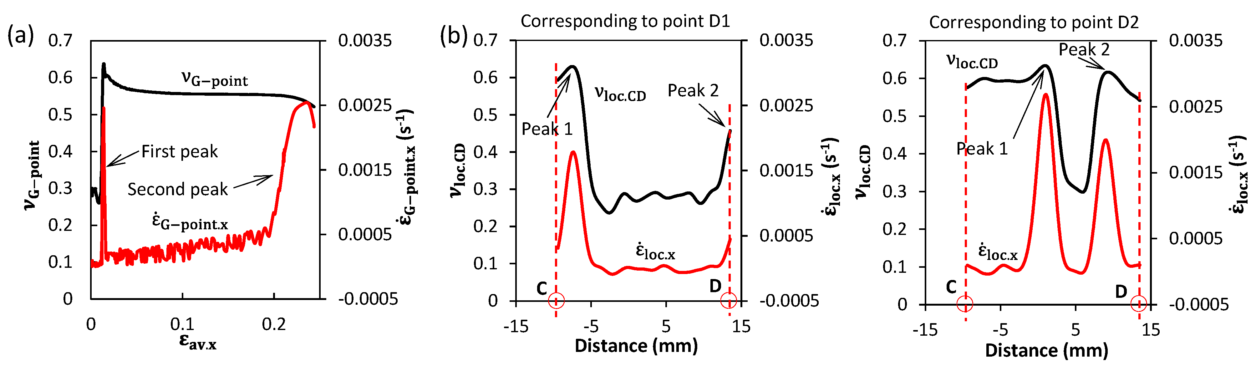
3.2.2. The Evolution of the Local Poisson’s Ratio in the Tension Process

As shown in Figure 3a, point G is on the AB line. The post-tested specimen shows that point G was in the necked region of the specimen. This means that point G experienced a complete process from the uniaxial stress state (before the onset of specimen necking) to biaxial stress state (after the onset of specimen necking). Therefore, the local Poisson’s ratio at point G ( ν G point ) was used to show the evolution of the local Poisson’s ratio in the tension process.
The evolution of the ν G point in the whole tension process is shown in Figure 7. The ν G point shows a trend similar to that of the ν av . CD , but significant differences between the average and local Poisson’s ratios in some regions are seen, for example, in Phase 2 (cf. Figure 7c).
It is believed that deformation in Phase 1 and Phase 3 is almost uniform. In Figure 6, point W1 and point E1 are in Phase 3 and Phase 1, respectively. The local Poisson’s ratio along the CD line ( ν loc . CD ) at the two stress levels is shown in Figure 8. The average Poisson’s ratio and the SD (standard deviation) are also given in Figure 8. The SD values indicate that the error at point W1 is small, and that at point E1 is allowable. Therefore, it is rational to use the average Poisson’s ratio ( ν av . CD ) to describe the local Poisson’s ratio.
Phase 2 involves the whole discontinuous-yielding process. This means that the plastic region and the elastic region exist simultaneously except at the beginning and ending points of Phase 2. In Figure 9a, two points (D1, D2) are selected. The maps of local strain rate along the x-axis (   ε   ˙ loc . x ), the local longitudinal strain ( ε loc . x ), and the local transversal strain ( ε loc . y ) corresponding to points D1 and D2 are shown in Figure 9b and c, respectively. Although band-like regions appear in the three types of maps, only the bands in the   ε   ˙ loc . x map represent the moving plastic bands [16,17]. Two plastic bands were formed. Band-1 propagates from left to right, and Band-2 goes in the opposite direction. The two bands made contact at point D2 and finally coalesced and completely disappeared at the end of Phase 2. This indicates that two plastic regions began to occur at both outside regions, extended toward the central zone (still in the elastic state), and finally merged.
The AB line and the CD line are shown in the   ε   ˙ loc . x map. The distributions of the ε loc . x and the ε loc . y along the CD line extracted from the corresponding maps are plotted in Figure 9b,c. The local Poisson’s ratio at a point on the CD line was given by ν loc . CD = ε loc . y / ε loc . x , and the distribution of the   ν loc . CD along the CD line is also given in Figure 9b,c. The plastic band width (BW) can be identified in the   ε   ˙ loc . x map. The positions of points C and D and the band width in each figure are indicated by the vertical dotted lines. In contrast to the two moving bands in Figure 9b, which have not completely merged with the CD line, they completely merged with the CD line in Figure 9c. The widths of the two moving bands at the CD line are clearly shown in Figure 9c. It can be seen that the local longitudinal and local transversal strains ( ε loc . x , ε loc . y ) and the local Poisson’s ratio ( ν loc . CD ) change significantly within the bandwidth—the ε loc . x and ε loc . y increase from an elastic strain to a very high plastic strain, and the ν loc . CD from 0.282 to 0.640. The Poisson’s ratio in the plastic region is significantly larger than that in the elastic region. The great difference in the Poisson’s ratio between the elastic region and the plastic region leads to the great error between the average Poisson’s ratio and the local Poisson’s ratio.
The experimental results obtained in this section indicate that in the elastic deformation regime and the work-hardening regime, the average Poisson’s ratio is identical to the local Poisson’s ratio, and thus the data of the Poisson’s ratio in the two regimes are basic data and can be directly used in some applications, such as calculation or simulation of the deformation process of the structural steel. However, more attention must be paid on the discontinuous-yielding regime. The elastic region and plastic region to the discontinuous-yielding regime must be separately treated by using local value instead of average value.

3.2.3. Correlation of the Poisson’s Ratio with the Strain Rate

Gere and Timoshenko [2] reported that the Poisson’s ratio of steel varies within the range of 0.27 to 0.5 from the elastic state to the complete plastic state̶in the elastic region, it is normally in the range of 0.27 to 0.30; 0.5 is a theoretical upper limit for the Poisson’s ratio of a plastic phase on the assumption that the volume of the media is constant. The present study shows that the Poisson’s ratio of the steel used is about 0.282 in the elastic region, which agrees with the data in the literature [2,4]. Its Poisson’s ratio in the plastic region is greater than 0.5. The steel used is commercial hot-rolled steel, and anisotropy of the microstructure is present. This probably makes the Poisson’s ratio of plastic phases higher than 0.5. Wojciechowski [18] established a 2D model showing that a crystalline or polycrystalline 2D system could have a Poisson’s ratio greater than 0.5.
Figure 7 shows the evolution of the average Poisson’s ratio ( ν av . CD ) over the CD line and the local Poisson’s ratio ( ν G point ) at point G in the whole tension process. When point G enters into the plastic state from the elastic state, its ν G point naturally rapidly increases. This trend agrees with the conventional understanding of Poisson’s ratio. In contrast to the previous results [3], in which the Poisson’s ratio changes slightly in the completely plastic region, a peak exists in Phase 2 (cf. Figure 7). A similar peak phenomenon was observed in the evolution of the ν av . CD . This phenomenon was not reported in the literature. Eiriksson et al. [3] investigated the Poisson’s ratio of a similar steel via DIC, but they did not find this peak phenomenon. Round bar specimens were used in their study. Because of the curvature of the specimen, the focus along the transversal direction varies, decreasing the accuracy of the speckle patterns on the digital images along the transversal direction. As a result, the error of the transversal strain obtained from these images via DIC was large. Eiriksson et al. [3] reported that the Poisson’s ratio of steel in the elastic region was 0.37, which deviates considerably from the range of 0.27 to 0.30. This experimental data verified the low measurement accuracy for the transversal strain. For this reason, their studies did not detect the peak phenomenon of the Poisson’s ratio.
The distribution of the local Poisson’s ratio ( ν loc . CD ) along the CD line is shown in Figure 9c. Two peaks (Peak 1 and Peak 2) are present. Two vertical dotted red lines are drawn from the two peak points. The cross-points of the two straight lines with the curves of the ε loc . x and the ε loc . y are the local longitudinal strain and the local transversal strain, respectively, corresponding to the two peaks. The corresponding local strains are almost half of the maximum local plastic strains. The conventional understanding is that as the local plastic strain increases, the local Poisson’s ratio increases. However, the peak phenomenon did not occur at the maximum local plastic strain, i.e., it did not agree with this conventional understanding. There must be a particular factor leading to this inconsistency.
The tension tests were performed at a constant speed, and thus it seemed that the strain rate over the specimen was almost the same in the tension process before the onset of specimen necking. However, it has been reported that when discontinuous yielding is present, the strain rate over the specimen is not uniform, and the strain rate within the moving band is much higher (almost one order) than the strain rate of the bulk material [16]. As mentioned previously, the peak phenomenon of the Poisson’s ratio is one feature of the discontinuous-yield phase (Phase 2). The correlation of this phenomenon with the strain rate is shown in Figure 10. The evolution of the local Poisson’s ratio ( ν G point ) and the local strain rate along the longitudinal direction (   ε   ˙ G point . x ) at point G during the tension process are shown in Figure 10a. In the whole tension process, the curve of the local strain rate has two peaks. The local strain-rate map showed that after the formation of a plastic band in Phase 2, the band propagated across the specimen. It is known that the plastic band is a highly strain-rate-localized region, and the maximum local strain rate within the plastic band is about ten times that in the neighboring region. The movement of the plastic band seems like the movement of a highly localized region of high strain rate, and thus when the band crossed point G, it inevitably produced a peak in the local strain rate. Point G was in the necked-specimen region. After the occurrence of specimen necking, deformation was mainly concentrated in the necked region, and other parts were hardly deformed. As a result, the localized deformation led to the second peak of the local strain rate. The first peak of the local strain rate corresponds to the peak point of the local Poisson’s ratio. The peak of the local Poisson’s ratio is apparently attributed to the high local strain rate. However, a similar correlation of the high strain rate with the local Poisson’s ratio is not seen with the second peak of the local strain rate. The two different effects of the strain rate were caused by the stress state of the specimen. For the first peak of the local strain rate, point G was in the uniaxial stress state; however, for the second peak of the local strain rate, the stress state of point G turned into a biaxial stress state due to the specimen necking. Specimen necking increased the restraint of the deformation along the transversal direction, and this effect weakened the effect of the strain rate. It is noted that because the range of the ν G point corresponding to the second peak of the local strain rate is in the necked region, the values of ( ν G point ) within the range do not represent the Poisson’s ratio.
Figure 9b,c shows that at a given stress point in Phase 2, peaks of the local Poisson’s ratio appear at certain points along the CD line. The correlation of the peak phenomenon with the strain rate is shown in Figure 10b. The fact that the peaks of the local Poisson’s ratio correspond to the peaks of strain rate indicates that a high strain rate led to the peaks of the local Poisson’s ratio. Peak 1 and Peak 2 are indicated by two arrows in Figure 10b. The local Poisson’s ratio for Peak 1 is larger than that of Peak 2. The strain rate corresponding to Peak 1 is greater than that for Peak 2. This means that the higher the strain rate is, the larger the Poisson’s ratio is.

4. Conclusions

The evolution of the Poisson’s ratio of a low-carbon hot-rolled steel in a tension process was measured using strain gauges and a digital image correlation technique. The Poisson’s ratio was evaluated in terms of the average Poisson’s ratio, which was the average value over a gauge length, and the local Poisson’s ratio at a given point. The following main results were obtained:
(1)
The distribution of the Poisson’s ratio was generally uniform in the elastic deformation regime and the hard-working regime, but it was non-uniform in the discontinuous-yielding regime. The average Poisson’s ratio was almost identical to the local Poisson’s ratio in the elastic deformation regime and the hard-working regime. In the discontinuous-yielding regime, the average Poisson’s ratio cannot accurately express the local Poisson’s ratio.
(2)
The values of the Poisson’s ratio were obtained as follows: 0.28 in the elastic regime; 0.28 to 0.64 in the discontinuous-yielding regime; and 0.55 to 0.59 in the completely plastic deformation regime.
(3)
The Poisson’s ratio changed significantly within a moving plastic band in the discontinuous-yielding phase. A high strain rate within the plastic band enhanced the Poisson’s ratio. The maximum local strain rate within the band induced the maximum local Poisson’s ratio.

Author Contributions

Conceptualization, H.Q. and T.I.; methodology, H.Q.; software, H.Q.; validation, H.Q. and T.I.; formal analysis, H.Q.; investigation, H.Q.; resources, H.Q.; data curation, H.Q. and T.I.; writing—original draft preparation, H.Q.; writing—review and editing, H.Q. and T.I.; visualization, H.Q.; supervision, H.Q. All authors have read and agreed to the published version of the manuscript.

Funding

This research received no external funding.

Data Availability Statement

Data sharing is not applicable to this article.

Conflicts of Interest

The authors declare no conflict of interest.

References

  1. Ashby, M.F.; Jones, D.R.H. Engineering Materials 1, An Introduction to Properties, Applications and Design, 3rd ed.; Elsevier Ltd: London, UK, 2005; p. 35. [Google Scholar]
  2. Gere, J.M.; Timoshenko, S.P. Mechanics of Materials, 3rd ed.; Chapman & Hall: London, UK, 1991. [Google Scholar]
  3. Eiriksson, H.J.; Bessason, B.; Unnthorsson, R. Uniaxial and lateral strain behavior of ribbed reinforcement bars inspected with digital image correlation. Struct. Concr. 2018, 19, 1992–2003. [Google Scholar] [CrossRef] [Green Version]
  4. JIMM (The Japan Institute of Materials and Metals), ISIJ (The Iron and Steel Institute of Japan). Handbook of Steels; Maruzen: Tokyo, Japan, 1967. [Google Scholar]
  5. Dmitriev, S.V.; Shigenari, T.; Abe, K. Poisson ratio beyond the limits of the elasticity theory. J. Phys. Soc. Jpn. 2001, 70, 1431–1432. [Google Scholar] [CrossRef]
  6. Zimin, B.A.; Smirnov, I.V.; Sudenkov, Y.V. Behavior of lateral-deformation coefficients during elastoplastic deformation of metals. Mechanics 2017, 62, 306–309. [Google Scholar] [CrossRef]
  7. Wang, B.R.; Sun, T.; Fezzaa, K.; Huang, J.Y.; Luo, S.N. Rate-dependent deformation and Poisson’s effect in porous titanium. Mater. Letters 2019, 245, 134–137. [Google Scholar] [CrossRef]
  8. Bhagavathula, K.B.; Meredith, C.S.; Ouellet, S.; Romanyk, D.L.; Hogan, J.D. Density, strain rate and strain effects on mechanical property evolution in polymeric foams. Int. J. Impact Eng. 2022, 161, 104100. [Google Scholar] [CrossRef]
  9. Filanova, Y.; Hauptmann, J.; Längler, F.; Naumenko, K. Inelastic behavior of polyoxymethylene for wide strain rate and temperature ranges: Constitutive modeling and identification. Materials 2021, 14, 3667. [Google Scholar] [CrossRef]
  10. Wei, Y.L.; Zao, L.Y.; Yuan, T.; Liu, W. Study on mechanical properties of shale under different loading rates. Front. Earth Sci. 2022, 9, 815616. [Google Scholar] [CrossRef]
  11. ISIJ (The Iron and Steel Institute of Japan). Handbook of Steels, I. Fundamentals, 3rd ed.; Maruzen: Tokyo, Japan, 1981. [Google Scholar]
  12. Anderson, T.L. Fracture Mechanics, Fundamentals and Applications, 3rd ed.; Taylor & Francis: London, UK, 2005. [Google Scholar]
  13. Peters, W.H.; Ranson, W.F. Digital imaging techniques in experimental stress analysis. Opt. Eng. 1982, 21, 427–431. [Google Scholar] [CrossRef]
  14. Sutton, M.A.; Wolters, W.J.; Peters, W.H.; Ranson, W.F.; McNeill, S.R. Determination of displacements using and improved digital correlation method. Image Vis. Comput. 1983, 1, 133–139. [Google Scholar] [CrossRef]
  15. Bai, R.X.; Jiang, H.; Lei, Z.K.; Liu, D.; Chen, Y.; Yan, C.; Wang, T.; Chu, Q.L. Virtual field method for identifying elastic-plastic constitutive parameters of aluminum alloy laser welding considering kinematic hardening. Opt. Lasers Eng. 2018, 110, 122–131. [Google Scholar] [CrossRef]
  16. Qiu, H.; Inoue, T.; Ueji, R. Experimental measurement of the variables of Lüders deformation in hot-rolled steel via digital image correlation. Mater. Sci. Eng. A 2020, 790, 139756. [Google Scholar] [CrossRef]
  17. Qiu, H.; Inoue, T.; Ueji, R. In-situ observation of Lüders band formation in hot-rolled steel via digital image correlation. Metals 2020, 10, 530. [Google Scholar] [CrossRef] [Green Version]
  18. Wojciechowski, K.W. Remarks on “Poisson ratio beyond the limits of the elasticity theory”. J. Phys. Soc. Jpn. 2003, 72, 1819–1820. [Google Scholar] [CrossRef]
Figure 1. Illustration of two typical deformation processes via the stress–strain curve with discontinuous yielding (a) and with continuous yielding (b).
Metals 13 00562 g001
Figure 2. (a) Specimen size; (b) front surface covered by a speckle pattern. The AB line (center line) was used in DIC data processing to determine the strain. Two strain gauges were used to measure the strains along the x-axis and the y-axis on the back surface. An extensometer was attached to the back surface along the longitudinal center line to measure the longitudinal strain.
Metals 13 00562 g002
Figure 3. (a) The curve of the stress (σ) versus the longitudinal average strain ( ε av . x ), and (b) the enlargement of (a) within Phase 1 (elastic region). The ε av . x was measured using an extensometer with a gauge length of 30 mm, DIC (over the AB line), and a strain gauge.
Metals 13 00562 g003
Figure 4. (a) The curve of the stress (σ) versus the transversal average strain ( ε av . y ), and (b) the enlargement of (a) within Phase 1 (elastic region). The ε av . y was measured using DIC (over the AB line) and a strain gauge.
Metals 13 00562 g004
Figure 5. The longitudinal average strain ( ε av . x ) versus the transversal average strain ( ε av . y ) within Phase 1. The strains were measured using strain gauges.
Metals 13 00562 g005
Figure 6. The longitudinal local strain ( ε loc . x ) distribution along the AB line shown in Figure 3a at (a) point W1 in Phase 3, and (b) point E1 in Phase 1. The effective gauge length (GL) (i.e., the length of the CD line) shown in Figure 3a is 22.9 mm.
Metals 13 00562 g006
Figure 7. (a) The evolution of the average Poisson’s ratio over the CD line (νav.CD) and the local Poisson’s ratio at point G, as shown in Figure 3a (νG-point), in the tension process (from Phase 1 to Phase 4). The tension process is expressed by the stress–strain curve (σ versus ε av . x ). (b) The enlargement of (a) within Phase 1. (c) The enlargement of (a) within Phase 2. (d) The enlargement of (a) within Phases 3 and 4.
Metals 13 00562 g007
Figure 8. The distribution of the local Poisson’s ratio (νloc.CD) along the CD line corresponding to point W1 and point E1 in Figure 6. SD, standard deviation.
Metals 13 00562 g008
Figure 9. (a) Two points of interest (D1, D2) on the stress–strain curve in Phase 2. (b,c) Maps of the local strain rate along the x-axis (   ε   ˙ loc . x ), the longitudinal local strain ( ε loc . x ), and the transversal local strain ( ε loc . y ). The ε loc . x , ε loc . y , and ν loc . CD data were extracted along the CD line from the corresponding maps; (b,c) correspond to points D1 and D2, respectively. BW, bandwidth.
Metals 13 00562 g009
Figure 10. Correlation of the Poisson’s ratio with the strain rate. (a) The evolution of the local Poisson’s ratio ( ν G point ) and the longitudinal strain rate (   ε   ˙ G point . x ) at point G in the tension process. (b) The distributions of the local Poisson’s ratio ( ν loc . CD ) and the longitudinal local strain rate (   ε   ˙ loc . x ) along the CD line at two stress points (D1 and D2) are shown in Figure 9a.
Metals 13 00562 g010
Disclaimer/Publisher’s Note: The statements, opinions and data contained in all publications are solely those of the individual author(s) and contributor(s) and not of MDPI and/or the editor(s). MDPI and/or the editor(s) disclaim responsibility for any injury to people or property resulting from any ideas, methods, instructions or products referred to in the content.

