Study on the Effects of Fluid Parameters on Erosion-Enhanced Corrosion of 90/10 Copper–Nickel Alloy Using Wire Beam Electrode

Abstract

This paper clarifies the effects of the fluid parameters of flow velocity, impact angle and sand impact frequency on the erosion-enhanced corrosion of 90/10 copper–nickel alloy by combining computational fluid dynamics (CFD) simulation, wire beam electrode (WBE) technology and electrochemical measurements. The results show that under the conditions without sand particles, erosion-enhanced corrosion is dominated by the impact angle and the flow velocity at lower (<0.860 m/s) and higher (2.370~5.644 m/s) flow velocities, respectively, while both the two fluid parameters have noticeable effects on erosion-enhanced corrosion at intermediate flow velocities (0.860~2.370 m/s). In contrast, adding sand particles corresponding to the sand impact frequency can further increase the corrosion current density without changing the effects of the flow velocity and impact angle. It demonstrates that all three fluid parameters show great effects on the erosion-enhanced corrosion of 90/10 copper–nickel alloy under conditions with sand particles.

1. Introduction

Erosion–corrosion, caused by the high-speed relative motion between metal surfaces and corrosive fluids, is one of the main reasons for premature failure of various pumps, valves, pipelines, turbines, propellers and other flow handling components in petroleum, chemistry, metallurgy, power, mining, water conservancy and transportation industries [1]. In corrosive media, the total mass loss of erosion–corrosion is usually greater than the sum of the mass loss caused by pure corrosion and pure erosion [2]. The synergism or interaction between mechanical erosion and electrochemical corrosion is generally believed to be the main reason for the enhanced erosion–corrosion damage [3,4]. It has been reported that the mass losses resulting from synergistic effects are more than half of the total erosion–corrosion mass losses of carbon steels in flowing sand-containing saline solutions [5,6,7,8]. Jones et al. [9] found that the synergism accounted for about 68% of the total erosion–corrosion damage of a hyper eutectic chromium white cast iron in 3.5 wt.% NaCl solution containing 35 wt.% silica sands. Furthermore, the contribution from synergism can be as high as 80% for erosion–corrosion of pure titanium in 3.5 wt.% NaCl solution containing 6 wt.% silica sands [10]. It is undoubted that the interaction between mechanical erosion and electrochemical corrosion plays a significant role in erosion–corrosion.

In fact, the synergism between erosion and corrosion includes erosion-enhanced corrosion and corrosion-enhanced erosion. Many researchers have made efforts to study the erosion-enhanced corrosion behaviors of metals, whilst the investigations specifically focusing on corrosion-enhanced erosion are relatively scarce, probably due to the lack of effective evaluation methods. In this situation, clarifying the mechanisms of erosion-enhanced corrosion is quite significant for understanding the synergism between erosion and corrosion. It is generally accepted that the erosion-enhanced corrosion of metals in flowing corrosive media is affected by the erosion-enhanced convection and/or impacting of solid particles. Zheng et al. [11,12] found that erosion of a carbon steel in a sand-containing solution can enhance the mass transfer of dissolved oxygen, thereby intensifying the cathodic reduction reaction, which finally accelerates corrosion. The nickel aluminum bronze was reported to be corroded more easily under erosion–corrosion conditions due to the enhanced mass transfer of both dissolved oxygen and chloride ions [13,14]. On the other hand, the passive film can be ruptured by the impact of solid particles if the impact energy exceeds a certain threshold value [15]. It results in the erosion-enhanced corrosion of passive materials, as indicated by the appearance of the anodic current peaks. It has been found that there is a positive correlation between anodic current peaks and the kinetic energy of a solid particle [16,17]. Our previous work has confirmed that erosion-enhanced corrosion caused by the rupture of passive films can be aggravated when ruptured passive films cannot be timely repaired by the repassivation process at higher flow velocities [18,19,20]. In addition to passive materials, some researchers attributed the erosion-enhanced corrosion of carbon steels and copper alloys to the removal of corrosion products caused by the impact of solid particles [21,22]. Moreover, Wood et al. [23], Nešić et al. [24], Islam et al. [25] and Stack et al. [26] also regarded the surface roughening induced by the impact of solid particles to be fully or partially responsible for erosion-enhanced corrosion. Based on the summary above, it is quite complex that erosion-induced changes in mass transfer processes, electrochemical corrosion reactions and surface films could all determine the mechanism of erosion-enhanced corrosion, depending on the specific material system.

Copper and its alloys are widely used in many fields due to their high electrical conductivity, thermal conductivity, processing formability and corrosion resistance [27]. The copper alloys, such as brass, bronze and cupronickel, used for air conditioning, heating and refrigeration, and water distribution networks usually serve in flowing corrosive media and suffer from erosion-enhanced corrosion [28,29]. Abedini et al. [30] reported that corrosion of an aluminum-brass was facilitated by increasing the jet angle, which was attributed to the higher energy transferring from impacting sands to the alloy surface at larger jet angles. Wood et al. [23,31,32,33,34] found that the nickel–aluminum bronze was more prone to corrosion under erosion conditions due to the erosion-induced acceleration of the mass transfer of dissolved oxygen and chloride ions. Compared to brass and bronze whose erosion-enhanced corrosion is relatively widely studied, few studies have focused on the erosion-enhanced corrosion of copper–nickel alloys. Of note, copper–nickel alloys have become an indispensable material in shipbuilding and marine industry due to their superior corrosion resistance, antifouling property, thermal conductivity and machinability [35,36,37]. However, erosion–corrosion is still the major threat to the safe service of the components made of copper–nickel alloys. In this situation, it deserves more effort to clarify erosion-enhanced corrosion behaviors and the corresponding mechanisms of copper–nickel alloys.

For copper–nickel alloys, the factors affecting erosion-enhanced corrosion include fluid parameters such as flow velocity, impact angle and sand impact frequency. Therefore, evaluating erosion-enhanced corrosion under different fluid conditions is of great significance for understanding the synergism. However, conventional erosion–corrosion tests can usually control one fluid parameter at a time, leading to an inefficient evaluation of erosion-enhanced corrosion. In recent years, wire beam electrode (WBE) technology has been widely used in the field of corrosion research, and its ability to test a series of experimental conditions in a single experiment has been testified for some materials and corrosion forms. For example, Zeng et al. [38,39] successfully employed WBE technology, combined with a computational fluid dynamics (CFD) simulation, to study the erosion–corrosion behavior of an X65 pipe elbow and quantified the components of erosion–corrosion rates at different positions of the elbow. Therefore, combining WBE and CFD technology should be helpful to clarify erosion-enhanced corrosion of copper–nickel alloys under various fluid conditions.

Accordingly, in this study, CFD simulation is first used to determine the fluid parameters, including flow velocity, impact angle and sand impact frequency, on the surface of each wire in a WBE made of a 90/10 copper–nickel alloy. Then, potentiodynamic polarization tests with corrosion morphology observation are performed to evaluate the erosion-enhanced corrosion of each wire in the WBE under impingement conditions. Finally, the effects of flow velocity, impact angle and sand impact frequency on the erosion-enhanced corrosion of the 90/10 copper–nickel alloy are clarified.

2. Experimental

2.1. Preparation of Wire Beam Electrode and Test Solution

A 90/10 copper–nickel alloy was used as the research material in this study, and its chemical composition, tested using an inductively coupled plasma emission spectrometer (ICAP6300, Thermo Fisher Scientific, Waltham, MA, USA), is given in

Table 1. The chemical compositions (wt.%) of the 90/10 copper–nickel alloy.

Ni	Fe	Mn	C	Pb	S	P	Cu
10.4	1.51	0.59	0.009	<0.001	0.002	0.002	Bal.

. The WBE comprised 49 (7 × 7) arrayed wires of 90/10 copper–nickel alloy with a diameter of 1.0 mm. The 49 sample wires were first welded to 49 copper wires, respectively, to ensure the electrical connection, then arrayed as 7 × 7 with an interval of 1.40 ± 0.05 mm between the adjacent wires using a plastic mold and finally embedded into epoxy resin with only the head surface of each wire exposed to the test solution, as shown in Figure 1a. In this paper, each wire in the WBE was named as “wire xy”, in which x and y are the coordinate values in the x (column)–y (line) coordinate system, as illustrated in Figure 1b. Before the experiment, the exposed working surface of WBE was mechanically ground using 120, 240, 400 and 800 grid abrasive papers in sequence, then degreased in alcohol, washed in distilled water and finally dried in air. The test medium was 1 wt.% NaCl solution without or with 0.2 wt.% silica sands. The main size of the silica sand used was approximately 100–200 μm, and the size distribution can be found in our previous work [12].

2.2. Erosion–Corrosion Tests

The home-made jet impingement apparatus, as shown in Figure 2, was employed to conduct erosion–corrosion tests, which was successfully used in our previous work [40,41]. The loop system was made of 316 L stainless steel pipes with an inner diameter of 25 mm. A nozzle with an outlet diameter of 3 mm was placed at the end of the pipe, through which the test medium with relatively high flow velocities impacted on wire 0402, as marked in Figure 1b. The nozzle-to-sample distance was kept constant at 5 mm, the nominal flow velocity at the nozzle exit was set as 5 m/s, and the impingement angle was controlled at 30°. The impingement time was 168 h (7 days), after which electrochemical measurements or corrosion morphology observation using a scanning electron microscope (FEI, Waltham, MA, USA) were conducted for each 90/10 copper–nickel alloy wire.

2.3. Electrochemical Measurements

Electrochemical measurements were conducted using a electrochemical workstation (Interface 1000, Gamry Instruments, Warminster, PA, USA) in a typical three-electrode system. Each wire in the WBE, a platinum foil with a larger surface area and a saturated calomel electrode (SCE) were used as working, counter and reference electrodes, respectively. The exposed area of each wire was 0.00785 cm². The electrodes were held steadily during the impingement to avoid unexpected disturbance. Prior to testing the potentiodynamic polarization curve of each wire, the system was stabilized for 60 s by monitoring the open circuit potential (OCP). The potentiodynamic polarization tests were conducted from −250 mV (vs. OCP) to an anodic potential higher than OCP at a sweep rate of 1 mV/s. It should be mentioned that the potentiodynamic polarization curve of each wire was recorded one by one after 168 h impingement. Only the cathodic potentiodynamic polarization was tested in this study so that the total polarization testing time (~4.5 h) can be shortened to ignore the time-induced difference among wires. In order to ensure reproducibility, potentiodynamic polarization tests were repeated using at least two identical WBEs after 168 h impingement under the same conditions.

2.4. CFD Simulation

A geometry model was first built according to the practical experiment parameters using the Ansys Workbench Geometry component. Then, the geometric model was meshed using the Ansys Workbench Meshing component. It was imported in the Ansys Workbench Fluent component for the simulation of flow domain. Figure 3 presents the 3-dimensional geometry model and the mesh details of the flow domain at the impingement angle of 30°. The scale of the flow domain was W = 100 mm, L = 100 mm and H = 100 mm, and the distance of the sample surface was 40 mm from the bottom of the flow domain. The nozzle diameter (3 mm) and the distance from the nozzle to the sample surface (5 mm) were the same as those employed in the impingement test, as provided in Section 2.2. The flow velocity at the nozzle outlet was 5 m/s, which was also the same as the experiments. The non-structured mesh was used due to the irregular shape of the flow domain. Fine grids were utilized beneath the sample surface to capture the flow characteristics precisely. The mesh-independent work was performed, and a mesh number of approximately 240,202 was finalized.

When simulating the flow pattern under impingement conditions, the methods of the volume of fluid (VOF) and limited volume code were used to solve the Reynolds-Averaged Navier–Stokes (RANS) equations of liquid–solid flow. The flow properties of solid particles were analyzed using the Euler–Lagrange equation. The liquid and solid-particle phases were set as the continuous and dispersed phases, respectively. The Euler method was utilized for the former, and the dispersed particle model (DPM) was used for the latter. The DPM model was suitable for describing the particle trajectories at low concentrations and had been used in many references [42].

The VOF model regards the fluid in the control unit as a single-phase fluid with variable density. The position and shape of the free surface can be determined by the ratio function α of the volume of fluid in the calculated grid and the volume of the grid unit. For each control unit, its continuity equation is presented below:

$$\frac{\partial {\rho }_m}{\partial t}+\frac{\partial }{\partial x_i}\left({\rho }_m{u}_i\right)=0$$

(1)

$$\frac{\partial {\alpha }_1}{\partial t}+\frac{\partial }{\partial x_i}\left({\alpha }_1{u}_i\right)=0$$

(2)

$$\frac{\partial {\alpha }_2}{\partial t}+\frac{\partial }{\partial x_i}\left({\alpha }_2{u}_i\right)=0$$

(3)

where u_i is the flow velocity component in x, y and z directions, ρ_m is the density of the flow in the grid, the subscripts 1 and 2 indicate the air phase and water phase, respectively, and α₁ and α₂ are the volume fractions of air and water, respectively. The momentum equation is shown below:

$$\frac{\partial }{\partial t}\left({\rho }_m{u}_j\right)+\frac{\partial }{\partial x_i}\left({\rho }_m{u}_j\right)=-\frac{\partial p}{\partial x_i}+\frac{\partial }{\partial x_i}[\left({\mu }_m+{\mu }_t\right)(\frac{\partial u_i}{\partial x_j}+\frac{\partial u_j}{\partial x_j})]$$

(4)

where P is the fluid pressure, μ_m is the dynamic viscosity coefficient of the grid unit (μ_m = α₁μ₁ + (1 − α₁)μ₂), and μ_t is the turbulence viscosity coefficient. In this paper, the turbulence equations were resolved using the SST k-w model. Particle motion trajectories were obtained by integrating the differential equation of particle force in a Lagrangian coordinate system. They were described using DPM, where the fluid forces acting on solid particles can be simulated as follows:

$$\frac{d{u}_p}{dt}=F_D\left(u-u_p\right)+g_x\left({\rho }_p-\rho \right)/{\rho }_p+F_x$$

(5)

where $F_D\left(u-u_p\right)$ is the unit mass resistance of the solid particle, and U and U_p are the velocities of the continuous phase and solid particles, respectively. F_D can be calculated using the following equation:

$$F_D=\frac{18\mu }{{\rho }_p{D}_p^2}\frac{C_{D}Re}{24}$$

(6)

where D_p is the diameter of the solid particle, R_e is the reference Reynolds number, ρ_P is the density of the solid particle, and C_D is the drag force, which can be calculated using the ball model. The reference Reynolds number can be defined as:

$$R_e=\frac{{\rho }_P{d}_p\left(V_p-U\right)}{\mu }$$

(7)

In Equation (5), the second part of the right side is related to gravity, and the last part is related to additional forces, including the forces caused by virtual mass forces (F_x1) and pressure gradients (F_x2). They can be described using the following equations:

$$F_{x1}=\frac{1}{2}\frac{\rho }{{\rho }_P}\frac{d}{\mathrm{dt}}\left(u-u_p\right)$$

(8)

$$F_{x2}=\frac{\rho }{{\rho }_P}{u}_p\frac{\partial u}{\partial x}$$

(9)

In addition, six mesh numbers, 260,425, 240,202, 221,207, 207,660, 186,803 and 160,042 were utilized to study the effect of meshing on the simulation results. The mass averaged velocity on wire 0402 was used to compare the simulation results, as shown in Figure 4. It can be seen that the velocity tends to be independent of the mesh number when it exceeds 221,207. Therefore, the meshing method corresponding to the mesh number 240,202 was determined and used in the following simulation.

The inlet flow velocity of 5 m/s and outlet pressure of 101,325 Pa were used for the inlet and outlet boundary conditions. A default convergence criterion in the residual of 10⁻³ was set as the basic principle. The sand particles were assumed to be ideal spherical with a diameter of 150 μm and a concentration of 0.2 wt.% at the flow rate of 0.03559 kg/s. The collision between particles was negligible due to the sparse sand impact frequency.

3. Results and Discussion

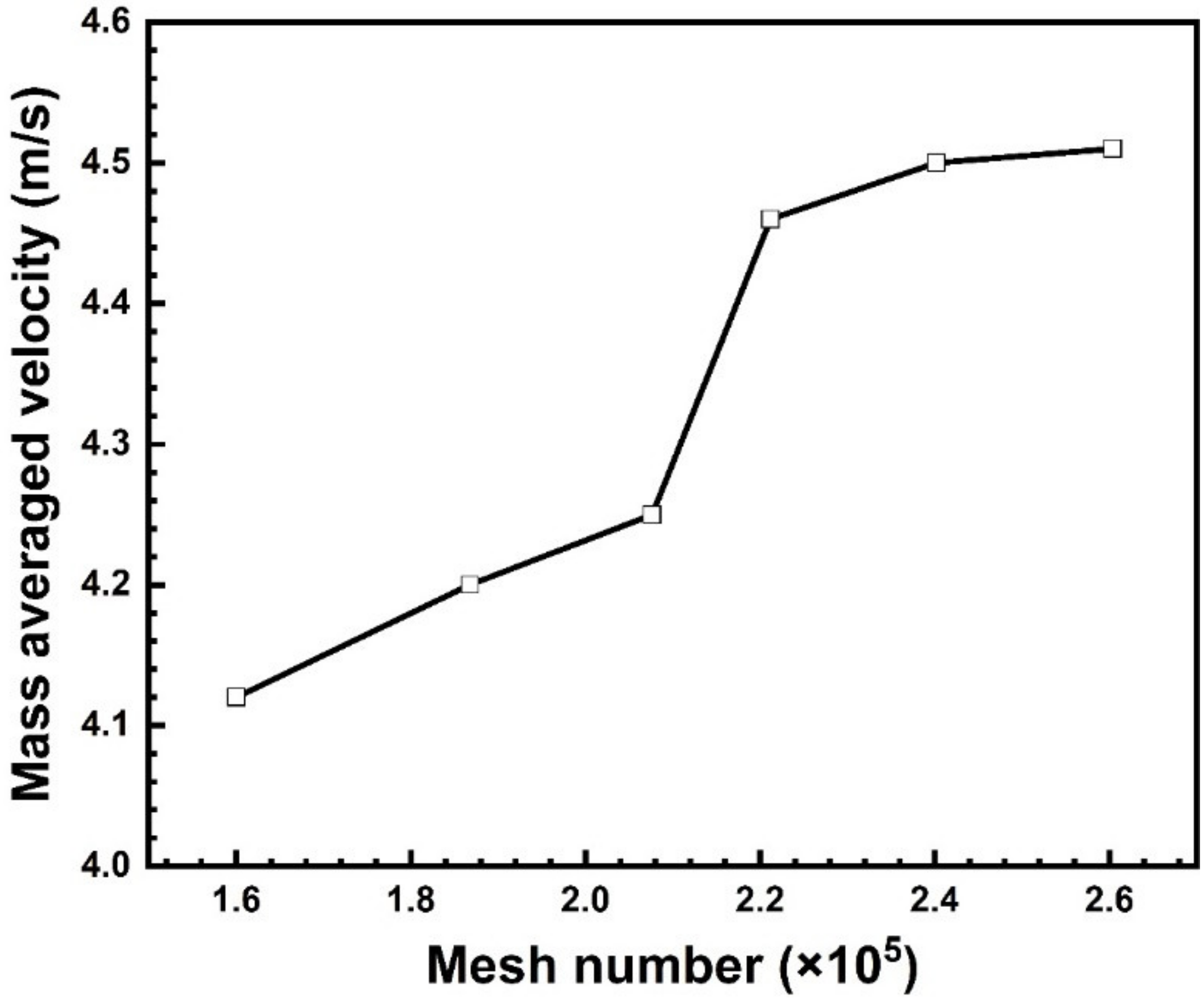
3.1. CFD Simulation

Figure 5 shows the contours of total flow velocity and sand particle trajectory along the flow direction, as well as the distribution of flow velocity and impact angle of the WBE, obtained and calculated from a CFD simulation. As seen in Figure 5a, higher flow velocities mainly focus on the wires near the impingement point, and the flow velocity decreases along the impingement direction. For the wires in the columns that are relatively far from the impingement axis (column 4), the flow velocity is lower than 0.5 m/s, which is also observed in Figure 5c. A similar phenomenon can be identified for the distribution of impact angle, as shown in Figure 5d. For the sand particle trajectory shown in Figure 5b, it can be seen that the dispersion effect of sand particles on the WBE surface is not obvious enough, and there are more sand particles only in front of the nozzle.

Figure 6a–c show the calculated total, tangential and axial flow velocities of the wire along the column of the WBE, respectively. The total flow velocity (u) and tangential flow velocity (u_t) are calculated based on the following equations:

$$u=\sqrt{u_x{}^2+u_y{}^2+u_z{}^2}$$

(10)

$$u_t=\sqrt{u_x{}^2+u_z{}^2}$$

(11)

where u_x, u_y and u_z are the flow velocity components in the x, y and z directions, which are obtained directly from the CFD simulation. It can be seen that the overall trend of total flow velocity, tangential flow velocity, axial flow velocity and impact angle is symmetrical along column 4, which means that the damaged area along the impingement direction is symmetrical. Such a phenomenon has also been found in our previous work [43]. As seen in Figure 6a, the total flow velocity of wire 0402 directly below the nozzle is the highest, reaching 5.64 m/s. For each line of the WBE, the total flow velocity shows the same decreasing trend with increasing the column number. Especially for columns 6 and 7, the total flow velocity decreases drastically to low values. In contrast, the variation trend of total flow velocity with the line number depends on the column of the WBE. In columns 4 and 5, the total flow velocity shows a generally descending trend along the impingement direction (increasing the line number from 2 to 7), while in columns 6 and 7, the variation trend with the line number is reversed. Comparing Figure 6b with Figure 6a, the variation trend of the tangential flow velocity with either the column or line numbers is basically the same as that of the total flow velocity. It could indicate that the tangential flow velocity contributes much to the total flow velocity at inclined impact angles (Figure 6d). For the axial flow velocity, as shown in Figure 6c, only its variation trend with the column number in each line resembles that of the total flow velocity, while in columns 6 and 7, it decreases to relatively low values exhibiting no noticeable difference among the lines.

Figure 6d presents the impact angle of the wire, which was calculated using the arctangent function with tangential and axial flow velocities. It can be found that the impact angle shows an upward trend with the line number, and a downward trend can be observed with the column number, except for the cases of wires 0602, 0603 and 0606 that exhibit the highest impact angles in the corresponding lines or columns. Figure 6e shows the variation of sand impact frequency obtained from the CFD simulation. Unlike the flow velocity and impact angle, not all the wires have the values of sand impact frequency, indicating that no sand particles impact on some wires. It should be attributed to the low flow velocities of these wires because higher flow velocity can bring more sand particles to impact the wire surface in the unit time. For example, the sand impact frequencies of the wires in columns 6 and 7 are almost zero, exactly corresponding to their low flow velocities (Figure 6a). Similar to the flow velocity (Figure 6a), the sand impact frequency also decreases with increasing the column number.

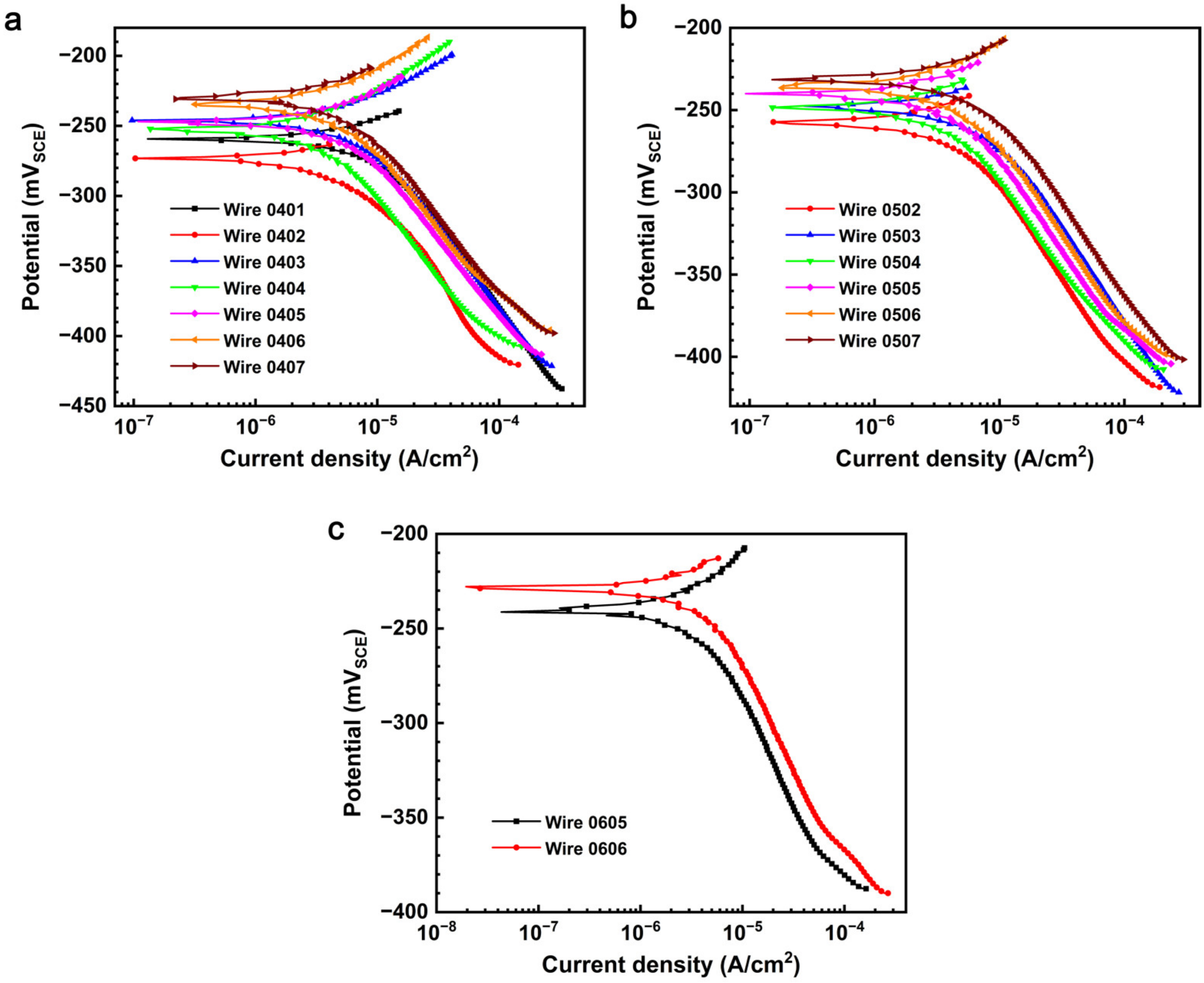
3.2. Potentiodynamic Polarization Analysis

Figure 7 shows the potentiodynamic polarization curves of the 90/10 copper–nickel alloy wires in columns 4–7 of the WBE under impingement without sand particles. Considering the symmetry of fluid parameters shown in Figure 6, only the electrochemical results of the wires in columns 4–7 are presented in this paper. In fact, the obtained corrosion current density (I_corr), representing the erosion-enhanced corrosion rate [44], of symmetrical wires is similar to each other, such as wires 0101 and 0701. As seen in Figure 7, as the line number in each column increases, the cathodic curves move to the right corresponding to the direction of higher current densities, while the evolution of the anodic curves shows a completely reversed trend. Similarly, when sand particles are added, the same evolution trend of cathodic and anodic curves with the line number can be identified, as shown in Figure 8. It should be mentioned that only potentiodynamic polarization curves of the wires with the sand impact frequency higher than zero based on the CFD simulation results (Figure 6e) are presented in Figure 8. Of note, the current fluctuation under the impingement conditions with sand particles is not noticeable compared to that without sand particles. It could be associated with the more intensive removal of corrosion products films caused by the impact of the sand particles. Furthermore, as the I_corr depends on both the anodic and cathodic portions of the potentiodynamic polarization curves, the opposite evolution of cathodic and anodic curves with the line number indicates that it is difficult to qualitatively judge the relationship of I_corr among the wires simply from the potentiodynamic polarization curves. In this situation, quantitatively Tafel fitting is needed to obtain and analyze the I_corr parameter. Herein, a cathodic Tafel fitting was employed by extending the cathodic Tafel line to the corrosion potential (E_corr) [44], and the obtained I_corr values of the wires under the impingement conditions with and without sand particles, as well as the corresponding fluid parameters, are listed in

Table 2. The obtained and calculated fluid parameters and corrosion current density of each wire in the WBE.

Wire	Total Flow Velocity (m/s)	Tangential Flow Velocity (m/s)	Axial Flow Velocity (m/s)	Impact Angle (Degree)	Sand Impact Frequency (1/s)	Icorr with Sand (μA/cm2)	Icorr without Sand (μA/cm2)
0401	5.606	5.024	2.477	26.24	309	9.242	5.147
0501	0.490	0.337	0.295	41.27	0	--	4.297
0601	0.325	0.266	0.185	34.79	0	--	3.797
0701	0.234	0.196	0.127	32.83	0	--	3.279
0402	5.644	5.421	1.553	15.98	560	10.210	5.348
0502	1.897	1.804	0.561	17.28	132	6.239	4.841
0602	0.290	0.213	0.195	42.54	0	--	4.591
0702	0.241	0.202	0.131	32.92	0	--	4.242
0403	4.615	4.539	0.812	10.15	404	7.416	4.942
0503	1.819	1.776	0.364	11.58	93	5.909	4.052
0603	0.289	0.196	0.203	46.04	0	--	3.812
0703	0.311	0.265	0.157	30.70	0	--	3.703
0404	3.565	3.528	0.478	7.71	132	5.942	4.442
0504	1.823	1.800	0.253	8.02	60	5.877	3.973
0604	0.471	0.427	0.183	23.19	0	--	3.649
0704	0.288	0.210	0.186	41.54	0	--	3.508
0405	2.370	2.350	0.258	6.27	43	5.711	4.273
0505	1.318	1.295	0.226	9.89	29	5.619	3.770
0605	0.609	0.571	0.192	18.62	1	4.583	2.826
0705	0.475	0.446	0.145	17.96	0	--	3.401
0406	1.578	1.562	0.208	7.60	25	5.424	3.949
0506	1.399	1.385	0.180	7.40	12	5.595	3.417
0606	0.860	0.839	0.171	11.50	1	4.510	2.695
0706	0.611	0.595	0.129	12.25	0	--	2.879
0407	1.536	1.525	0.169	6.32	3	5.377	3.326
0507	1.334	1.321	0.176	7.57	3	5.411	3.377
0607	1.060	1.046	0.164	8.89	0	--	2.597
0707	0.853	0.841	0.126	8.54	0	--	2.538

.

In order to show the variation of the I_corr of wires with the line and column numbers more intuitively, the I_corr value of each wire is given in the illustration of WBE, as shown in Figure 9. It can be seen that the I_corr value of wire 0402 is the largest among all the wires, regardless of the addition of sand particles. This wire is exactly the impingement point, whose flow velocity is the highest, as shown in Figure 6a. As a whole, the I_corr value decreases with increasing the line number from 2 to 7 for each column. For the wires in lines 1–4, a similar descending variation trend of I_corr with the column number is also observed, while I_corr changes irregularly for lines 5–7. The latter phenomenon could be due to the flow velocities for these wires being so low that the impact angle could become an important factor affecting I_corr. Comparing the variation trend of I_corr identified in Figure 9 with the CFD simulation results shown in Figure 6, it can be found that none of the variation trends of flow velocity, impact angle and sand impact frequency always coincide with that of I_corr. It demonstrates that the effects of fluid parameters on the erosion-enhanced corrosion of 90/10 copper–nickel alloy is quite complicated, and the dominating fluid parameters change with the impingement condition, which will be discussed in the Section 4 of this paper. Moreover, it can be also observed from Figure 9 that I_corr values under sand-containing conditions are remarkably larger than those without sand particles, especially at higher flow velocities (such as in the case of lines 1–3). Such a phenomenon can be attributed to the removal of corrosion products films induced by the impact of sand particles, which exposes the fresh surface and hence enhances corrosion.

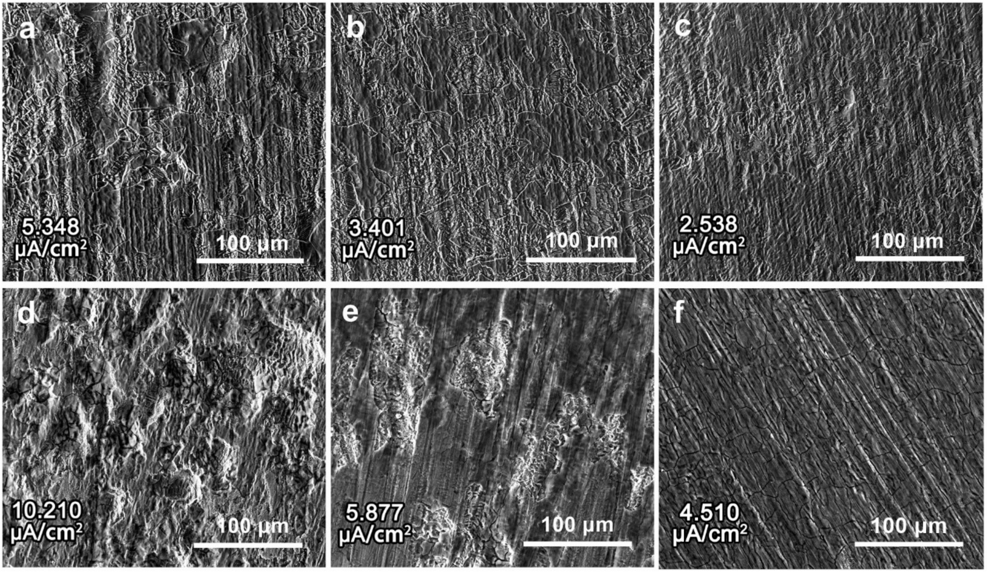
3.3. SEM Surface Characterization

Figure 10 shows the representative SEM surface morphologies of some 90/10 copper–nickel alloy wires after 168 h impingement without and with sand particles. When there are no sand particles, some corrosion pits can be observed on the surface of wire 0403 near the impingement point, whose I_corr is high compared to wire 0705 and wire 0707. In contrast, the surfaces of the latter two wires, as shown in Figure 10b,c, present the morphologies with less corrosion damage. Similarly, the corrosion is more severe as the I_corr value is increased for the cases with sand particles, as shown in Figure 10d–f. In addition, the addition of sand particles leads to more pronounced corrosion with higher I_corr values and many pits/cracks on the surface. By associating the corrosion morphology after impingement with the I_corr value, it can be found that the surface becomes more uneven with the increase of I_corr, while the lower I_corr value corresponds to a smoother surface. Accordingly, it can be confirmed that the obtained I_corr values coincide well with the observed corrosion morphology and can truly reflect the difference in the erosion-enhanced corrosion of different wires.

3.4. Effects of Fluid Parameters on Erosion-Enhanced Corrosion of 90/10 Copper–Nickel Alloy

The CFD simulation results (Figure 6) show that there are differences in the fluid parameters of flow velocity, impact angle and sand impact frequency on the surfaces of different wires in the WBE. In order to clarify the effects of these three fluid parameters on the erosion-enhanced corrosion of 90/10 copper–nickel alloy more intuitively, the variation of I_corr with the total flow velocity, tangential flow velocity, impact angle and the sand impact frequency is plotted based on the data given in Table 2, as shown in Figure 11. Overall, the I_corr exhibits a monotonous variation relation with both the flow velocity (Figure 11a,b) and sand impact frequency (Figure 11d), except for the impact angle (Figure 11c), regardless of the addition of sand particles. The irregular variation of I_corr with the impact angle could result from the irregular distribution of the impact angle on the surface of the WBE (Figure 6d). As a result, the effect of the impact angle on I_corr cannot be simply judged based on Figure 11c. Instead, it can be generally clarified by comprehensively analyzing the effects of the other two fluid parameters, which will be shown later.

It can be found from Figure 11a that the I_corr of 90/10 copper–nickel alloy under impingement with and without sand particles has almost the same variation trend with the total flow velocity. When the total flow velocity is lower than 0.860 m/s, the I_corr decreases with the flow velocity. It is noticed that the corresponding impact angle decreases gradually from 41.27 to 8.54°, and the sand impact frequency is as small as almost zero (Table 2). Many studies have shown that the erosion–corrosion rate of ductile materials increases first and then decreases with increasing the impact angle, and the maximum value appears usually at 30°~50°, due to the balance of shear and normal impact stress [7,45]. Zheng et al. [12] reported that the current density originating from erosion-enhanced corrosion changed little with the flow velocity for passive materials in liquid–solid two-phase flow media with low flow velocities and small sand impact frequencies. Accordingly, it can be considered that the decreased I_corr could result from the decreased impact angle when the total flow velocity does not exceed 0.860 m/s. In other words, the erosion-enhanced corrosion of 90/10 copper–nickel alloy is mainly dominated by the impact angle at low flow velocities (<0.860 m/s) and low sand impact frequency (almost zero).

When the total flow velocity rises to 2.370 m/s (Figure 11a), the I_corr increases as a whole but with some fluctuations, indicating the great effects of flow velocity on erosion-enhanced corrosion. Two valleys of I_corr can be identified at the flow velocities of approximately 1.5 and 1.8 m/s. Interestingly, the corresponding impact angles are smaller (<10°). Therefore, the valleys of I_corr could be attributed to the small impact angle. In this situation, it can be concluded that the erosion-enhanced corrosion of 90/10 copper–nickel alloy is primarily affected by both the flow velocity and impact angle at flow velocities lower than 2.370 m/s. Further increasing the total flow velocity to the maximum value of 5.644 m/s studied in this paper, the I_corr rises monotonously with the flow velocity, as shown in Figure 11a, while no such relationship can be found for the impact angle (Figure 11c) and sand impact frequency (Figure 11d and Table 2). A similar phenomenon has been reported in other studies [46,47], showing that the increase in flow velocity can accelerate the mass transfer and enhance the impact energy of fluids, thus aggravating erosion-enhanced corrosion damage. Accordingly, the flow velocity is the dominating fluid parameter affecting the erosion-enhanced corrosion of 90/10 copper–nickel alloy when the total flow velocity is between 2.370 and 5.644 m/s. Comparing Figure 11a,b, it can be found that the variation trend of I_corr with the total and tangential flow velocity is almost the same, demonstrating that the tangential flow velocity plays a significant role in the flow-velocity-facilitated erosion-enhanced corrosion of 90/10 copper–nickel alloy. This is because the tangential flow velocity of fluids controls the shear stress acting on the surface, which can lead to the removal or affect the formation of protective surface films and hence enhance corrosion [21,48]. Furthermore, as seen in Figure 11a–c, the addition of sand particles can increase the I_corr noticeably, i.e., accelerating erosion-enhanced corrosion. Consistently, the I_corr rises with the sand impact frequency, as shown in Figure 11d. It agrees well with the idea that the increase in sand impact frequency can enhance the impact energy of sand particles in unit time, resulting in aggravated erosion-enhanced corrosion damage [49,50]. As the sand impact frequency is almost zero when the flow velocity is lower than 0.860 m/s (Table 2), it can be concluded that, in addition to the flow velocity and impact angle, the sand impact frequency also gives rise to great effects on the erosion-enhanced corrosion of 90/10 copper–nickel alloy under the conditions with sand particles and flow velocities higher than 0.860 m/s. Based on the analysis above, it testifies that the combination of CFD simulation, WBE technology and electrochemical measurements is an effective and useful tool for clarifying the effects of various fluid parameters on the erosion-enhanced corrosion of metals.

4. Conclusions

This paper studies the effects of three fluid parameters, including flow velocity, impact angle and sand impact frequency, on the erosion-enhanced corrosion of a 90/10 copper–nickel alloy by combining CFD simulation, WBE technology and electrochemical measurements. The corrosion morphology observation confirms that the obtained corrosion current density can reflect the difference in the erosion-enhanced corrosion of different wires in the WBE. Accordingly, the following main conclusions can be made:

• For the cases without sand particles, the impact angle plays a significant role in determining the erosion-enhanced corrosion when the flow velocity is lower than 0.860 m/s. By increasing the flow velocity to 2.370 m/s, the erosion-enhanced corrosion is simultaneously controlled by the flow velocity and impact angle. When the flow velocity exceeds 2.370 m/s, the flow velocity alone becomes the dominating factor affecting erosion-enhanced corrosion. In summary, the erosion-enhanced corrosion of 90/10 copper–nickel alloy is dominated by the impact angle and flow velocity at lower and higher flow velocities, respectively.
• Adding sand particles can lead to the increase in corrosion current density, facilitating erosion-enhanced corrosion, without changing the variation trend of I_corr with the flow velocity and impact angle, when the flow velocity is higher than 0.860 m/s.
• The sand impact frequency, in addition to the flow velocity and impact angle, can also greatly accelerate the erosion-enhanced corrosion of 90/10 copper–nickel alloy.

References

1. Wang, Z.B.; Zheng, Y.G. Critical flow velocity phenomenon in erosion-corrosion of pipelines: Determination methods, mechanisms and applications. J. Pipeline Sci. Eng. 2021, 1, 63–73. [Google Scholar] [CrossRef]
2. Burstein, G.T.; Sasaki, S. Effect of impact angle on the slurry erosion–corrosion of 304L stainless steel. Wear 2000, 240, 80–94. [Google Scholar] [CrossRef]
3. Zheng, Y.G.; Yao, Z.Y.; Ke, W. Fluid mechanics factors on the corrosion mechanism of the effect of erosion. Corros. Sci. Prot. Tech. 2000, 12, 36–40. [Google Scholar]
4. Zheng, Y.G.; Yao, Z.M.; Wei, X.Y.; Ke, W. The synergistic effect between erosion and corrosion in acidic slurry medium. Wear 1995, 186, 555–561. [Google Scholar] [CrossRef]
5. Dong, H.; Qi, P.Y.; Li, X.Y.; Llewellyn, R.J. Improving the erosion–corrosion resistance of AISI 316 austenitic stainless steel by low-temperature plasma surface alloying with N and C. Mat. Sci. Eng. A-Struct. 2006, 431, 137–145. [Google Scholar] [CrossRef]
6. Elemuren, R.; Evitts, R.; Oguocha, I.; Kennell, G.; Gerspacher, R.; Odeshi, A. Slurry erosion-corrosion of 90° AISI 1018 steel elbow in saturated potash brine containing abrasive silica particles. Wear 2018, 410–411, 149–155. [Google Scholar] [CrossRef]
7. Liu, Y.; Zhao, Y.; Yao, J. Synergistic erosion–corrosion behavior of X80 pipeline steel at various impingement angles in two-phase flow impingement. Wear 2021, 466–467, 203572. [Google Scholar] [CrossRef]
8. Wen, D.-C. Erosion–corrosion behavior of plastic mold steel in solid/aqueous slurry. J. Mater. Sci. 2009, 44, 6363–6371. [Google Scholar] [CrossRef]
9. Jones, M.; Llewellyn, R.J. Erosion–corrosion assessment of materials for use in the resources industry. Wear 2009, 267, 2003–2009. [Google Scholar] [CrossRef]
10. Khayatan, N.; Ghasemi, H.M.; Abedini, M. Study of erosion–Corrosion and corrosion behavior of commercially pure-Ti during slurry erosion. J. Tribol. 2018, 140, 061609. [Google Scholar] [CrossRef]
11. Zheng, Z.B.; Zheng, Y.G. Erosion-enhanced corrosion of stainless steel and carbon steel measured electrochemically under liquid and slurry impingement. Corros. Sci. 2016, 102, 259–268. [Google Scholar] [CrossRef]
12. Zheng, Z.B.; Zheng, Y.G.; Zhou, X.; He, S.Y.; Sun, W.H.; Wang, J.Q. Determination of the critical flow velocities for erosion–corrosion of passive materials under impingement by NaCl solution containing sand. Corros. Sci. 2014, 88, 187–196. [Google Scholar] [CrossRef]
13. Wharton, J.A.; Barik, R.C.; Kear, G.; Wood, R.J.K.; Stokes, K.R.; Walsh, F.C. The corrosion of nickel–aluminium bronze in seawater. Corros. Sci. 2005, 47, 3336–3367. [Google Scholar] [CrossRef]
14. Li, L.; Qiao, Y.X.; Zhang, L.M.; Ma, A.L.; Ma, R.Y.; Zheng, Y.G. Understanding the corrosion behavior of nickel–aluminum bronze induced by cavitation corrosion using electrochemical noise: Selective phase corrosion and uniform corrosion. Materials 2023, 16, 669. [Google Scholar] [CrossRef] [PubMed]
15. Sasaki, K.; Burstein, G.T. Observation of a threshold impact energy required to cause passive film rupture during slurry erosion of stainless steel. Philos. Mag. Lett. 2000, 80, 489–493. [Google Scholar] [CrossRef]
16. Rajahram, S.S.; Harvey, T.J.; Wood, R.J.K. Electrochemical investigation of erosion–corrosion using a slurry pot erosion tester. Tribol. Int. 2011, 44, 232–240. [Google Scholar] [CrossRef]
17. Lu, B.T.; Mao, L.C.; Luo, J.L. Hydrodynamic effects on erosion-enhanced corrosion of stainless steel in aqueous slurries. Electrochim. Acta. 2010, 56, 85–92. [Google Scholar] [CrossRef]
18. Wang, Z.B.; Zheng, Y.G.; Yi, J.Z. The role of surface film on the critical flow velocity for erosion-corrosion of pure titanium. Tribol. Int. 2019, 133, 67–72. [Google Scholar] [CrossRef]
19. Li, L.L.; Wang, Z.B.; Zheng, Y.G. Interaction between pitting corrosion and critical flow velocity for erosion-corrosion of 304 stainless steel under jet slurry impingement. Corros. Sci. 2019, 158, 108084. [Google Scholar] [CrossRef]
20. Li, L.L.; Wang, Z.B.; He, S.Y.; Zheng, Y.G. Correlation between depassivation and repassivation processes determined by single particle impingement: Its crucial role in the phenomenon of critical flow velocity for erosion-corrosion. J. Mater. Sci. Technol. 2021, 89, 158–166. [Google Scholar] [CrossRef]
21. Lotz, U.; Postlethwaite, J. Erosion-corrosion in disturbed two phase liquid/particle flow. Corros. Sci. 1990, 30, 95–106. [Google Scholar] [CrossRef]
22. Zhang, G.A.; Cheng, Y.F. Electrochemical corrosion of X65 pipe steel in oil/water emulsion. Corros. Sci. 2009, 51, 901–907. [Google Scholar] [CrossRef]
23. Barik, R.C.; Wharton, J.A.; Wood, R.J.K.; Tan, K.S.; Stokes, K.R. Erosion and erosion–corrosion performance of cast and thermally sprayed nickel–aluminium bronze. Wear 2005, 259, 230–242. [Google Scholar] [CrossRef]
24. Malka, R.; Nešić, S.; Gulino, D.A. Erosion–corrosion and synergistic effects in disturbed liquid-particle flow. Wear 2007, 262, 791–799. [Google Scholar] [CrossRef]
25. Aminul Islam, M.; Farhat, Z.N.; Ahmed, E.M.; Alfantazi, A.M. Erosion enhanced corrosion and corrosion enhanced erosion of API X-70 pipeline steel. Wear 2013, 302, 1592–1601. [Google Scholar] [CrossRef]
26. Zhou, S.; Stack, M.M.; Newman, R.C. Electrochemical studies of anodic dissolution of mild steel in a carbonate-bicarbonate buffer under erosion-corrosion conditions. Corros. Sci. 1996, 38, 1071–1084. [Google Scholar] [CrossRef]
27. Francis, R. The Corrosion of Copper and Its Alloys: A Practical Guide for Engineers; Nace International: Houston, TX, USA, 2010. [Google Scholar]
28. Zhou, J.X.; Yan, L.; Tang, J.; Sun, Z.Z.; Ma, L.Q. Interactive effect of ant nest corrosion and stress corrosion on the failure of copper tubes. Eng. Failure Anal. 2018, 83, 9–16. [Google Scholar] [CrossRef]
29. Tzevelekou, T.; Flampouri, A.; Rikos, A.; Vazdirvanidis, A.; Pantazopoulos, G.; Skarmoutsos, D. Hot-water corrosion failure of a hard-drawn copper tube. Eng. Fail. Anal. 2013, 33, 176–183. [Google Scholar] [CrossRef]
30. Abedini, M.; Ghasemi, H.M. Synergistic erosion–corrosion behavior of Al–brass alloy at various impingement angles. Wear 2014, 319, 49–55. [Google Scholar] [CrossRef]
31. Barik, R.C.; Wharton, J.A.; Wood, R.J.K.; Stokes, K.R. Electro-mechanical interactions during erosion–corrosion. Wear 2009, 267, 1900–1908. [Google Scholar] [CrossRef]
32. Rajahram, S.S.; Harvey, T.J.; Wood, R.J.K. Erosion–corrosion resistance of engineering materials in various test conditions. Wear 2009, 267, 244–254. [Google Scholar] [CrossRef]
33. Rajahram, S.S.; Harvey, T.J.; Wood, R.J.K. Evaluation of a semi-empirical model in predicting erosion–Corrosion. Wear 2009, 267, 1883–1893. [Google Scholar] [CrossRef]
34. Basumatary, J.; Wood, R.J.K. Synergistic effects of cavitation erosion and corrosion for nickel aluminium bronze with oxide film in 3.5% NaCl solution. Wear 2017, 376–377, 1286–1297. [Google Scholar] [CrossRef]
35. Mansfeld, F.; Liu, G.; Xiao, H.; Tsai, C.H.; Little, B.J. The corrosion behavior of copper alloys, stainless steels and titanium in seawater. Corros. Sci. 1994, 36, 2063–2095. [Google Scholar] [CrossRef]
36. Schleich, W. Typical failures of CuNi 90/10 seawater tubing systems and how to avoid them. In Proceedings of the EUROCORR 2004, Nice, France, 12–16 September 2004. [Google Scholar]
37. Schleich, W. Application of copper-nickel alloy UNS C70600 for seawater service. In Proceedings of the CORROSION 2005, Houston, TX, USA, 3–7 April 2005. [Google Scholar]
38. Zeng, L.; Zhang, G.A.; Guo, X.P. Erosion–corrosion at different locations of X65 carbon steel elbow. Corros. Sci. 2014, 85, 318–330. [Google Scholar] [CrossRef]
39. Zeng, L.; Shuang, S.; Guo, X.P.; Zhang, G.A. Erosion-corrosion of stainless steel at different locations of a 90° elbow. Corros. Sci. 2016, 111, 72–83. [Google Scholar] [CrossRef]
40. Zheng, Z.B.; Zheng, Y.G.; Sun, W.H.; Wang, J.Q. Effect of applied potential on passivation and erosion–corrosion of a Fe-based amorphous metallic coating under slurry impingement. Corros. Sci. 2014, 82, 115–124. [Google Scholar] [CrossRef]
41. Wang, Y.; Zheng, Y.G.; Ke, W.; Sun, W.H.; Hou, W.L.; Chang, X.C.; Wang, J.Q. Slurry erosion–corrosion behaviour of high-velocity oxy-fuel (HVOF) sprayed Fe-based amorphous metallic coatings for marine pump in sand-containing NaCl solutions. Corros. Sci. 2011, 53, 3177–3185. [Google Scholar] [CrossRef]
42. Mansouri, A.; Arabnejad, H.; Shirazi, S.A.; McLaury, B.S. A combined CFD/experimental methodology for erosion prediction. Wear 2015, 332, 1090–1097. [Google Scholar] [CrossRef]
43. Yi, J.Z.; Hu, H.X.; Wang, Z.B.; Zheng, Y.G. On the critical flow velocity for erosion-corrosion in local eroded regions under liquid-solid jet impingement. Wear 2019, 422–423, 94–99. [Google Scholar] [CrossRef]
44. Wang, Z.B.; Hu, H.X.; Zheng, Y.G.; Ke, W.; Qiao, Y.X. Comparison of the corrosion behavior of pure titanium and its alloys in fluoride-containing sulfuric acid. Corros. Sci. 2016, 103, 50–65. [Google Scholar] [CrossRef]
45. Toor, I.; Irshad, H.; Badr, H.; Samad, M. The effect of impingement velocity and angle variation on the erosion corrosion performance of API 5L-X65 carbon steel in a flow loop. Metals 2018, 8, 402. [Google Scholar] [CrossRef]
46. Zeng, L.; Chen, G.; Chen, H.X. Comparative study on flow-accelerated corrosion and erosion-corrosion at a 90 degrees carbon steel bend. Materials 2020, 13, 1780. [Google Scholar] [CrossRef] [PubMed]
47. Xu, Y.Z.; Zhang, Q.L.; Zhou, Q.P.; Gao, S.; Wang, B.; Wang, X.N.; Huang, Y. Flow accelerated corrosion and erosion−Corrosion behavior of marine carbon steel in natural seawater. npj Mater. Degrad. 2021, 5, 56. [Google Scholar] [CrossRef]
48. Poulson, B. Complexities in predicting erosion corrosion. Wear 1999, 233–235, 497–504. [Google Scholar] [CrossRef]
49. Zheng, Y.G.; Yu, H.; Jiang, S.L.; Yao, Z.M. Effect of the sea mud on erosion–corrosion behaviors of carbon steel and low alloy steel in 2.4% NaCl solution. Wear 2008, 264, 1051–1058. [Google Scholar] [CrossRef]
50. Neville, A.; Reza, F.; Chiovelli, S.; Revega, T. Erosion–corrosion behaviour of WC-based MMCs in liquid–Solid slurries. Wear 2005, 259, 181–195. [Google Scholar] [CrossRef]
Figure 1. (a) Image and (b) coordinate system of wire beam electrode.
Metals 13 00380 g001
Figure 2. (a) Schematic diagram of the jet impingement apparatus for the erosion–corrosion test and (b) the enlarged sample chamber: (1) control cabinet, (2) frequency converter, (3) motor, (4) lobular pump, (5) stirring pump, (6,7) valves, (8) screw elevator, (9) thermocouple I, (10) impingement cabinet, (11) impingement angle meter, (12) electromagnetic flowmeter, (13) nozzle, (14) reference electrode, (15) counter electrode, (16) pH meter probe, (17) wire beam electrode (working electrode), (18) valve, (19) thermocouple II, (20) overflow tube, (21) slurry container, (22) cooling water, (23) heater, (24) electrochemical workstation and (25) computer.
Metals 13 00380 g002
Figure 3. (a) Three-dimensional geometry and (b) mesh details of the flow domain at the impingement angle of 30°.
Metals 13 00380 g003
Figure 4. Variation of the mass averaged velocity on wire 0402 with the mesh number.
Metals 13 00380 g004
Figure 5. (a) Contours of total flow velocity and (b) sand particle trajectory along the flow direction, and the distribution of (c) total flow velocity and (d) impact angle of the WBE obtained and calculated from CFD simulation. The dashed rectangle in (c,d) represents the location of WBE.
Metals 13 00380 g005
Figure 6. Calculated (a) total flow velocity, (b) tangential flow velocity, (c) axial flow velocity and (d) impact angle, and the obtained (e) sand impact frequency on the surface of each wire in the WBE obtained from CFD simulation.
Metals 13 00380 g006
Figure 7. Potentiodynamic polarization curves of the (a) 4th, (b) 5th, (c) 6th and (d) 7th column of 90/10 copper–nickel alloy WBE after 168 h impingement at 5 m/s using 1 wt.% NaCl solution without sand particles.
Metals 13 00380 g007
Figure 8. Potentiodynamic polarization curves of the (a) 4th, (b) 5th and (c) 6th column of 90/10 copper–nickel alloy WBE after 168 h impingement at 5 m/s using 1 wt.% NaCl solution with 0.2 wt.% sand particles.
Metals 13 00380 g008
Figure 9. Distribution of current density (unit: μA/cm2) of 90/10 copper–nickel alloy wires in the WBE after 168 h impingement at 5 m/s using 1 wt.% NaCl solution (a) without and (b) with 0.2 wt.% sand particles.
Metals 13 00380 g009
Figure 10. Representative SEM surface morphologies of some 90/10 copper–nickel alloy wires in the WBE after 168 h impingement at 5 m/s using 1 wt.% NaCl solution without sand particles: (a) wire 0403, (b) wire 0705, (c) wire 0707; and with 0.2 wt.% sand particles: (d) wire 0402, (e) wire 0504, (f) wire 0606.
Metals 13 00380 g010
Figure 11. Variation of corrosion current density (Icorr) of 90/10 copper–nickel alloy with the fluid parameters of (a) total flow velocity, (b) tangential flow velocity, (c) impact angle and (d) sand impact frequency.
Metals 13 00380 g011