Article

Phase Prediction and Visualized Design Process of High Entropy Alloys via Machine Learned Methodology

1
School of Materials Science and Engineering, Shenyang University of Technology, Shenyang 110870, China
2
Shenyang National Laboratory for Materials Science, Institute of Metal Research, CAS, Shenyang 110016, China
3
National Frontiers Science Center for Industrial Intelligence and Systems Optimization, Northeastern University, Shenyang 110819, China
*
Authors to whom correspondence should be addressed.
These authors contributed equally to this work.
Metals 2023, 13(2), 283; https://doi.org/10.3390/met13020283
Submission received: 31 December 2022 / Revised: 24 January 2023 / Accepted: 29 January 2023 / Published: 31 January 2023
(This article belongs to the Special Issue Amorphous and High-Entropy Alloy Coatings)

Abstract

:
High entropy alloys, which contain five or more elements in equal atomic concentrations, tend to exhibit remarkable mechanical and physical properties that are typically dependent on their phase constitution. In this work, a based leaner and four ensemble machine learning models are carried out to predict the phase of high entropy alloys in a database consisting of 511 labeled data. Before the models are trained, features based on the empirical design principles are selected through XGBoost, taking into account the relative importance of each feature. The ensemble learning methods of Voting and Stacking stand out among these algorithms, with a predictive accuracy of over 92%. In addition, the alloy designing process is visualized by a decision tree, introducing a new criterion for identifying phases of FCC, BCC, and FCC + BCC in high entropy alloys. These findings provide valuable information for selecting important features and suitable machine learning models in the design of high entropy alloys.

1. Introduction

Unlike traditional alloys, which are typically based on a single principal element [1,2], high-entropy alloys (HEAs) are a type of metallic alloy that consists of multiple principal elements in a single-phase solid solution, which is achieved through the maximization of configurational entropy [3]. HEAs are highly prized for their use in structural and high-temperature applications due to their mechanical properties [4], high significant refractory properties [5], high-temperature oxidation resistance [6], and excellent current sensitivity [7,8]. Based on the original HEAs design strategy, the HEAs typically adopt solid solution (SS) structures instead of complex intermetallic compounds (IM) [9]. The phase stability of HEAs can significantly impact their microstructure and, in turn, their physical and mechanical properties. For example, single phase HEAs with a face-centered cubic (FCC) structure tend to be ductile but relatively low in strength [10], while single-phase HEAs with a body-centered cubic (BCC) structure tend to exhibit high strength but are typically brittle. Dual-phase HEAs with an FCC + BCC structure can accomplish a combination of strength and ductility [11]. These three structures are the most dominant in HEAs, making the investigation of phase stability crucial for the design of new HEAs.
There have been various attempts to identify the formation of SS and IM phases in HEAs using empirical design principles, such as the entropy of mixing ( Δ S m i x ), atomic size differences ( δ ) and melting points ( T m ), electronegativity differences ( δ χ ), the enthalpy of mixing ( Δ H m i x ), and parameter Ω [12,13,14]. Although these models are able to point to certain phase formation trends, they cannot distinguish between the crystal structure of the SS phase (FCC or BCC). To address this issue, Guo et al. [15,16] proposed the empirical ( V E C ) rule based on their experimental reflection with around 20 multi-component alloys. Because very few parameters are used for fitting classification boundaries to the experimental data, these empirical criteria for a HEA composition can be easily calculated, enabling better interpretability. However, these rules are not very robust due to their reliance on the experimental data of limited composition spaces and insufficient data points [17]. Therefore, it is essential to carry out a novel and reliable first-filters for predicting phase formation tendencies in HEAs.
In recent years, ensemble algorithms [18] have shown robust vitality and excellent application prospects in guiding the phase selection in HEAs. For example, Han et al. [19] employed Extreme Gradient Boosting (XGBoost) and Random Forest to achieve higher prediction accuracy than other traditional machine learning (ML) models such as K-Nearest Neighbors, Support Vector Machine (SVM) and Decision Tree. Moreover, XGBoost and Random Forest tend to show fine and specific decision boundaries, indicating that the ensemble algorithm has a deeper understanding than the traditional ML algorithms. Beniwal et al. [20] used an averaging technique with 150 artificial neural networks to predict the phase categories, and validated their model through experimental and calculation of phase diagrams in the Al-Co-Cr-Fe-Ni, Al-Cr-Fe-Ni-Ti and Cr-Mo-V-Ni-Ti alloy system. The model-averaging technique achieves an accuracy of 91% for FCC, 97% for BCC, and 83% for IM, respectively, extending a novel strategy in exploring phase composition in HEAs.
Mishra et al. [21] proposed a stacked ensemble combining weak learners and meta-models to achieve better accuracy in classifying amorphous alloy (AM), SS, and IM phases compared to traditional SVM. Jaiswal et al. [22] used the Random Forest algorithm to achieve a test accuracy of 86% in identifying FCC, BCC, and FCC + BCC phases in HEAs. It is noteworthy that although ensemble learning methods in identifying phase in HEAs have been extensively investigated and have achieved considerably recognition, the systematic application of an ensemble strategy to distinguish between FCC, BCC, and FCC + BCC in HEAs have been largely neglected.
In this work, we collected more than 500 as-casted HEAs, including single phase FCC, single phase BCC, and dual phase FCC + BCC, to explore the formation and stability of SS phases in HEAs. Previous research in this area primarily focused on weak learners or weak learners combined with one ensemble learner. In contrast, this study systematically employed four ensemble strategies, including Bagging, Boosting, Voting, and Stacking, and also used a Decision Tree for comparison. Due to its unique algorithm principle, Decision Tree has strong interpretability and is able to visualize the classification process in a way that aligns with empirical criteria, making it particularly useful in various situations. In addition, XGBoost was used to rank the importance of features and five features were selected for further analysis. A cross-validated, receiver operating characteristic (ROC) curve and confusion matrix were employed to compare the difference and validate the effectiveness of five algorithms. Finally, we completed the decision-making process by visualizing a new phase identification path based on different ranges of alloy parameters. Overall, this study provides further insights into the design and development of HEAs.

2. Methods

2.1. Data Collection and Descriptor Construction

The experimental data of high entropy alloys (as well as a small number of medium entropy alloys) with available phase information were collected from several literatures [23,24,25,26,27,28,29,30,31]. All the alloys in our database are in the as-cast state and are quite stable solid solution alloys, including 177 single face-centered cubic (FCC) phase, 173 single body-centered cubic (BCC) phase, and 166 dual FCC and BCC phase (DP). The alloys with different solid solution phase categories are kept nearly equal in order to avoid biased prediction.
The quality of descriptors used in a machine learning (ML) model plays a crucial role in its performance. Therefore, in addition to chemical compositions, we investigated empirical design parameters involving the formation of HEA phases as an alternative approach. The formulae of these parameters are shown in Table 1, including mixing entropy ( Δ S mix ), mixing enthalpy ( Δ H mix ), melting temperature ( T m ), solid solution prediction parameter ( Ω ), valence electron concentration ( V E C ), average atom radius ( r ), atomic size difference ( δ ), electronegativity ( χ ), electronegativity difference ( Δ χ ), mean bulk modulus ( K ), standard deviation of bulk modulus ( Δ K ), mean cohesive energy ( E c o h ), and standard deviation of cohesive energy ( Δ E c o h ). In Table 1, R is the universal gas constant, c i is the atomic concentration of i t h element, n is the number of elements in the alloy, H m i x i j refers to enthalpy of mixing of the i t h and j t h elements, T m i is the melting temperature of the i t h element, V E C i is the valence electron concentration of the i t h element, χ i is the electronegativity of the i t h element, K i is the bulk modulus of the i t h element, and E c o h i refers to cohesive energy of the i t h element. Four representative entries of the dataset are shown in Table 2, describing features consisting of alloy information, 13 input features, and the classification labels.

2.2. Data Preprocessing and Features Selection

Since the features are of different units, magnitude, and range, features are normalized to make the values of all features in the same numeric weight, according to the Equation (1).
x new = x i - x ¯ σ
where x new and x i are the standardized value and the original value of the feature, respectively, and refer to the mean value and the standard deviation of each feature, respectively. The procedure guarantees all the features are evaluated equally.
Before feeding the data to the ML process, we have implemented a hybrid approach combining a correlation analysis with a wrapper method for feature selection. More concretely, the Pearson correlation was firstly employed to identify the highly correlated features. XGBoost was subsequently introduced to sieve the most important features for predicting the target property by evaluating the relative importance of each feature.
After the dataset was prepared, several models (introduced in the next section) were composed for performing machine learning. In the course of this process, original data were randomly split into two 80:20 subsets for training and testing. In addition, in the process of model training, we employ the representative 5-fold cross-validation (CV) to select the hyper-parameters of the model for stable phase prediction, so as to reduce the risk of overfitting. In order to improve prediction accuracy, each model must be trained multiple times with different hyper-parameter options.

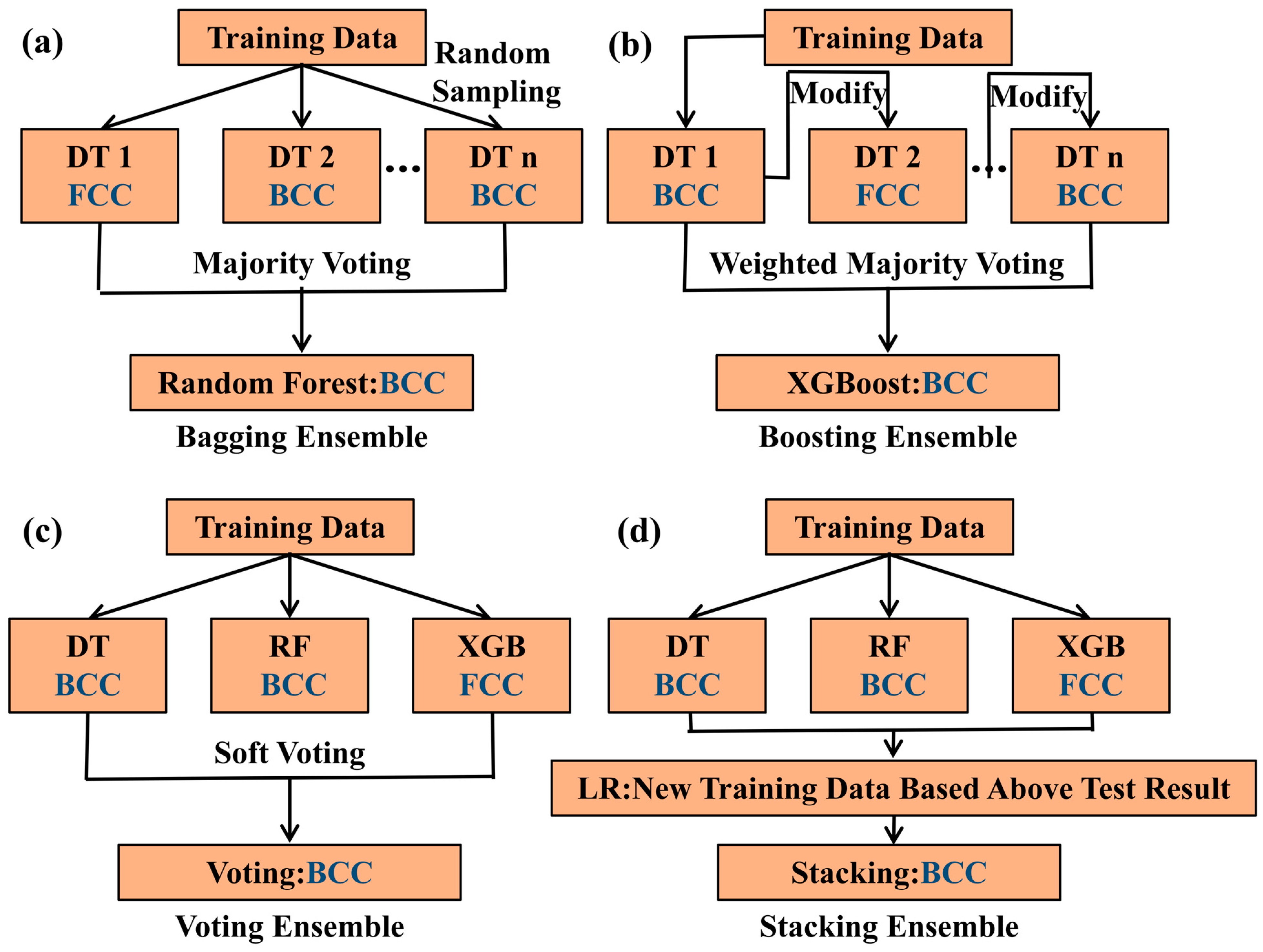
2.3. Machine Learning Algorithm

Over the last few years, various ML methods have been brought forward in different areas of research. As each ML algorithm has its own specific method of operation and potential applications, the divergence in prediction accuracy may be experienced. Following are the description of a few ML algorithms used for the present problem, including one representative supervised learning algorithm, Decision Tree, two homogeneous ensemble strategies, Bagging and Boosting, and two heterogeneous ensemble strategies, Voting and Stacking. The ML models use the Scikit-Learn open-source algorithm library [34].
The Decision Tree [35] is a supervised ML algorithm which works by creating a tree-like model of decisions based on different conditions. The tree is built by starting at the root node and then dividing the data into subsets based on the value of a feature. The process is then repeated on each subset until the leaves are pure, indicating that all the data in the leaf belongs to the same class. One advantage of decision trees is that they are easy to understand and interpret, as the tree structure clearly shows the decisions and the resulting class labels. However, decision trees can also be prone to overfitting, especially if the tree is allowed to grow too deep.
Bagging is an ensemble ML method that involves training multiple models on random subsets of the data, using the bootstrap sampling method. The final prediction is made by taking the majority vote of the individual models’ outputs. Random Forest [36] (as shown in Figure 1a), a well-known bagging algorithm, uses decision trees as its base learners and can be a good choice to reduce overfitting due to the averaging of results.
Boosting, on the other hand, involves sequentially adding new models to the ensemble, with the goal of transforming weak learners into strong ones, effectively. XGBoost [37], a common boosting method, uses gradient boosting and decision trees to create a powerful prediction model. As shown in Figure 1b, the XGBoost algorithm initially creates a model from the training dataset. Then, it builds a modified model by giving more weight to the training samples that were misclassified in the previous model. Finally, it combines all the weak models into a single, stronger model using a process called weighted majority voting.
The Voting [38] classifier is another type of ensemble method that combines the predictions of multiple models and chooses the output class with the highest probability, as determined by either a majority vote (hard voting) or an average of probabilities (soft voting), as shown in Figure 1c.
Stacking [39] is a specific type of ensemble method that involves using a higher-level model to integrate the predictions of lower-level models, in order to improve the classifier’s performance. As shown in Figure 1d, Stacking involves dividing the data into training and test sets and using a logical regression model in the second layer to combine the predictions of the first layer, which is made up of Decision Tree, Random Forest, and XGBoost models.

2.4. Evaluation Criteria of the ML Model

A confusion matrix is a basic evaluation metric of a multi-class classifier. It is presented in the form of a table and displays the number of true positive (TP), true negative (TN), false positive (FP), and false negative (FN) predictions made by the classifier. It can be useful for understanding the types of errors that the classifier is making, and for identifying any imbalances in the data. Furthermore, the accuracy score (TP + TN/(TP + FN + FP + TN)), precision score (TP/(TP + FP)), recall score (TP/(TP + FN)), precision score (TP/(TP + FP)), recall score (TP/(TP + FN)), and F1 score (2 × TR/(2TP + FP + FN)) can be calculated respectively to quantify the performance of the ML classifier.
In addition, the receiver operating characteristic (ROC) was also plotted in this work to evaluate the performance of our ML classifier. ROC is a graphical plot of the true positive rate (TPR = TP/(TP + FN)) against the false positive rate (FPR = FP/(TN + FP)) for the different possible cut-off points of a diagnostic test. The ROC curve is a useful tool for comparing the performance of different classifiers, as it is a plot of the classifier’s performance across all possible classification thresholds. The area under the ROC curve (AUC) is a measure of the classifier’s performance. An AUC of 1 indicates a perfect classifier, while an AUC of 0.5 indicates a classifier that is no better than random chance.

3. Results and Discussion

3.1. Feature Selection

To improve the robustness of our model by eliminating irrelevant features, correlations between the design features were firstly evaluated using the Pearson correlation [40], as shown in Equation (2).
r a b = 1 n 1 i = 1 n ( a i a ¯ ) ( b i b ¯ ) S a S b
where a i and b i are the sample value of the parameters, a ¯ and b ¯ are the mean value of parameters a and b , and S a and S b are the standard deviations of corresponding parameters. Correlation values range from −1 to 1, indicating considerably negative or positive relations, respectively. In Figure 2, a heat map is displayed illustrating the Pearson correlation coefficient between the 13 parameters. The matrix elements range from −0.82 to 0.97 when attaching importance to the correlation between two different features. The red-colored matrix means that the two features show a positive correlation, while blue-colored one refer to the negatively correlated features. For example, the mean bulk modulus K appears to be larger with increasing electronegativity χ , as their correlation coefficient is 0.63 (red-colored). It can be recognized that the Pearson correlation coefficient between T m and E c o h is extremely high at 0.97. The features are so correlated that the model may be prone to overfitting, making it more difficult to train the model and impact prediction accuracy [19].
It is important to consider selecting a subset of features from a high-dimensional dataset, i.e., removing redundant features during the ML process to avoid these issues [41]. XGBoost is carried out to determine the importance of the 13 features in the calculation by utilizing its feature importance analysis attribute. It should be noted that before conducting the feature importance, XGBoost was performed with default parameters to rank the importance of features objectively without any data training. Figure 3a shows the feature gain value calculated by the XGBoost model. For the importance ranking, the high-ranked descriptors consist of V E C , T m , δ K , δ , and K . According to research by Guo et al. [16], low V E C values are associated with BCC HEAs, while FCC structures tend to possess a high value of V E C . Since BCC structures typically contain refractory elements, HEAs with larger T m are more likely to have a BCC structure [5]. The parameter δ can be thought as a reflection of the atomic size misfit, with larger values potentially leading to severe lattice distortions and an increased likelihood of IM phase formation [14]. The bulk modulus, K , influences the extended atomic size misfit, which should be minimized for SS phase formation [42]. Meanwhile, this parameter standard deviation ( δ K ) has also been considered [33].
To further narrow down the descriptor space, all possible subsets of these features were considered to find the subset that resulted in the highest model accuracy. The test accuracy of the XGBoost model based on different subsets of features is plotted in Figure 3b, according to which the highest five features ( V E C , T m , δ K , δ , and K ) achieve a test accuracy of 92.16%. However, after adding the sixth most important feature E c o h (Figure 3a), the test accuracy decreases from 92.16% to 90.20%. The decreasing tendency may be caused by the high level of Pearson correlation coefficient between T m and E c o h (Figure 2), which could potentially lead to overfitting and negatively impact the test accuracy [43].
The spatial distribution of these five typical feature parameters was visualized, and statistical data analysis was conducted on the collected data to estimate the correlation among these five features, as presented in Figure 4. From the histograms, it can be seen that none of the features can be clearly separated from one another, indicating that a single feature is not sufficient to clearly distinguish the phases. It should be noted that in the BCC phase, T m appears oddly larger as V E C increases, although the Pearson correlation coefficient of V E C and T m is −0.73. Based on this plot, it can be deduced that V E C and T m are the most important features among all, which aligns with the results of the feature importance ranking by the XGBoost model. The results are similar with earlier research by Jaiswal et al. [22], showing that the parameters V E C and T m are significant for predicting phases in HEAs.

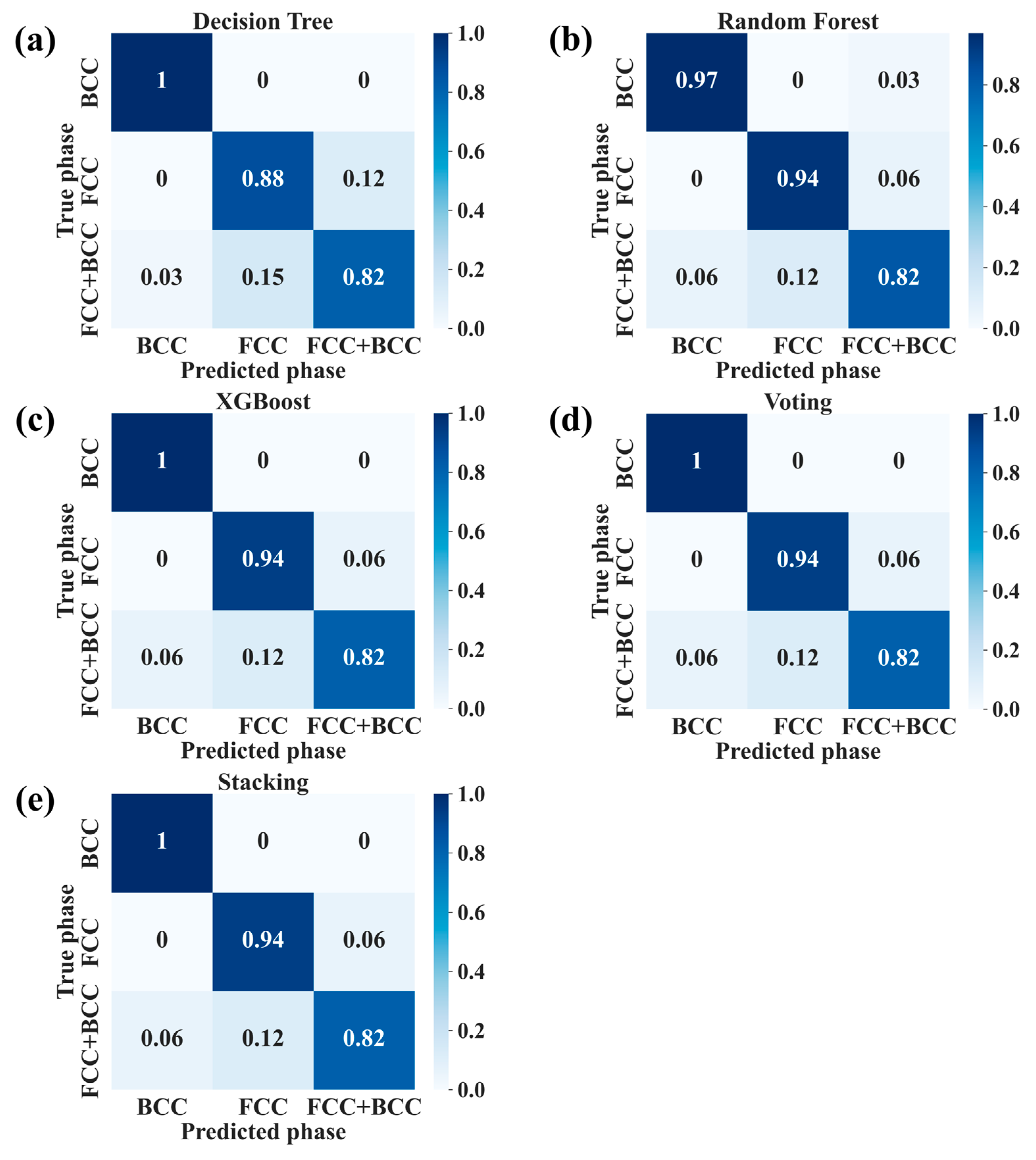
3.2. Prediction Performance of Different ML Models

These five features selected by XGBoost will be employed as input features for the training of the five ML algorithms. In addition, we use 5-fold CV to prevent overfitting in our ML models [44]. The accuracy of the CV was determined by taking the mean of the five accuracy results. The second column of Table 3 presents the mean CV accuracy and standard deviation for different algorithms, which can also be seen from the box plot in Figure 5. All the four ensemble algorithms have a mean CV accuracy of more than 85%. However, when considering the dispersion of CV accuracy, Random Forest had the lowest standard deviation of 2.50%.
After hyperparameter optimization, different measures were utilized on the test set to quantify the robustness of ML models, including accuracy, precision, recall, and F1 score. As shown in Table 3, Decision Tree has an accuracy of more than 90%, while all ensemble algorithms have an accuracy of more than 91%. Among the ensemble algorithms, XGBoost, Voting, and Stacking have the highest accuracy at 92.08%. These three algorithms also have the highest values for precision, recall, and F1 score, achieving an accuracy of 92%.
The prediction performance of the ML algorithms was validated by plotting ROC curves (Figure 6). ROC curves are utilized to emphasize the trade-off between sensitivity and specificity at different classification thresholds for a binary classifier. To extend the ROC curve to a multi-class classifier, ROC curves are drawn for each individual classification and their macro-averaged and micro-averaged forms.
Figure 6b shows that the Random Forest classification for BCC (AUC = 100.00%) and FCC (AUC = 98.00%) is slightly more reliable than for FCC + BCC (AUC = 97.00%). Both micro-averaged and macro-averaged forms have an AUC of 99.00%, which is considered satisfactory. This is similar to the findings of Riasl et al. [45], who used a Random Forest with micro-averaged and macro-averaged AUCs of 98% to create a predictive model for SS, IM, and SS + IM phases, highlighting the effectiveness of ensemble methods. Meanwhile, in common with Random Forest, Voting and Stacking also demonstrate good robustness in phase identification in HEAs and outperform other methods.
Although the ROC curve helps understand the differences between different models, it is not suitable to make a comprehensive comparison in the case of multiple classifications [45]. In such cases, a confusion matrix is often conducted to more intuitively evaluate the classification abilities of different models [44]. The performance of the ML algorithms can be analyzed by using the confusion matrix. Figure 7 depicts the confusion matrices for the testing data of 101 alloys, which consist of 34 alloys in the BCC class, 34 alloys in the FCC class, and 33 alloys in the FCC + BCC class. The five algorithms show an accuracy of over 97% for BCC, 88% for FCC, and 82% for FCC + BCC phase formation in the testing data. Decision Tree, XGBoost, and Voting and Stacking achieve a prefect accuracy of 100% for alloys with BCC phase, indicating that these algorithms are able to classify alloys in this class accurately. As for the prediction of FCC phases, the testing accuracies of four ensemble methods were 94%, while the testing accuracy of Decision Tree was 88%. This suggests that the Decision Tree is less accurate at classifying FCC alloys compared to the ensemble methods. However, all five models have an accuracy of 82% for alloys in the FCC + BCC class, which does not indicate a clear superiority of the ensemble methods over the other models in this case. Interestingly, a similar comparison was demonstrated by Jaiswal et al. [22] using Random Forest in the cases of FCC, BCC, and FCC + BCC phases, which showed that the boundary between BCC and FCC phases was clearer than that between BCC and BCC + FCC structures.
According to the analysis mentioned above, including accuracy, F1 score, recall, precision, ROC curves, and confusion matrix, all five algorithms can achieve a generous predictive accuracy, while Voting and Stacking show a better performance in identifying BCC, FCC, and FCC + BCC in HEAs.

3.3. HEAs Designing Process Visualized by Decision Tree

As discussed in Section 2, based on its unique algorithmic principles, Decision Tree has strong interpretability because it allows for the visualization of the classification process through its tree structure [19]. In this structure, each internal node represents a decision based on a feature, each branch represents a path that results from this decision, and each leaf represents the final classification outcome.
As shown in Figure 8, a three-depth tree is generated to visualize the phase designing process of HEAs. The node of tree structure is presented as a histogram, in which the abscissa of the histogram is a determined feature, and the ordinate is the number of alloys belonging to this feature. The leaf of the tree represents the phase structure and is pictured as a pie chart showing the number of alloys with predicted phases. The higher the angle of consistency with the predicted classification color, the higher the possibility of the predicted phase. According to Figure 8, the criteria identifying FCC, BCC, and FCC + BCC structure in HEAs are summarized as follow:
BCC structure in HEAs is found to be stable on the condition that V E C is between 4.18 and 6.31 with an accuracy of 100%, while V E C is between 6.31 and 7.08, K is between 139.86 and 198.31 with an accuracy of about 66.67%. FCC structure in HEAs is found to be stable, provided that the V E C is between 7.08 and 10, and δ K is between 11.78 and 29.22 with a high accuracy. The FCC structure is also stable when V E C is between 8.16 and 10, and δ K is between 29.22 and 54.58 with a high accuracy. Provided that V E C is between 6.31 and 7.08 and K is between 117.06 and 139.86, the FCC + BCC structure is steady with an accuracy of 66.67%. Meanwhile it is the FCC + BCC phase a with high accuracy when V E C is between 7.08 and 8.16, and δ K is between 29.22 and 54.58.
As shown in Figure 8, the materials descriptor, δ K , accounts for a substantial part of internal nodes in tree structure. This is consistent with result of importance ranking results in Figure 3a, which demonstrates that the V E C plays a dominant role in identifying BCC, FCC, and FCC + BCC phases in HEAs. This result aligns with the empirical criteria proposed by Guo et al. [16], which state that HEAs with V E C < 6.87, 6.87 ≤ V E C < 8 and V E C ≥ 8 are composed of BCC, BCC + FCC, and FCC phases respectively. In comparison to the empirical criteria, Decision Tree is able to visualize the classification process, including decision thresholds and more detailed paths, making it a useful tool in various situations.

4. Conclusions

In this study, ML methodology was applied to predict the formation of solid solution phases in HEAs, using an experimental database containing the phase composition and related empirical design parameters. It was revealed by the XGBoost model that the thermodynamics and atomic geometry, including the VEC, melting point, bulk modulus, atomic size difference, and standard deviation of bulk modulus, are the key features associated with the phase composition of HEAs. Subsequently, a based leaner and four ensemble machine learning models were used to predict the formation of BCC, FCC, and FCC + BCC phases in HEAs. It was found that Voting and Stacking are the most effective algorithms, with their predictive accuracy of over 92%. Additionally, a decision tree was used to visualize the alloy design process, providing a new criterion for identifying BCC, FCC, and FCC + BCC phases in HEAs.

Author Contributions

Conceptualization, S.Z.; methodology, J.G., Y.W., J.H., J.Y., K.Q., S.Z. and J.W.; investigation, J.G.; resources, J.G., Y.W., J.Y., S.Z. and J.W.; data curation, Y.W., J.H., J.Y., K.Q. and S.Z.; writing—original draft preparation, J.G. and Y.W.; writing—review and editing, Y.W., J.H. and S.Z.; project administration, S.Z. All authors have read and agreed to the published version of the manuscript.

Funding

This work was supported by the National Natural Science Foundation of China (Nos. U1908219, 52171163, 52271157, 72192830, and 72192831), the Key Research Program of the Chinese Academy of Sciences (No. ZDRW-CN-2021-2-2), the Key Research & Development Plan of Jiangxi Province (No. 20192ACB80001), the Basic scientific research project of Liaoning Province Department of Education (No. LJKZZ20220024) and the Liaoning Revitalization Talents Program (No. XLYC1907031).

Data Availability Statement

The date presented in this study are available within the article.

Conflicts of Interest

The authors declare no conflict of interest.

References

  1. Zhang, D.Y.; Qiu, D.; Fraser, H.L. Easton Additive manufacturing of ultrafine-grained high-strength titanium alloys. Nature 2019, 576, 91–95. [Google Scholar] [CrossRef] [PubMed]
  2. Wu, Z.X.; Ahmad, R.; Yin, B.; Curtin, W. Mechanistic origin and prediction of enhanced ductility in magnesium alloys. Science 2018, 359, 447–452. [Google Scholar] [CrossRef] [PubMed] [Green Version]
  3. Yeh, J.W.; Chen, S.K.; Lin, S.J.; Gan, J.Y. Nanostructured High-Entropy Alloys with Multiple Principal Element: Novel Alloy Design Concepts and Outcomes. Adv. Eng. Mater. 2004, 6, 299–303. [Google Scholar] [CrossRef]
  4. Lilensten, L.; Couzinie, J.-P. Study of a bcc multi-principal element alloy: Tensile and simple shear properties and underlying deformation mechanisms. Acta Mater. 2018, 142, 131–141. [Google Scholar] [CrossRef]
  5. Senkov, O.N.; Wilks, G.B.; Miracle, D.B. Mechanical properties of Nb25Mo25Ta25W25 and V20Nb20Mo20Ta20W20 refractory high entropy alloys. Intermetallics 2011, 19, 698–706. [Google Scholar] [CrossRef]
  6. Müller, F.; Gorr, B. On the oxidation mechanism of refractory high entropy alloys. Corros. Sci. 2019, 159, 108161. [Google Scholar] [CrossRef]
  7. Rajendrachari, S.; Adimule, V.; Gulen, M. Synthesis and Characterization of High Entropy Alloy 23Fe-21Cr-18Ni-20Ti-18Mn for Electrochemical Sensor Applications. Materials 2022, 15, 7591. [Google Scholar] [CrossRef]
  8. Rajendrachari, S. An Overview of High-Entropy Alloys Prepared by Mechanical Alloying Followed by the Characterization of Their Microstructure and Various Properties. Alloys 2022, 1, 116–132. [Google Scholar] [CrossRef]
  9. Song, H.; Tian, F.; Wang, Y. Local lattice distortion in high-entropy alloys. Phys. Rev. Mater. 2017, 1, 023404. [Google Scholar] [CrossRef] [Green Version]
  10. Senkov, O.N.; Senkova, S.V.; Woodward, C. Effect of aluminum on the microstructure and properties of two refractory high-entropy alloys. Acta Mater. 2014, 68, 214–228. [Google Scholar] [CrossRef]
  11. Zhang, Y.; Wen, C.; Su, Y.J. Phase prediction in high entropy alloys with a rational selection of materials descriptors and machine learning models. Acta Mater. 2020, 185, 528–539. [Google Scholar] [CrossRef]
  12. Zhang, Y.; Zuo, T.T.; Tang, Z.; Lu, Z.P. Microstructures and properties of high-entropy alloys. Prog. Mater. Sci. 2014, 61, 1–93. [Google Scholar] [CrossRef]
  13. Takeuchi, A.; Inoue, A. Classification of Bulk Metallic Glasses by Atomic Size Difference, Heat of mixing and period of constituent elements and its application to characterization of the main alloying element. Mater. Trans. 2005, 46, 2817–2829. [Google Scholar] [CrossRef] [Green Version]
  14. Yang, X.; Zhang, Y. Prediction of high-entropy stabilized solid-solution in multicomponent alloys. Mater. Chem. Phys. 2012, 132, 233–238. [Google Scholar] [CrossRef]
  15. Guo, S.; Liu, C.T. Phase stability in high entropy alloys: Formation of solid-solution phase or amorphous phase. Prog. Nat. Sci. Mater. Int. 2011, 21, 433–446. [Google Scholar] [CrossRef] [Green Version]
  16. Guo, S.; Liu, C.T. Effect of valence electron concentration on stability of fcc or bcc phase in high entropy alloys. J. Appl. Phys. 2011, 109, 103505. [Google Scholar] [CrossRef] [Green Version]
  17. Yang, S.G.; Lu, J.; Zhong, Y. Revisit the VEC rule in high entropy alloys (HEAs) with high-throughput CALPHAD approach and its applications for material design-A case study with AlCoCrFeNi system. Acta Mater. 2020, 192, 11–19. [Google Scholar] [CrossRef]
  18. Tang, L.X.; Meng, Y. Data analytics and optimization for smart industry. Front. Eng. Manag. 2021, 8, 157–171. [Google Scholar] [CrossRef]
  19. Han, Q.A.; Lu, Z.L.; Cui, H.T. Data-driven based phase constitution prediction in high entropy alloys. Comput. Mater. Sci. 2022, 215, 111774. [Google Scholar] [CrossRef]
  20. Beniwal, D.; Ray, P.K. Learning phase selection and assemblages in High-Entropy Alloys through a stochastic ensemble-averaging model. Comput. Mater. Sci. 2021, 197, 110647. [Google Scholar] [CrossRef]
  21. Mishra, A.; Kompella, L.; Varam, S. Ensemble-based machine learning models for phase prediction in high entropy alloys. Comput. Mater. Sci. 2022, 210, 111025. [Google Scholar] [CrossRef]
  22. Jaiswal, U.K.; Krishna, Y.V.; Phanikumar, G. Machine learning-enabled identification of new medium to high entropy alloys with solid solution phases. Comput. Mater. Sci. 2021, 197, 110623. [Google Scholar] [CrossRef]
  23. Singh, A.K.; Kumar, N.; Subramaniam, A. A geometrical parameter for the formation of disordered solid solutions in multi-component alloys. Intermetallics 2014, 53, 112–119. [Google Scholar] [CrossRef]
  24. Senkov, O.N.; Miracle, D.B. A new thermodynamic parameter to predict formation of solid solution or intermetallic phases in high entropy alloys. J. Alloy. Compd. 2016, 658, 603–607. [Google Scholar] [CrossRef] [Green Version]
  25. Couzinié, J.P.; Senkov, O.N.; Dirras, G. Comprehensive data compilation on the mechanical properties of refractory high-entropy alloys. Data Brief 2018, 21, 622–1641. [Google Scholar] [CrossRef]
  26. Chen, J.; Zhou, X.Y. A review on fundamental of high entropy alloys with promising high temperature properties. J. Alloy. Compd. 2018, 760, 15–30. [Google Scholar] [CrossRef]
  27. Gorsse, S.; Nguyen, M.H.; Miracle, D.B. Database on the mechanical properties of high entropy alloys and complex concentrated alloys. Data Brief 2018, 21, 2664–2678. [Google Scholar] [CrossRef] [PubMed]
  28. Tang, Z.W.; Zhang, S.; Wang, H.F. Designing High Entropy Alloys with Dual fcc and bcc Solid-Solution Phases: Structures and Mechanical Properties. Met. Mater. Trans. A 2019, 50, 1888–1901. [Google Scholar] [CrossRef]
  29. Senkov, O.N.; Miracle, D.B. Development and exploration of refractory high entropy alloys—A review. J. Mater. Res. 2018, 33, 3092–3128. [Google Scholar] [CrossRef] [Green Version]
  30. Ye, Y.F.; Wang, Q.; Yang, Y. High-entropy alloy: Challenges and prospects. Mater. Today 2016, 19, 349–362. [Google Scholar] [CrossRef]
  31. Tsai, M.H.; Tsai, R.C.; Huang, W.F. Intermetallic Phases in High-Entropy Alloys: Statistical Analysis of their Prevalence and Structural Inheritance. Metals 2019, 9, 247. [Google Scholar] [CrossRef] [Green Version]
  32. Zhang, Y.; Zhou, Y.J.; Lin, J.P. Solid-Solution Phase Formation Rules for Multi-component Alloys. Adv. Eng. Mater. 2008, 10, 534–538. [Google Scholar] [CrossRef]
  33. Zhou, Z.; Zhou, Y.; He, Q.; Ding, Z.; Li, F.; Yang, Y. Machine learning guided appraisal and exploration of phase design for high entropy alloys. Npj Comput. Mater. 2019, 5, 128. [Google Scholar] [CrossRef] [Green Version]
  34. Pedregosa, F.; Varoquaux, G.; Gramfort, A. Scikit-learn: Machine learning in python. J. Mach. Learn. Res. 2011, 12, 2825–2830. [Google Scholar] [CrossRef]
  35. Moshkov, M. Decision trees for regular factorial languages. Array 2022, 15, 203. [Google Scholar] [CrossRef]
  36. Breiman, L. Random Forests. Mach. Learn. 2001, 45, 5–32. [Google Scholar] [CrossRef] [Green Version]
  37. Chen, T.Q.; Cuestrin, C. XGBoost: A Scalable Tree Boosting System. In Proceedings of the 22nd ACM Sigkdd International Conference on Knowledge Discovery and Data Mining, San Francisco, CA, USA, 13–17 August 2016; pp. 785–794. [Google Scholar] [CrossRef] [Green Version]
  38. Gao, J.W.; Lin, Z.P. Voting based extreme learning machine. Inf. Sci. 2012, 185, 66–77. [Google Scholar] [CrossRef]
  39. Zenko, B.; Dzeroski, S. Stacking with an Extended Set of Meta-Level Attributes and MLR. In Machine Learning: ECML 2002; Springer: Berlin/Heidelberg, Germany, 2002; pp. 493–504. [Google Scholar] [CrossRef] [Green Version]
  40. Roy, A.; Babuska, T.; Krick, B. Machine learned feature identification for predicting phase and Young’s modulus of low-, medium- and high-entropy alloys. Scr. Mater. 2020, 185, 152–158. [Google Scholar] [CrossRef]
  41. Mangal, A.; Holm, E.A. A comparative study of feature selection methods for stress hotspot classifification in materials. Integr. Mater. Manuf. Innov. 2018, 7, 87–95. [Google Scholar] [CrossRef] [Green Version]
  42. He, Q.F.; Ye, Y.F.; Yang, Y. The configurational entropy of mixing of metastable random solid solution in complex multi-component alloys. J. Appl. Phys. 2016, 120, 154902. [Google Scholar] [CrossRef]
  43. Hawkins, D.M. The problem of overfitting. J. Chem. Inf. Comput. Sci. 2004, 44, 1–12. [Google Scholar] [CrossRef] [PubMed]
  44. Islam, N.; Huang, W.J.; Zhuang, H.L. Machine learning for phase selection in multi-principal element alloys. Comput. Mater. Sci. 2018, 150, 230–235. [Google Scholar] [CrossRef]
  45. Risal, S.; Zhu, W.H.; Guillen, P.; Sun, L. Improving phase prediction accuracy for high entropy alloys with Machine learning. Comput. Mater. Sci. 2021, 192, 110389. [Google Scholar] [CrossRef]
Figure 1. (a) Working principle of Random Forest algorithm, (b) working principle of XGBoost algorithm, (c) working principle of Voting algorithm, and (d) working principle of Stacking algorithm.
Metals 13 00283 g001
Figure 2. Heat map of inter-feature correlation by correlation analysis.
Metals 13 00283 g002
Figure 3. (a) Feature importance using the XGBoost algorithm, (b) the number of features vs. test accuracy based on XGBoost algorithm.
Metals 13 00283 g003
Figure 4. Scatter plot of the features for three phases. Scatter plots show the distributions of the three phases as a function of a pair of the 5 features. Histograms present the distributions of the three phases at different values of one of the 5 features. Different colors indicate different phases. Blue is for FCC, green for BCC, and orange refers to FCC + BCC.
Metals 13 00283 g004
Figure 5. Box plots of mean CV accuracies for five models. (The black line in the middle of the box plots indicates the mean CV accuracy of each model, and the upper and lower limits denote the maximum and minimum CV accuracies).
Metals 13 00283 g005
Figure 6. Visualization metrics for the 5 classifiers: (a) ROC-curve of Decision Tree, (b) ROC-curve of Random Forest, (c) ROC-curve of XGBoost, (d) ROC-curve of Voting, and (e) ROC-curve of Stacking.
Metals 13 00283 g006
Figure 7. Confusion matrix for training and testing of current data set using (a) Decision Tree, (b) Random Forest, (c) XGBoost, (d) Voting, and (e) Stacking. (Y axis is true phases and X axis is predicted phases for all matrices).
Metals 13 00283 g007
Figure 8. Visualize the decision-making process of the Decision Tree in test set.
Metals 13 00283 g008
Table 1. Feature list of the phase prediction model of HEA.
FormulaDefinitionReference
Δ S mix = R i = 1 n c i ln c i Mixing entropy[32]
Δ H mix = i = 1 , i < j n 4 H m i x i j c i c j Mixing enthalpy[32]
T m = i = 1 n c i T m i Melting point[14]
Ω = T m Δ S m i x / Δ H m i x Parameter for predicting the SS formation[14]
V E C = i = 1 n c i V E C i Valence electron concentration[16]
r = i = 1 n c i r i Average atom radius[32]
δ = 100 × i = 1 n c i ( 1 r i / r ) 2 Atom radius difference[32]
χ = i = 1 n c i χ i Electronegativity[11]
Δ χ = i = 1 n c i ( χ i χ ) 2 Standard deviation of electronegativity[11]
K = i = 1 n c i K i Mean bulk modulus[33]
Δ K = i = 1 n c i ( K i K ) 2 Standard deviation of bulk modulus[19]
E c o h = i = 1 n c i E c o h i Mean cohesive energy[33]
Δ E c o h = i = 1 n c i ( E c o h i E c o h ) 2 Standard deviation of cohesive energy[20]
Table 2. Four representative entries of the dataset after standardization. Each entry has eight input features.
Alloy
(Phase)
AlCuCoCNi
(FCC + BCC)
HfNbTTiZr
(BCC)
MoNbTaW
(BCC)
CoCrMnNi
(FCC)
Δ S mix ( J K 1 m o l 1 ) 13.3813.3811.5311.53
Δ H mix ( K J m o l 1 ) −6.562.72−6.5−5.5
T m ( K ) 1583251331451786
Ω 3.2312.365.583.74
V E C 7.84.45.38
r 0.130.150.140.13
δ 0.05520.04980.02320.0345
χ 1.791.451.911.75
Δ χ 0.130.120.360.15
K 147.2135.4200160
Δ K 38.5742.4321.2124.49
E c o h 381.6638.2749384
Δ E c o h 43.6856.4954.7439.19
Table 3. Best performance of different machine learning algorithms on the dataset.
AlgorithmsMean CV
Accuracy (%)
Accuracy (%)Precision (%)Recall (%)F1 Score (%)
Decision
Tree
83.76 (±3.35)90.10909090
Random
Forest
87.13 (±2.50)91.09919191
XGBoost86.93 (±4.03)92.08929292
Voting86.73 (±2.84)92.08929292
Stacking86.53 (±2.77)92.08929292
Disclaimer/Publisher’s Note: The statements, opinions and data contained in all publications are solely those of the individual author(s) and contributor(s) and not of MDPI and/or the editor(s). MDPI and/or the editor(s) disclaim responsibility for any injury to people or property resulting from any ideas, methods, instructions or products referred to in the content.

