
Numerical Simulation of Bubble Size Distribution in Single Snorkel Furnace (SSF) with Population Balance Model (PBM)


Abstract
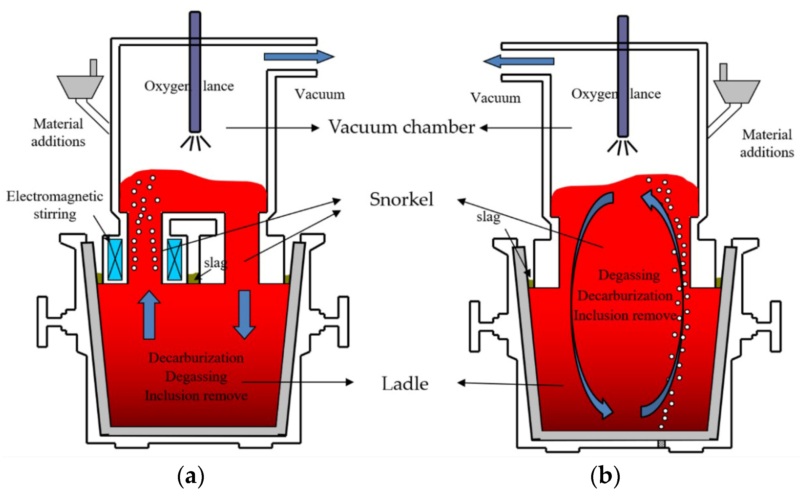
:1. Introduction
1.1. Previous Works in Flow Structures and Decarbonization Modelling
1.2. Significance of Bubble Dynamics and Its Impact on Decarburization
2. Mathematical Modeling
2.1. Euler–Euler Two-Fluid Model
2.2. Momentum Transfer
2.2.1. Drag Force
2.2.2. Lift Force
2.2.3. Virtual Mass Force
2.3. User-Defined Scalar (UDS) Transport Equations
2.4. Population Balance Model (PBM) for Bubble Dynamics
2.4.1. Breakage
2.4.2. Coalescence
2.5. Numerical Details
3. Results and Discussion
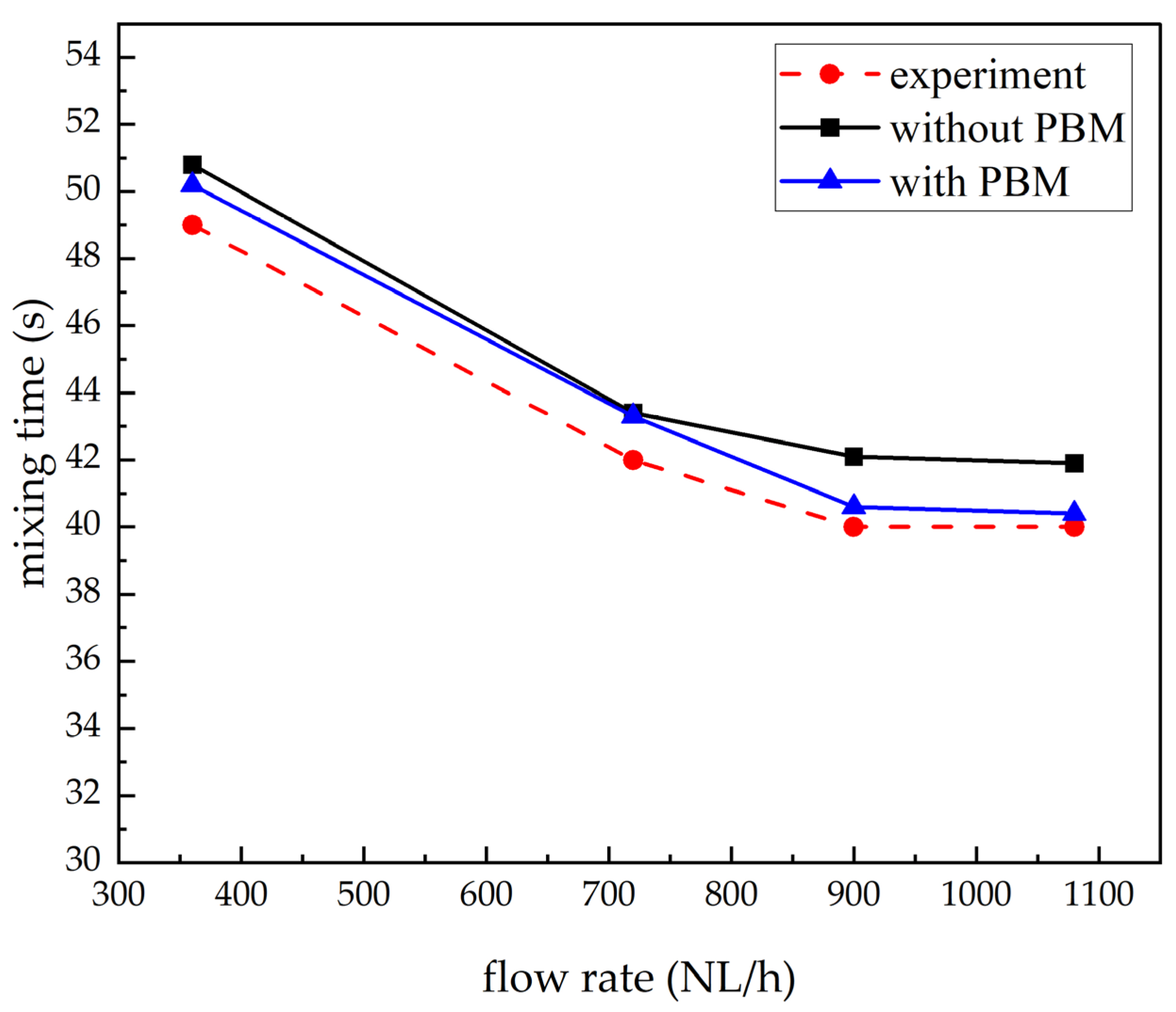
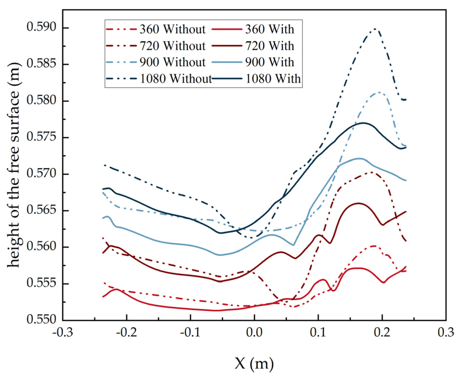
3.1. Validation of Numerical Model
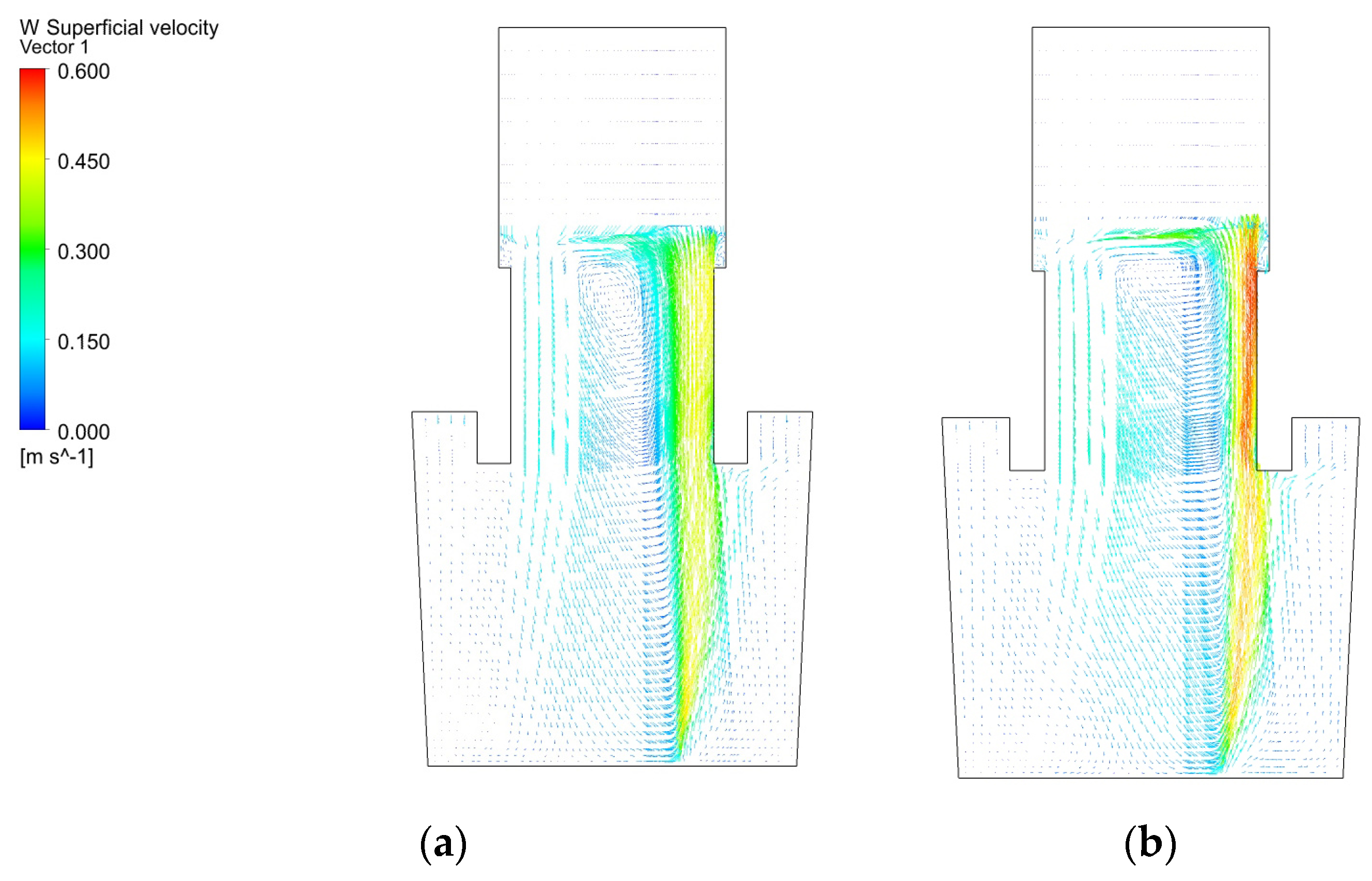
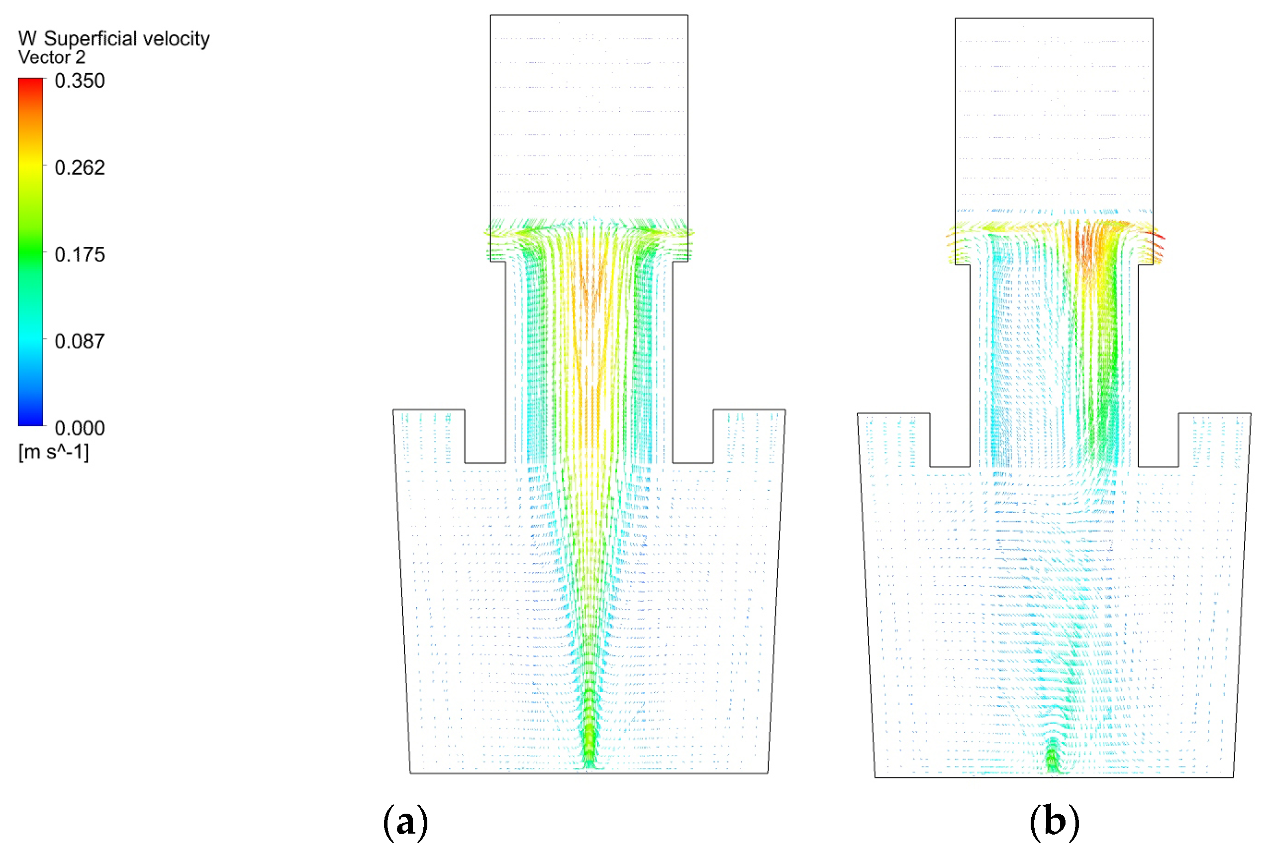
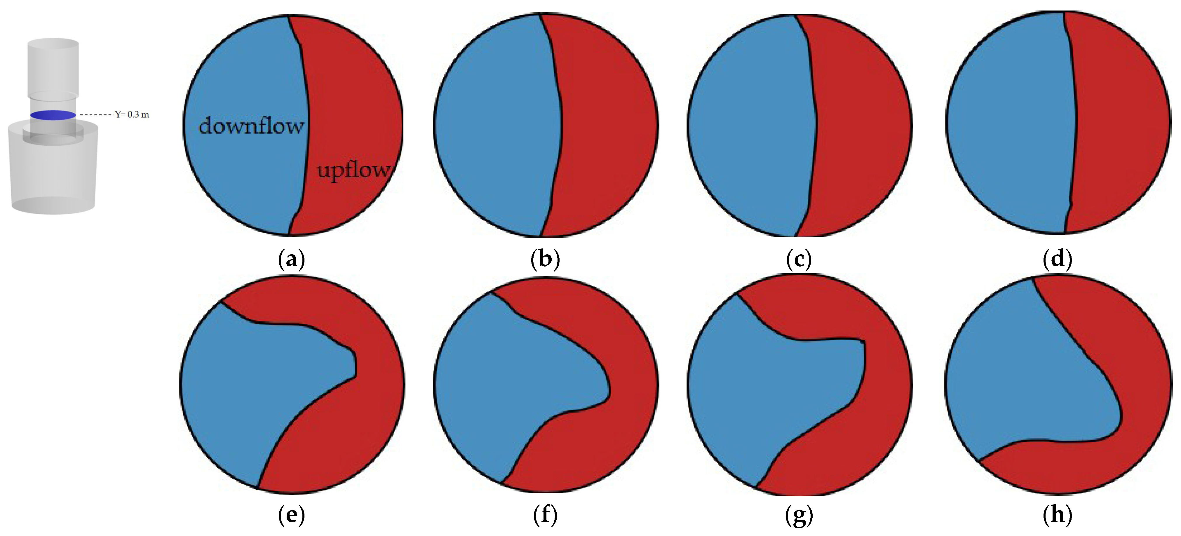
3.2. Flow Field
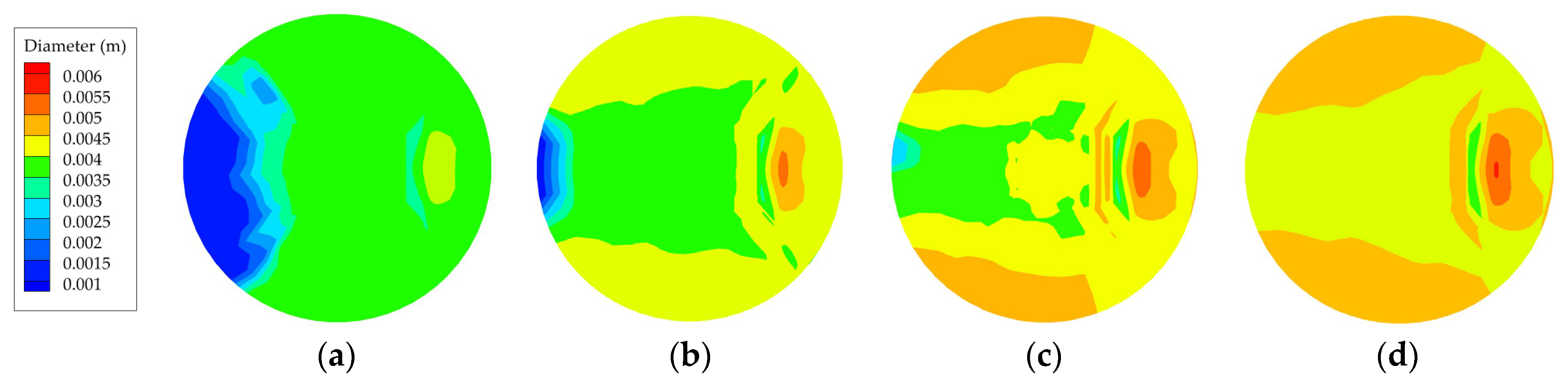
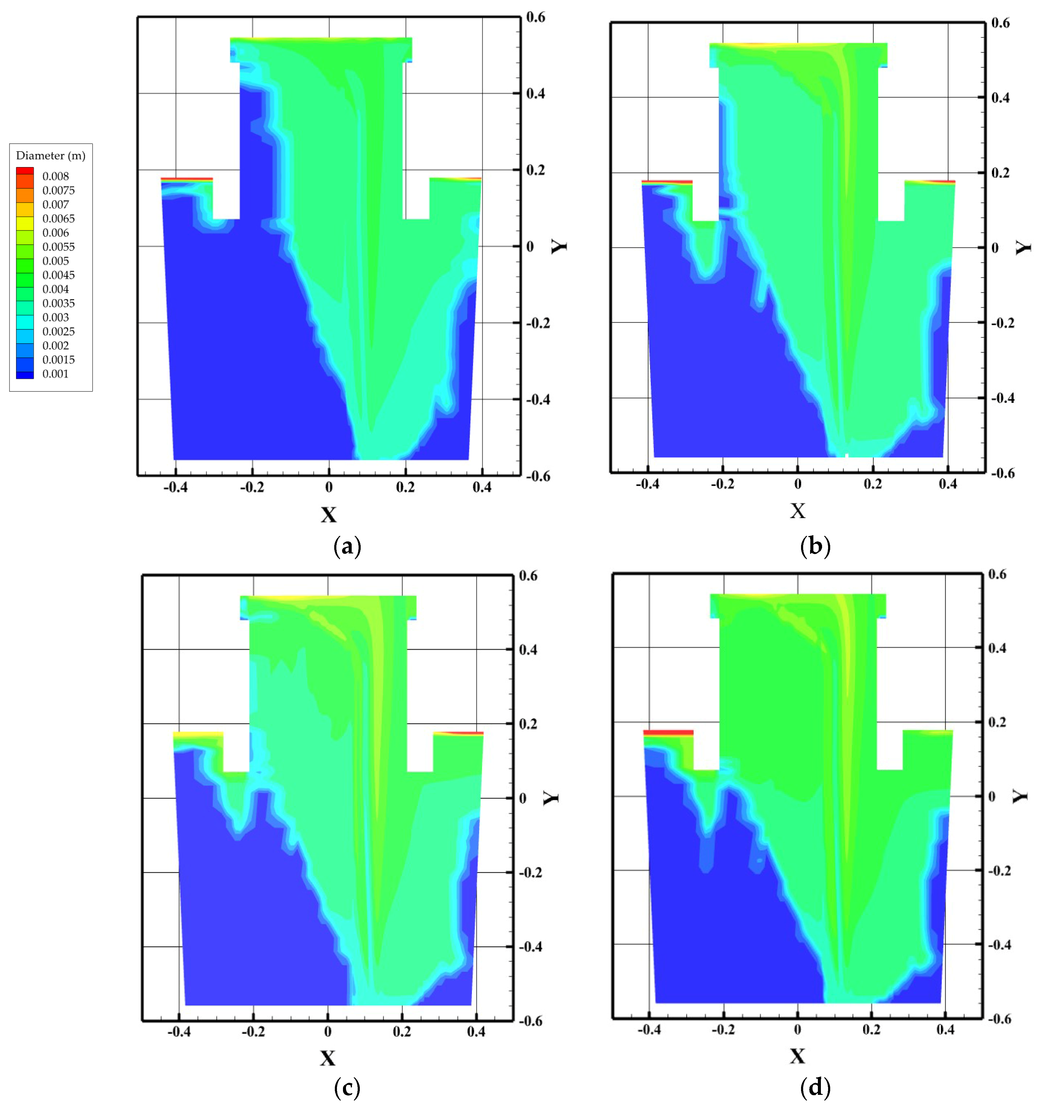
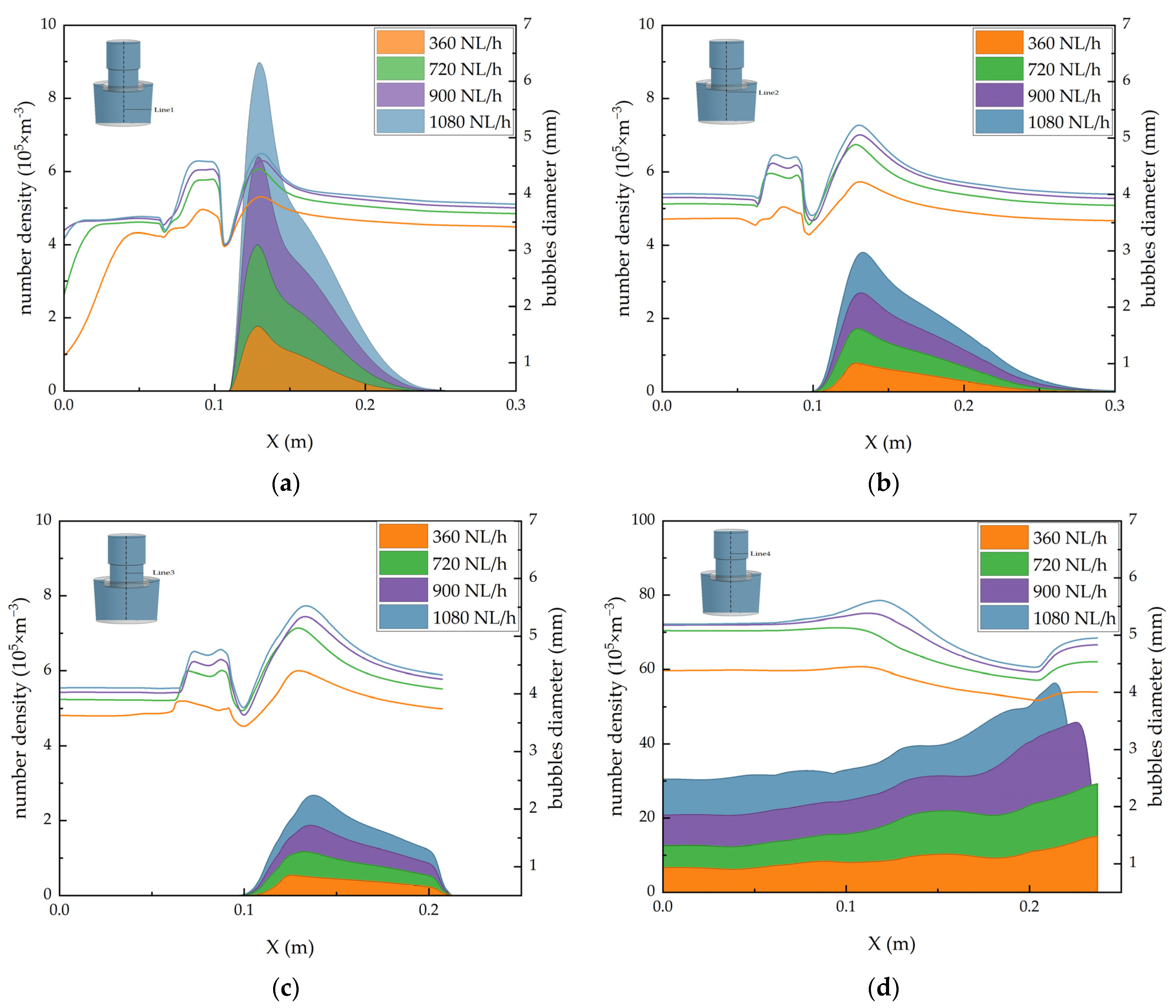
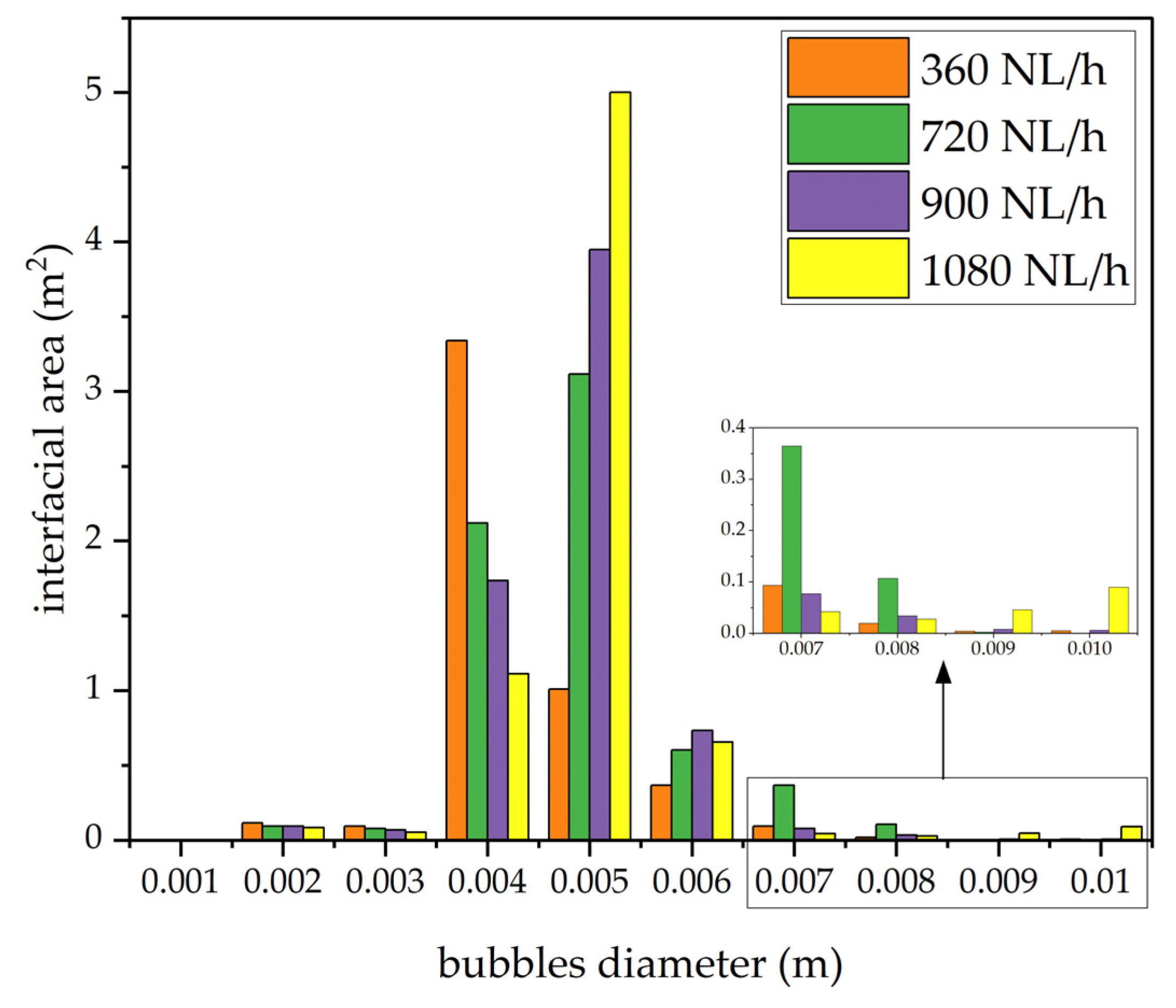
3.3. Local Bubble Size Distribution
4. Conclusions
Author Contributions
Funding
Data Availability Statement
Conflicts of Interest
References
- Statistical Bulletin on National Economic and Social Development of the People’s Republic of China for 2021. Available online: http://www.stats.gov.cn/tjsj/zxfb/202202/t20220227_1827960.html (accessed on 28 February 2022).
- Qi, F.S.; Liu, J.X.; Liu, Z.Q.; Cheung, S.; Li, B.K. Characterization of the Mixing Flow Structure of Molten Steel in a Single Snorkel Vacuum Refining Furnace. Metals 2019, 9, 400. [Google Scholar] [CrossRef] [Green Version]
- Chen, H.; Lei, H.; Jiang, J.M.; Geng, D.Q. Water modeling experiment on flow field of liquid steel during single snorkel RH vacuum refining process. J. Iron Steel Res. 2016, 28, 10–14. [Google Scholar]
- Dai, W.X.; Cheng, G.G.; Zhang, G.L.; Huo, Z.D. Investigation of Circulation Flow and Slag-Metal Behavior in an Industrial Single Snorkel Refining Furnace (SSRF): Application to Desulfurization. Metall. Mater. Trans. 2020, 51, 611–627. [Google Scholar] [CrossRef]
- Yang, X.M.; Zhang, M.; Wang, F.; Duan, J.P.; Zhang, J. Mathematical Simulation of Flow Field for Molten Steel in an 80-ton Single Snorkel Vacuum Refining Furnace. Steel Res. Int. 2012, 46, 55–82. [Google Scholar] [CrossRef]
- Qin, Z.; Pan, H.M.; Zhu, M.T.; Cheng, G.G.; Zhang, J. Modeling study on flow behaviors of molten steel in single snorkel refining furnace. Iron Steel Gangtie 2011, 46, 22–25. [Google Scholar]
- Zhang, Y.X.; Chen, C.; Lin, W.M.; Yu, Y.C.; E, D.Y.; Wang, S.B. Numerical Simulation of Tracers Transport Process in Water Model of a Vacuum Refining Unit: Single Snorkel Refining Furnace. Steel Res. Int. 2020, 91, 2000022. [Google Scholar] [CrossRef]
- Ouyang, X.; Lin, W.; Luo, Y.; Zhang, Y.; Fan, J.; Chen, C.; Cheng, G.G. Effect of Salt Tracer Dosages on the Mixing Process in the Water Model of a Single Snorkel Refining Furnace. Metals 2022, 12, 1948. [Google Scholar] [CrossRef]
- Duan, J.P.; Zhang, Y.L.; Yang, X.M.; Cheng, G.G.; Zhang, J.; Guo, H.J. Experiment research on decarburization technology of 80 t single snorkel vacuum refining equipment. Iron Steel Gangtie 2011, 46, 21–25. [Google Scholar]
- You, Z.M.; Cheng, G.G.; Wang, X.C.; Qin, Z.; Tian, J.; Zhang, J. Mathematical Model for Decarburization of Ultra-low Carbon Steel in Single Snorkel Refining Furnace. Metall. Mater. Trans. B Process Metall. Mater. Process. Sci. 2014, 46, 459–472. [Google Scholar] [CrossRef]
- Chen, G.J.; He, S.P. Circulation flow rate and decarburization in the RH degasser under low atmospheric pressure. Vacuum 2018, 153, 132–138. [Google Scholar] [CrossRef]
- Lei, H. Study on Deep Decarburization Technology of RH-MFB for IF Steel. Shandong Metall. 2020, 42, 44–48. [Google Scholar]
- Geng, D.Q.; Zhang, J.X.; Wang, K.; Wang, P.; Liang, R.Q.; Liu, H.T.; Lei, H. Simulation on Decarburization and Inclusion Removal Process in the Ruhrstahl–Heraeus (RH) Process with Ladle Bottom Blowing. Metall. Mater. Trans. B Process Metall. Mater. Process. Sci. 2015, 46, 1484–1493. [Google Scholar] [CrossRef]
- Rui, Q.X.; Cheng, G.G. A Desulphurization Mathmatical Model for Single Snorkel Refining Furnace. Adv. Mater. Res. 2012, 476–478, 340–345. [Google Scholar] [CrossRef]
- Duan, J.P.; Zhang, Y.L.; Yang, X.M.; Cheng, G.G.; Zhang, J. Desulfurization behavior of an 80 t multifunctional single snorkel vacuum refining furnace. Lian Gang 2011, 27, 44–48. [Google Scholar]
- Dou, W.; Lei, H.; Zhu, M. Numerical simulation for metallurgical transfer in 70 t single snorkel RH. J. Cent. South Univ. 2019, 50, 1284–1290. [Google Scholar]
- Chen, G.J.; Yang, J.; Li, L.; Zhang, M.; He, S.P. Thermodynamic and experimental study on CO2 injection in RH decarburization process of ultra-low carbon steel. J. CO2 Util. 2021, 50, 101586. [Google Scholar] [CrossRef]
- Chen, S.F.; Lei, H.; Li, Q.; Ding, C.Y.; Dou, W.X.; Chang, L.S. Effect of Nonequilibrium Decarburization on Inclusion Transfer During Single Snorkel RH Vacuum Refining. JOM 2022, 74, 1578–1587. [Google Scholar] [CrossRef]
- Chen, S.F.; Lei, H.; Wang, M.; Yang, B.; Dou, W.X.; Chang, L.S.; Zhang, H.W. Ar-CO-liquid steel flow with decarburization chemical reaction in single snorkel refining furnace. Int. J. Heat Mass Transf. 2020, 146, 118857. [Google Scholar] [CrossRef]
- Uemura, K.; Takahashi, M.; Koyama, S. Production of ultra-low carbon steel by RH degasser. Kobe Res. Dev. Jpn 1991, 41, 24–27. [Google Scholar]
- Takahashi, M.; Matsumoto, H.; Saito, T. Mechanism of decarburization in RH degasser. ISIJ Int. 1995, 35, 1452–1463. [Google Scholar] [CrossRef] [Green Version]
- Zhao, L.H.; Guo, J.L.; Xu, J.L.; Zhang, C.J. Complex bubble formation in the vacuum chamber and the up leg of the Rheinsahl-Heraeus. Chin. J. Eng. 2018, 40, 453–460. [Google Scholar]
- Hernandez, L.; Julia, J.E.; Chiva, S.; Paranjape, S.; Ishii, M. Fast classification of two-phase flow regimes based on conductivity signals and artificial neural networks. Meas. Sci. Technol. 2006, 17, 1511–1521. [Google Scholar] [CrossRef]
- Wu, Y.D.; Liu, Z.Q.; Wang, F.; Li, B.K.; Gan, Y. Experimental investigation of trajectories, velocities and size distributions of bubbles in a continuous-casting mold. Powder Technol. 2021, 387, 325–335. [Google Scholar] [CrossRef]
- Dai, W.X.; Cheng, G.G.; Li, S.J.; Huang, Y.; Zhang, G.L. Numerical Simulation of Multiphase Flow and Mixing Behavior in an Industrial Single Snorkel Refining Furnace: Effect of Bubble Expansion and Snorkel Immersion Depth. ISIJ Int. 2019, 59, 2228–2238. [Google Scholar] [CrossRef] [Green Version]
- Dai, W.X.; Cheng, G.G.; Li, S.J.; Huang, Y.; Zhang, G.L.; Qiu, Y.L.; Zhu, W.F. Numerical Simulation of Multiphase Flow and Mixing Behavior in an Industrial Single Snorkel Refining Furnace (SSRF): The Effect of Gas Injection Position and Snorkel Diameter. ISIJ Int. 2019, 59, 1214–1223. [Google Scholar] [CrossRef] [Green Version]
- Chen, G.J.; He, S.P. Numerical simulation of Argon-Molten steel two-phase flow in an industrial single snorkel refining furnace with bubble expansion, coalescence, and breakup. J. Mater. Res. Technol. 2020, 9, 3318–3329. [Google Scholar] [CrossRef]
- Luo, H.; Svendsen, H.F. Theoretical model for drop and bubble breakup in turbulent dispersions. AIChE 1996, 42, 1225–1233. [Google Scholar] [CrossRef]
- Prince, M.J.; Blanch, H.W. Bubble coalescence and break-up in air-sparged bubble columns. AIChE 1990, 36, 1485–1499. [Google Scholar] [CrossRef]
- Ansys. ANSYS-FLUENT Version 22.R1 User Guide; ANSYS Inc.: Canonsburg, PA, USA, 2022. [Google Scholar]
- Liao, Y.X.; Lucas, D. A literature review of theoretical models for drop and bubble breakup in turbulent dispersions. Chem. Eng. Sci. 2009, 64, 3389–3406. [Google Scholar] [CrossRef]


Disclaimer/Publisher’s Note: The statements, opinions and data contained in all publications are solely those of the individual author(s) and contributor(s) and not of MDPI and/or the editor(s). MDPI and/or the editor(s) disclaim responsibility for any injury to people or property resulting from any ideas, methods, instructions or products referred to in the content. |
© 2023 by the authors. Licensee MDPI, Basel, Switzerland. This article is an open access article distributed under the terms and conditions of the Creative Commons Attribution (CC BY) license (https://creativecommons.org/licenses/by/4.0/).
Share and Cite
Qi, F.; Ye, N.; Liu, Z.; Cheung, S.C.P.; Li, B. Numerical Simulation of Bubble Size Distribution in Single Snorkel Furnace (SSF) with Population Balance Model (PBM). Metals 2023, 13, 212. https://doi.org/10.3390/met13020212
Qi F, Ye N, Liu Z, Cheung SCP, Li B. Numerical Simulation of Bubble Size Distribution in Single Snorkel Furnace (SSF) with Population Balance Model (PBM). Metals. 2023; 13(2):212. https://doi.org/10.3390/met13020212
Chicago/Turabian StyleQi, Fengsheng, Nan Ye, Zhongqiu Liu, Sherman C. P. Cheung, and Baokuan Li. 2023. "Numerical Simulation of Bubble Size Distribution in Single Snorkel Furnace (SSF) with Population Balance Model (PBM)" Metals 13, no. 2: 212. https://doi.org/10.3390/met13020212