Research on the Curvature Prediction Method of Profile Roll Bending Based on Machine Learning

Abstract

Roll-bending technology has a high degree of flexibility and does not require special molds. However, based on the existing plastic mechanics theory and finite element simulation, it is difficult to accurately analyze the complex spatial relationship of profile roll forming. Therefore, a fixed-curvature prediction model is constructed based on XGBoost (extreme gradient boosting), and the coupling effect of the process parameters and material performance parameters on the roll-forming process is explored. Combined with a Bayesian optimization algorithm, the hyperparameters of the fixed-curvature prediction model are optimized. In addition, based on the prediction result of the fixed curvature, a variable-curvature prediction model is established using the conditional random field (CRF). To further improve the prediction accuracy, an error compensation network is added after the result of the CRF in order to map the discrete sequence to the continuous sequence. The experimental results show that the mean square error (MSE), mean absolute error (MAE), and mean absolute percentage error (MAPE) predicted by the models above are much smaller than other methods, which verifies the superiority of the prediction models.

1. Introduction

There is a vast aerospace market for high-precision bending parts [1], such as rocket booster frame rings, aircraft wind-driven structural fuselage, etc. Roll-bending technology does not require exclusive molds, is not limited by the length of the profile, and has broad applicability. It can well support the production needs of high-precision bending parts in the aerospace field. However, the complex force and deformation in the roll-forming process lead to uncontrollable springback, which has a great impact on the dimensional accuracy of the product.

Many scholars have devoted themselves to the study of bending springback. In the field of mathematical modeling, Desinghege et al. [2] studied the degenerative behavior of magnesium alloys from a microscopic perspective based on mathematical theory. Based on the experimental results, an analytic equation was established to explain the effect of grain size on magnesium springback. Su et al. [3] proposed the five-boundary conditional distribution function of the forming angle. The stress, strain, and springback of the sheet during roll forming under three different angle distribution functions were studied. The results showed that the stress, strain, and springback of each pass based on the increment of the forming angle under the condition of five boundaries in the roll-forming process were smaller than those of other forming angle distribution methods. To obtain a higher forming accuracy of spatially variable-curvature bending metal tubes, Wang et al. [4] proposed a numerical approximate springback prediction and compensation method considering SVC MT section distortion. The experimental results showed that the position deviation of each node was less than 1.4% and the average position deviation was less than 0.80% after springback compensation. In the field of finite element modeling, Fan et al. [5] studied the springback characteristics of TRBs by the finite element code Abaqus/USDFLD and the cylindrical bending test, providing an important opportunity to further understand TRB springback characteristics. Chang et al. [6] studied the bending springback of medium manganese steel under different conditions through experiments and simulations. Material models with a constant and variable modulus of elasticity were established. The V-shaped bending test at a constant and variable modulus of elasticity was simulated and compared with the experimental results. The simulation results of the variable modulus of elasticity were closer to the experimental results, which proves the importance of considering the change in elastic modulus of unloading in the numerical simulation of manganese steel. Sharma et al. [7] established a springback prediction analysis model combining the effects of anisotropy and strain hardening, and simulated the springback behavior of double-layer metal plates by using the Hill anisotropic yield criterion in Abaqus software. Liu et al. [8] discussed the resilience energy of UHSS in cold forming through simulation and experimental methods. At the same time, a three-dimensional finite element model was established by using COPPA RF and MSC MARC to analyze the CRF process. Julsri et al. [9] performed experimental bending tests and their corresponding finite element simulations. The springback effect of AHS steel grade 980 during V-bending was studied.

However, in recent years, traditional mechanical analysis methods have been difficult to further develop in the field of bending springback, and it has been difficult to make breakthroughs [10]. Mechanical analysis methods can only be analyzed in a positive direction. However, the development of artificial intelligence has brought a new way of thinking, which avoids that limitation, and reverses the forming law through actual data. Through the analysis of actual data by such methods, the change law of springback in bending forming is learned, so as to accurately predict the final result of deformation.

For shaft tube parts, Choi et al. [11] studied the continuous bending forming of hairpins in drive motors, extracted training data from finite elements, and used artificial intelligence algorithms to compensate for the springback of the forming process. Sun et al. [12] constructed an optimization framework containing a GRU-based deep-learning network as a prediction module, and proposed the Pb-NSGA-III algorithm to achieve the accurate prediction of the bending and springback of tube shaft parts. Lu et al. [13] established a machine-learning model based on finite element simulation data and optimized forming paths for the stretch-and-bend process. For sheet metal parts, Cruz et al. [14] used a shallow artificial neural network to identify constitutive model parameters by using the force–displacement curve obtained by the bending experiment. Based on the learning ability of shallow artificial neural networks, the bending springback was predicted by the dataset extracted from finite elements. Liu et al. [15] used a deep neural network training method based on theoretical guidance to predict sheet metal bending springback. Compared with conventional springback compensation methods, the development cycle was shortened, and the cost and calculation requirements were reduced. Xu et al. [16] and Li et al. [17] proposed to use the genetic algorithm (GA) and sparrow search algorithm (SSA) to predict the cold bending springback of the hull based on the backpropagation neural network (BPNN), which greatly improved the prediction accuracy and prediction speed. Wasif et al. [18] analyzed the influence of various parameters on the bending springback of JSH590 steel by the V-shaped bending test, and applied the genetic algorithm to optimize the process parameters of minimum springback. Serban et al. [19] developed an artificial neural network model with sheet thickness, punch radius and friction coefficient as the input parameters to predict the bending springback of cylindrical plates. Trzepiecinski et al. [20] further considered anisotropy, taking an anisotropic cold-rolled steel plate as the research object, and used an artificial neural network based on multilayer perceptron combined with the genetic algorithm to predict bending springback. In addition to the conventional bending process, Liang et al. [21] proposed a chain die design method using a multi-section compensation strategy in the field of chain die forming, and used the nondominated ranking genetic algorithm II to minimize the deviation of the calculated cross-sectional springback profile from the required geometry. The results showed that the springback and longitudinal arch were reduced by using the proposed mold design method. El et al. [22] took the deep drawing process as the research object, and proposed an optimization method combining finite element, experimental, artificial neural network and particle swarm optimization to optimize the quality of stamped parts, especially to solve the springback problem. In order to optimize the stamping forming quality of high-strength steel, Jia et al. [23] used the B-Benhnken test to construct a multi-objective optimization function of the response surface between the maximum springback displacement and the maximum thinning ratio process parameters. The objective function was solved by using the NSGA-II algorithm to obtain the optimal solution. Akrichi et al. [24] introduced the neural network method into the quality prediction of the single-point incremental forming process, so as to formulate the optimal toolpath, incremental step size, spindle speed and other parameters. Ciubotariu et al. [25] introduced artificial intelligence methods into the welding springback problem, and applied genetic algorithms to optimize weld line positioning, combining multiple software platforms to evaluate the data and perform experimental verification. In addition to the springback that appears immediately after processing, Kong et al. [26] also took time-dependent springback as the research object and proposed a straightness dynamic evaluation method considering time-dependent springback in the bending–straightening process with the GA-BP neural network as the main part, and established a rapid prediction model of time-dependent springback.

Artificial intelligence research studies the inherent laws of complex forming relationships in roll bending through the intelligent analysis model and machine-learning method. The current artificial intelligence methods and forming mechanisms have not achieved deep integration. There are certain limitations in the precise characterization and analysis of the coupling effect of complex factors. The theoretical research foundation is relatively weak, and the spatial parameter correlation constraints and conditional criteria are insufficient. The analysis system of profile roll bending under complex influence conditions has not been scientifically established, which affects the effectiveness of the analysis. Therefore, the artificial intelligence research of complex forming of profile rolling is still in the exploratory stage.

Given the background that the basic theory and standard technology of roll-bending springback deformation of profiles are difficult to further develop, the influence of springback deformation of profile roll bending is analyzed, and the characterization and measurement methods of the roll-bending feature space are studied. Using the idea of a deep integration of mechanism research and artificial intelligence, a theoretical model for the intelligent analysis of roll-bending forming is established. A smart analysis method for springback deformation of roll-bending forming is designed to reveal the complex forming laws of the profile rolling.

2. Prediction Model for Springback of Fixed Curvature Based on XGBoost

2.1. Analysis of Influencing Factors of Springback and Data Preprocessing

The springback is the main factor affecting the forming accuracy of the roll bending, and the main influencing factors of springback are the material properties, geometric parameters, and forming process parameters of the profile. Under the condition that the material and shape of the profile remain unchanged, the external factors that affect the springback of roll forming (the process parameters) are studied. The process parameters selected are roll spacing, feed rate, reduction, and the radius of curvature before springback. Part of the data is shown in

Table 1. Part of the dataset.

Roll Spacing (mm)	Feed Rate (mm/s)	Reduction (mm)	Radius of Curvature before Springback (mm)
465	14.65	3	166,111
		6	24,901
		9	8098
		12	4426
		15	3207
		18	2385
		21	1837
		24	1591

.

Construction of Density Clustering Features

The springback amount of the profile is $R_s$ (the mechanical bending radius of the profile before springback) minus $R_e$ (the measured bending radius of the profile after springback). $R_s$ is shown in Equation (1). In Equation (1), $R_r$ is the radius of the lower roller, m is the reduction amount, h is the thickness of the profile, and $L_0$ is the distance from the lower roller to the upper roller.

$$R_s= -\frac{2R_{r}m+2hm+L_0^2+m^2}{2m}$$

(1)

The springback amount $\Delta$R is shown in Equation (2).

$$∆R=R_{s }- R_e$$

(2)

It can be seen from Equation (1) that when the roller parameters of the roll brake are unchanged, $R_s$ is only related to m and $L_0$. Therefore, $R_s$ and $L_0$ are repeated features, and the $L_0$ is removed from the parameter features to reduce the learning pressure of the model.

The elastoplastic performance of the profile affects the degree of springback, so this factor must be taken into account to improve the effect of model learning. The clustering method is used to divide the data into k different categories, arrange them based on the degree of springback, and assign them as 1 to k. The more significant the value, the greater the degree of springback, providing a valuable reference for the training of the model feature. The new features are constructed using the clustering algorithm proposed by Ji and Lei [27], which is called density clustering.

Suppose there is a dataset $S=\left\{X_i\right\}$. For any data point $X_i$ in $S$, the local density ${\rho }_i$ and the distance ${\sigma }_i$ can be defined. ${\rho }_i$ is the sum of the number of data points in the dataset whose distance from the $i$ point is less than a specific value. ${\sigma }_i$ describes how close point $i$ is to other points whose local density is more significant than point $i$. It can be concluded that for a point $i$, if its local density ${\rho }_i$ is larger than other points, and the distance ${\sigma }_i$ from other points with higher local density is also larger, then point $i$ is a possible center point of a class. To select the cluster center, the quantity $\gamma$ is introduced, and the definition of $\gamma$ is shown in Equation (3).

$${\gamma }_i={\rho }_i{\sigma }_i$$

(3)

The size of the value $\gamma$ can be a criterion for measuring whether it is possible to become a cluster center, so it is necessary to screen based on the $\gamma$ value of the data points, and find the points with the largest $\gamma$, which are the cluster centers.

For data with known features, the first step in clustering is to have a clear definition of similarity, and only with similarity can the relationship between samples be accurately defined. Then, with the process parameter $x$ and the profile parameter $y$, sample data can be obtained as $D_i=(x_i,y_i,∆R_i)$, assuming that $D_1=(x_1,y_1,∆R_1)$ and $D_2=(x_1,y_1,∆R_1)$ are two different samples in the data set. Its similarity is defined as Equation (4).

$$\mathrm{dist}=\alpha d(x_1,x_2)+\beta d(y_1,y_2)+\gamma d(∆R_1,∆R_2)$$

(4)

In Equation (4), $d(x,y)$ represents the Euclidean distance between $x$ and $y$, and $\alpha$, $\beta$, and $\gamma$ are weight coefficients. The distribution of data points in the coordinate system after clustering is shown in Figure 1. The horizontal axis represents the reduction amount m, and the vertical axis represents the $∆R$.

Based on the definition of similarity, the samples are clustered. The springback of profiles can be roughly divided into three regions: elastic region, plastic dominant region, and elastoplastic region. Therefore, in Figure 1, the data points are divided into three clusters.

Profiles show different springback in different regions. Usually, the springback is larger in small-curvature forming, more minor in large-curvature forming, and the springback in the middle area is more complicated. Clustering is used to find three cluster centers in order to divide the data into three clusters, and each cluster corresponds to a different degree of springback of the profile. The construction of new features is completed based on clustering, and part of the data is shown in

Table 2. Dataset after adding new features.

Roller Spacing (mm)	Feed Rate (mm/s)	Reduction (mm)	Degree of Springback	Radius of Curvature (mm)
465	14.65	3	3	166,111
		6	3	24,901
		9	2	8098
		12	2	4426
		15	2	3207
		18	1	2385
		21	1	1837
		24	1	1591

.

2.2. Comparison and Analysis of Machine-Learning Methods

In fixed-curvature roll bending, the final output result is the average bending radius of the entire profile measured. The factors that affect the bending radius include the reduction, distance between lower rollers, and properties of the profile itself. That is, the independent variable is a multi-dimensional feature vector, and the dependent variable is the curvature radius. Regression algorithms in machine learning fit this process. Support vector machine regression (SVR), ridge regression, linear regression, decision tree regression, and XGBoost [28] are all regression algorithm models widely used for various problems in current machine learning. By comparison, XGBoost has higher accuracy, and it can also perform a second-order Taylor expansion on the loss function to facilitate the application of a suitable loss function. XGBoost also adds a regular term to the objective function, which can effectively control the complexity of the model, control the size of the model parameters, and effectively solve the problem of model overfitting. For the problem of small samples, the learned model has better generalization and cannot easily fall into optimal local results. The XGBoost algorithm is selected.

2.3. Construction of Springback Prediction Model with Fixed Curvature Based on XGBoost

Based on the above analysis of the advantages of XGBoost, an intelligent coupling influence analysis model of fixed curvature based on XGBoost is proposed. Based on the complex nonlinear mechanical properties of the elastic, plastic and elastoplastic state distribution of materials, the coupling influence analysis studies the basic law of springback deformation under the coupling of material parameters and forming mechanical parameters.

Therefore, the coupled effects analysis is a classification regression problem based on the elastoplastic forming relationship. The objective function of multi-factor coupling affects is established: $R_e=SC(M_p,M_G,F)$; $R_e$ is the radius of curvature after forming, $M_p$ is the performance parameter of the material, $M_G$ is the geometric parameter of the material, $F$ is the forming process parameter, and SC is the forming relationship function under the coupling action. Based on XGBoost, with the regression tree as the base model, the coupling analyzer (SC) of complex effects is constructed by using the gradient boosting method through the associated regression tree joint decision. Additionally, Bayesian optimization is used to adjust the hyperparameters of the model to optimize the performance ability of the model. As shown in Figure 2.

In the process of fixed-curvature roll bending, each data record corresponds to one experiment (one profile). The reduction amount, the feed rate, the curvature radius before springback, and the new features constructed above are selected to form the characteristics of the data set. Since the chosen model belongs to the tree model, the data features of different orders of magnitude do not affect the model results, so there is no need to normalize the features. Assuming that the data sample size is $n$, the final data format is shown in Equation (5). $P$ represents the reduction amount, $V$ represents the feed rate, $E$ represents the constructed new feature, $R_s$ represents the radius of curvature before springback, and $R_e$ represents the radius of curvature measured after springback.

$$\left[\begin{array}{ccccc}{P}_1& V_1& E_1& R_{s_1}& R_{e_1}\\ P_2& V_2& E_2& R_{s_2}& R_{e_2}\\ \dots & \dots & \dots & \dots & \dots \\ P_n& V_n& E_n& R_{s_n}& R_{e_n}\end{array}\right]$$

(5)

The primary process of the springback prediction model with fixed curvature based on XGBoost includes current tree node splitting, tree structure scoring, updating the strong classifier model, and Bayesian optimization hyperparameters. The key to the algorithm is how to divide the current node. The gain after a split is shown in Equation (6):

$$\mathrm{Gain}=\frac{1}{2}\left(\frac{G_L^2}{H_L+\lambda }+\frac{G_R^2}{H_R+\lambda }- \frac{{{(G}_L+G_R)}^2}{H_L+H_R+\lambda }\right)- \gamma$$

(6)

where $G_L$ and $G_R$, respectively, represent the accumulated sum of the first-order partial derivatives of the left and right subtrees containing the samples, $H_L$ and $H_R$, respectively, represent the accumulated sum of the second-order partial derivatives of the left and right subtrees containing the samples, $\lambda$ represents the control parameters before the regular term, $\gamma$ represents the complexity of the tree structure, and the more leaf nodes, the greater the value of $\gamma$. Calculate $P, V, E,{ R}_s$ and $R_e$ when splitting, select the splitting feature with the highest gain and its splitting position, and perform the splitting operation on this node to split two new left and right leaf nodes. The above steps are performed recursively until the score of this tree meets the requirements, at which time the weak learner training of the current round is completed. Finally, the strong learner is updated using the current weak learner.

To make the XGBoost model perform better, in addition to the parameter learning during the training process, the adjustment of hyperparameters is also essential. The hyperparameters that XGBoost can adjust include the depth of the tree, the maximum number of leaf nodes, the learning rate, and the regularity. Bayesian optimization is used to adjust the hyperparameters. The algorithm will eventually generate multiple strong classifiers with different hyperparameters in the Bayesian optimization, and a better prediction model can be obtained by screening them.

2.4. Realization of Springback Prediction Model with Fixed Curvature Based on XGBoost

First, the roll-bending experiment is performed to obtain the data set shown in Equation (5). Separate 70% of the dataset as the training set and the other 30% as the test set. Build the XGBoost springback prediction training model and input the training set into the model for training. The model structure of XGBoost plus Bayesian optimization is shown in Figure 3.

The final evaluation index of the model is the mean square error of the radius of curvature after springback. Since it is training with small sample data, to prevent overfitting, an $L_2$ regular term is added, and the weight can be adjusted as a hyperparameter. In addition, limiting the height of the tree to a relatively low range can also prevent overfitting to a certain extent. After model training is complete, the test set is used to evaluate the current model and record the results. Different models are obtained by adjusting hyperparameters through Bayesian optimization, and the hyperparameters are optimized based on the results until the set upper limit of the number of times is reached.

The algorithm steps are shown in Algorithm 1:

Algorithm 1: Fixed-curvature springback prediction algorithm based on XGBoost

Input: training set dataset_train and test set dataset_test

Output: Springback prediction model f

Step 1: Initialize the parametric model $\widehat{f}$.

Step 2: Iteratively generate M weak learners and update the strong learner $\widehat{f}$ as follows:

(1) Find the splitting location with the greatest gain from the current node splitting  (2) Split to get new left and right leaf nodes  (3) Repeat the above two steps until the current tree structure score meets the re-quirements or reaches the upper limit of splitting  (4) Update the strong learner $\widehat{f}$, jump out if the number of weak learners reaches M; otherwise, find the residual of the current weak learner, and go to step 1)

Step 3: If the prediction result of the model $\widehat{f}$ reaches the set standard or the update times reaches the set upper limit, go to Step 4; otherwise, go to Step 2.

Step 4: Use the test set to evaluate the model and store the current hyperparameter combination and model evaluation score.

Step 5: If the set upper limit of Bayesian optimization times is reached or the result meets the expected standard, go to Step 6; otherwise, go to Step 1.

Step 6: Select the optimal hyperparameter combination from the searched hyperparameter combinations.

Step 7: Use the optimal hyperparameter combination selected in Step 6 to construct a prediction model f, f(P,V,E,RS) = RE.

Algorithmic step 1 randomly initialized a set of model hyperparameters, including the maximum depth of the tree, learning rate, and regularization weights. Steps 2 to 4 are the learning process of the current hyperparameter combination model, evaluate the current model, and store the evaluation result and the hyperparameter combination. Steps 5 to 7 are the Bayesian optimization process, exploring the optimal hyperparameter combination, and using the optimal hyperparameter combination to build the final prediction model.

3. Variable-Curvature Springback Prediction Model Based on Conditional Random Field

3.1. Comparison and Analysis of Machine-Learning Methods

In the process of roll bending, there are big differences between variable-curvature forming and fixed-curvature forming process. The factors affecting the forming process in variable-curvature forming are not only the parameters of the material itself at each stage and the process parameters in the forming process, but also affected by the previous stage and the next stage of forming, and the various influencing factors are also changing irregularly. Therefore, using fixed-curvature prediction model to predict variable-curvature roll springback produces a large error, as shown in Figure 4. $S_i$ represents the state of the i-th position of the profile, including the shape parameters, performance parameters, and process parameters of the material at the current position.

By using the fixed-curvature prediction model, the springback value can be known when the influences before and after a certain stage of the profile are the same, and the actual value of the profile springback can be obtained by experimental measurement. Then for a variable-curvature profile, an inaccurate variable-curvature radius sequence can be predicted by the fixed-curvature model, and an accurate variable-curvature radius sequence can be obtained by actual measurement. The task of variable-curvature forming prediction is to predict this exact sequence base on this inaccurate sequence. That is, a sequence-to-sequence prediction problem.

Neural networks are widely used in dealing with sequence-to-sequence problems, including recurrent neural network [29] and its variant long-short-term memory network [30], bidirectional long-short-term memory neural network, GRU (Gate Recurrent Unit), and conditional random field (CRF) [31] and so on. By comparison, in the task of variable-curvature springback prediction, the output and output are both sequences, and the sequence is a chain structure, which has a specific correlation before and after, which meets the modeling requirements of CRF. The training of the undirected graph model does not depend on a large amount of data, and small-scale data can also obtain better results, which meets the requirements to the problems. Therefore, the CRF is used to establish a springback model of variable-curvature forming.

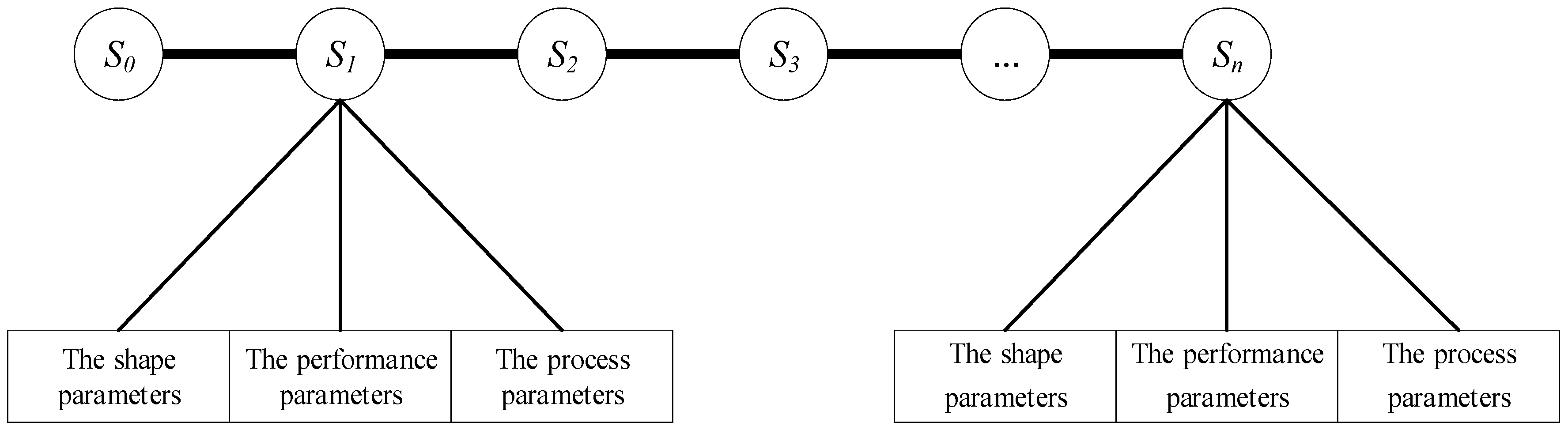
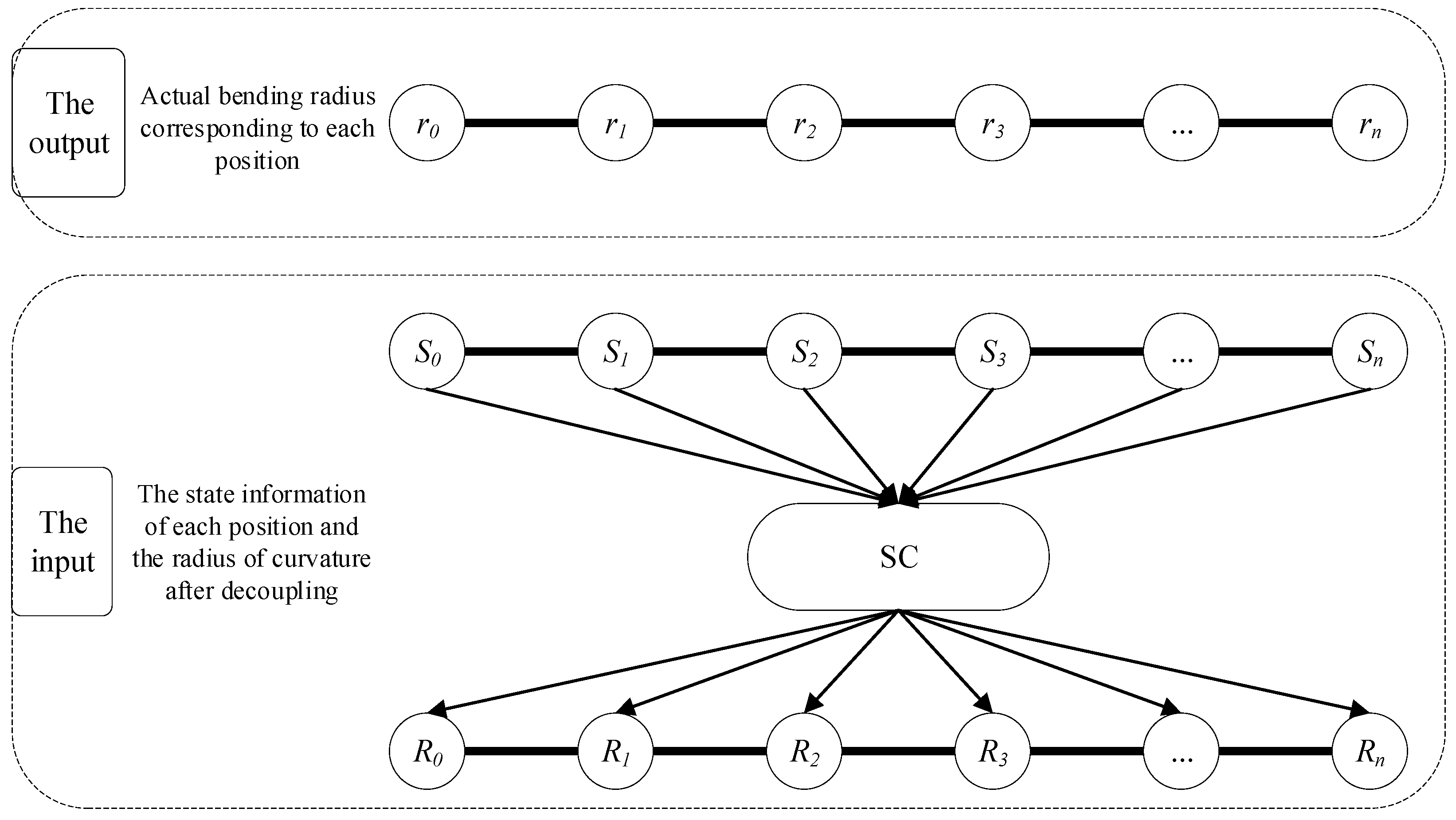
3.2. Construction of Variable-Curvature Springback Prediction Model Based on Conditional Random Field

The task of the variable-curvature springback prediction model is to correct the error of the sequence predicted by the fixed-curvature springback model to obtain the actual curvature radius sequence of the profile.

A variable-curvature springback prediction model based on conditional random fields is proposed. The model is based on the prediction of the fixed-curvature model. The input is the prediction result of the fixed-curvature model to the variable-curvature experiment, and the output is the actual measurement value of the variable-curvature experiment. Since the conditional random field prediction is a sequence of a series of discrete values, to further reduce the error, an error network needs to be added to map discrete values to continuous values, making the sequence of prediction results smoother and more accurate. A fully connected neural network is used to correct the error.

The structure of the springback prediction model based on the conditional random field variable curvature is shown in Figure 5.

In the process of variable-curvature roll bending, the data corresponding to each profile is a sequence, which is composed of the process parameters corresponding to each position of the profile, including the reduction amount, the speed of reduction, the feed rate, and the average radius of curvature after springback. For each position of the profile, the input required by the fixed-curvature model is included, so the curvature radius $R_p$ can be predicted for each position of the profile using the fixed-curvature model, which means the radius of curvature of the profile when the front and back stages have the same effect on the current position. The actual measured radius of curvature is $R_f$. The conditional random field is a classification model, so the original output needs to be discretized. Using each centimeter of profile length as a data point of the sequence, the sum of the raw point data in this interval is summed and averaged as the value of the current data point. Assuming that the length of a data sequence after discretization is $n$, the format of the final data is shown in Equation (7):

$$\left[\begin{array}{cccc}{P}_1& V_1& R_{p_1}& R_{f_1}\\ P_2& V_2& R_{p_2}& R_{f_2}\\ \dots & \dots & \dots & \dots \\ P_n& V_n& R_{p_n}& R_{f_n}\end{array}\right]$$

(7)

where $P_i$ represents the reduction amount corresponding to position $i$, and $V_i$ represents the speed of reduction corresponding to position $i$. $R_p$ sequence is the observation sequence, and $R_f$ is the actual springback radius value sequence. The algorithm predicts the most probable output sequence $R_f$ by observing the correlation between the $R_p$ values and taking the reduction amount $P$ and the reduction speed $V$ as a reference. Assuming that the data sample is m, the final data format is shown in Equation (8):

$$\left[\begin{array}{cccc}{s}_{11}& s_{12}& \dots & s_{1n}\\ s_{21}& s_{22}& \dots & s_{2n}\\ \dots & \dots & \dots & \dots \\ s_{m1}& s_{m2}& \dots & s_{mn}\end{array}\right]$$

(8)

where $s_{ij}$ represents the state information of the $j$-th position in the i-th data. For example, $s_{11 }=\{P_1,V_1,R_{p1},R_{f1}\}$ includes the relevant information of the first position of the data sequence corresponding to the first profile.

The main processes of the variable-curvature springback prediction model based on CRF include calculating the empirical distribution of data, training model parameters by the quasi-Newton method, finding the optimal path, and discrete to continuous error compensation.

After the data set is constructed, the critical step of the algorithm is the training process. The learning methods of CRF include maximum likelihood estimation and regularized maximum likelihood estimation. The specific implementation algorithms include gradient descent and the quasi-Newton method (L-BFGS). The L-BFGS algorithm is used to train the conditional random field model in the study.

First, the empirical probability distribution $\tilde{P}(X,Y)$ is obtained using the known training data set, and the model parameters can be obtained by maximizing the log-likelihood function of the training data.

After the training of the CRF model is completed, the given input sequence is predicted to obtain the maximum possible label sequence, that is, the prediction process of the CRF. The prediction algorithm of the conditional random field is to find the output $Y$ that maximizes $P\left(Y\right|X)$ for a given $X$ and parameter $W$, which is a solution process of the optimal path of an undirected graph. To find the optimal solution, the most commonly used method is dynamic programming. The more typical Viterbi algorithm is used in the study.

3.3. Realization of Springback Prediction Model with Variable-Curvature Based on Conditional Random Field

The curvature radius sequence of each profile is obtained by using the fixed-curvature model, and this sequence will be used as the input of the CRF. The original data is discretized in segments, and a discrete sequence is obtained. The content of the feature sequence includes the reduction amount, speed of reduction, etc., and the actually measured curvature radius sequence is used as a label. Divide 70% of the dataset as the training set and the other 30% as the test set to construct a CRF model.

The length of the profile used in the variable-curvature experiment is 3 m, and the actual measured length is 2.6 m in the middle. From the position of 0.4 m in the data, set every 0.01 m as a stage, calculate the average value of the data between 0.01 m, and round it as characteristics of the current location. The discretized profiles are shown in Figure 6.

Before using the CRF model to predict the sequence, use the fixed-curvature model trained in Section 2 to predict the curvature radius sequence of the profile using the process parameters and profile parameters contained in each forming section. Figure 7 shows the input and output structure of the radius prediction model after variable-curvature springback based on CRF.

The SC is the fixed-curvature prediction model trained in Chapter 2, and the output result becomes the reference feature of the variable-curvature model, the data of different forming sections are input into the model as a whole, and the transition probability between each node in the undirected graph is obtained by the quasi-Newton method. After obtaining the conditional random field probability undirected graph model, the output sequence most likely corresponding to the input sequence is finally calculated by Viterbi. To make the predicted curvature radius curve smoother and more accurate, an error compensation network is added after the output sequence. The error compensation network uses a fully connected neural network to map discrete values to continuous values.

The algorithm steps are shown in Algorithm 2.

Algorithm 2: Curvature prediction after springback for variable-curvature roll bending based on conditional random fields

Input: training set dataset_train and test set dataset_test

Output: Actual curvature radius sequence R after variable-curvature forming springback

Step 1: Define and determine the model hyperparameters.

Step 2: Calculate the empirical distribution $\tilde{P}(X,Y)$.

Step 3: Use the quasi-Newton method to learn the optimal parameter value $\widehat{w}$ and obtain the optimal model $P_{\widehat{w}}\left(y\right|x)$. The steps are as follows:

(1) Select the initial point $w^{\left(k\right)}$, k = 0  (2) Calculate $g_k=g\left(w^{\left(k\right)}\right), \mathrm{if} g_k=0$, stop the calculation; otherwise, go to step 3)  (3) Find $p_k$ from $B_k{p}_k=-g_k$, and find ${\lambda }_k$  (4) Let $w^{(k+1)}=w^{\left(k\right)}+{\lambda }_k{p}_k$  (5) Calculate $g_{k+1}=g\left(w^{\left(k\right)}\right)$, if $g_k=0$, stop the calculation; otherwise, calculate $B_{k+1}$.  (6) Let k increase by one, go to step 3)

Step 4: Use the Viterbi algorithm to predict the observation sequence $\overrightarrow{x}$ to obtain the optimal path sequence $\overrightarrow{y}$.

Step 5: Use an error network for error compensation on the optimal path $\overrightarrow{y}$ in discrete form, and map to continuous values.

Algorithmic step 1 randomly initializes a set of model hyperparameters. Step 2 calculates its empirical distribution based on the current dataset and uses it for parameter learning in Step 3. Step 3 is the parameter learning process of the conditional random field. The quasi-Newton method is used to learn and update the parameters. Step 4 predicts the new data input after the model training is completed and outputs the most likely curvature radius sequence. Step 5 takes the result of the conditional random field as the input and uses the artificial neural network to perform error compensation on it, so that the result is closer to the true radius of curvature.

4. Experimental Results and Analysis

4.1. Experimental Conditions

The roll brake used in the experiment is a horizontal three-roll brake, as shown in Figure 8. The specific parameters are shown in

Table 3. Detailed parameters of the experimental machine.

Device Parameters	Value (mm)
Lower roller spacing	465
Lower roller diameter	120
Upper roller diameter	120

. The lower roller spacing can be adjusted manually.

The profile measuring equipment used is an articulated arm three-coordinate measuring instrument equipped with CimCore 3000iTM series flexible coordinate measuring system. The measurement error is less than 0.01 mm. During the experiment, the IGS file containing all the spatial point information on the profile is obtained through three coordinates, and then the file is parsed and processed to obtain the curvature radius of the corresponding position.

4.2. Experimental Profile Specifications

The main alloying elements of 6063 aluminum alloy are silicon and magnesium. It has excellent processing performance and is widely used in construction profiles and vehicles. Therefore, the 6063 aluminum alloy material is selected as the experimental standard profile, and its parameters are shown in

Table 4. 6063 aluminum alloy performance parameter table at 25 °C.

Attributes	Unit	Value
Tensile strength	MPa	≥205
Conditional yield strength	MPa	≥170
Elongation	%	≥7
Maximum shear stress	MPa	115

.

The profile selected for the fixed-curvature experiment is a square tube aluminum profile with a section size of 20 mm × 20 mm × 1 mm and a length of 1.5 m. The profile selected for the variable-curvature experiment is a square tube aluminum profile with a section size of 20 mm × 20 mm × 1 mm and a length of 3 m.

4.3. Experimental Evaluation Method

The roll-bending forming model is a data regression analysis task. Multiple features affect the value of the curvature radius after the profile is formed, which consists of continuous numerical data. The indicators commonly used for continuous value evaluation are mean square error ($MSE=\frac{1}{n}{\sum }_{i=1}^n(R_i-P_i{)}^2$), mean absolute error ($MAE=\frac{1}{n}{\displaystyle {\sum }_{i=1}^n\left|R_i-P_i\right|}$), and mean absolute percentage error ($MAPE=\frac{1}{n}{\displaystyle {\sum }_{i=1}^n\left|\frac{R_i-P_i}{R_i}\right|}\ast 100\%$). The above three indicators are used for the evaluation of the fixed-curvature model, where $P$ is the model prediction result, $R$ is the true value, and $n$ is the number of evaluation samples.

4.4. Fixed-Curvature Experiment

The basic data of the fixed curvature obtained by analyzing the measurement results of the fixed-curvature experiment are shown in

Table 5. Part of the dataset.

Roll Spacing (mm)	Feed Rate (mm/s)	Reduction (mm)	Radius of Curvature (mm)
465	14.65	3	166,111
465	14.65	6	24,901
465	14.65	9	8098
665	14.65	12	7688
665	14.65	15	5431
665	14.65	18	3241
465	10.65	12	7022
465	10.65	15	4899
465	10.65	18	2514

. Due to the confidentiality of the data, only some features of some data are shown here. Some experimental profiles are shown in Figure 9.

This section demonstrates the two-dimensional relationship between the reduction amount and the radius of curvature after springback under the condition of fixed roller spacing and material feed rate. The distance between the rollers is fixed at 465 mm, and the feed rate is fixed at 14.65 mm/s.

4.4.1. Analysis of Bayesian Optimization Effect

Figure 10 shows a fixed-curvature prediction model with stochastic hyperparameters compared to true values and a fixed-curvature prediction model with Bayesian-optimized hyperparameters compared to true values. The ordinate in Figure 10 is the radius of curvature, of which the unit is m, and the abscissa is the reduction amount of the roll-bending machine, of which the unit is mm. The actual experimental results show that the Bayesian parameter tuning can optimize the model to a certain extent.

The performance of the model prediction results under the evaluation indicators is described in

Table 6. Prediction and evaluation index of the algorithm for the radius of curvature after springback of fixed-curvature forming based on XGBoost.

	MSE	MAE	MAPE
Initial hyperparameter combination	44.5	2.85	13.19
Optimal hyperparameter combination	28.7	2.28	12.69
Worst hyperparameter combination	256.23	7.94	35.53

. It is obvious that the adjustment of hyperparameters significantly improves the prediction performance of the model.

4.4.2. Comparative Analysis of the Results of XGBoost Algorithm and Other Algorithms

On the basis of obtaining XGBoost after adjusting the hyperparameters to the optimum, a comparative experiment is also designed. The experiment constructs three algorithms of polynomial regression, SVR (support vector regression) and neural network to predict the radius after fixed-curvature springback. The comparison results are shown in

Table 7. Prediction and evaluation indicators of other regression models and XGBoost models.

	MSE	MAE	MAPE
Polynomial regression	93.44	7.79	191.37
SVR	80.45	7.07	88.29
Neural Networks	49.01	3.99	41.42
XGBoost	28.7	2.28	12.69

.

It can be seen from Table 7 that the prediction model of the curvature radius after springback with fixed curvature based on XGBoost performs better than the other methods in various evaluation indicators.

Figure 11 shows the comparison between the prediction results of the roll-bending springback using the three algorithms of polynomial regression, SVR regression and neural network and the prediction results of the XGBoost model. The abscissa in Figure 11 is the reduction amount of the roll-bending machine, and the ordinate is the curvature radius of the profile.

From the above experimental results, it can be proved that the prediction model based on XGBoost proposed in Section 2 is more accurate than the other traditional methods. Additionally, after Bayesian optimization, the generalization of the model is improved to a certain extent, the ability of the model to resist overfitting is stronger, and the accuracy is further improved.

4.5. Variable-Curvature Experiment

Each profile is divided into 160 forming segments, and each forming segment contains four main features: the reduction of the current forming segment, the mechanical curvature radius, the curvature radius during fixed-curvature forming, and the actual curvature radius after forming. Each segment corresponds to a dictionary structure, which records the characteristics of the current segment, and 160 shaped segment dictionaries form a sequence for a single sample input. The output is the actual bend radius value for the 160 formed segments. Some experimental profiles are shown in Figure 12.

4.5.1. Analysis of the Impact of Related Effect on the Results

The fixed-curvature model is not suitable for solving the prediction problem of variable-curvature roll bending, because the fixed-curvature model cannot take into account the related effects of the variable-curvature roll-bending process. To verify this theory, the fixed-curvature model is used to predict a part of the variable-curvature roll-forming experiments, and the results are shown in Figure 13.

The abscissa in Figure 13 is the 160 discrete segments that are separated into one roll-bending experimental profile, and the ordinate is the curvature radius corresponding to each segment. It is obvious from Figure 13 that the overall error of the prediction results of the variable-curvature experiment by the fixed-curvature model is relatively large. The variable-curvature model of CRF + NN (conditional random field + neural network) is basically consistent with the real curve, the prediction error is small, and the accuracy is high.

It can be proved from the experiment that the fixed-curvature model lacks the ability to explore the correlation effects before and after the variable-curvature roll forming and is not suitable for solving the variable-curvature forming problem. The variable-curvature model constructed in Chapter 3 has a high prediction accuracy, can explore the correlation before and after, and makes a more accurate prediction of the curvature radius after variable-curvature forming.

4.5.2. Comparative Analysis of Artificial Neural Network Error Compensation Results and Experimental Results

As mentioned above in the introduction to conditional random fields, the prediction results of conditional random fields are discrete values. The radius of curvature of the profile is divided into 100 categories, and the integers 1–100 represent the radius of curvature of the current forming section respectively, which results in only 100 integer values of 1–100 appearing in the prediction result. To make the result closer to reality, an artificial neural network is used to further rectify the results, mapping them to continuous values. Figure 14 shows the comparison of the prediction results when the artificial neural network is added to correct the results and the prediction results that are not added.

In Figure 14, the abscissa is the 160 discrete segments that are discretely divided into one roll-bending test profile, and the ordinate is the curvature radius corresponding to each segment. It can be clearly seen from Figure 14 that a single conditional random field model has the ability to explore the influence relationship before and after the forming section of the profile, so as to predict the basic trend of the curvature radius of the profile, but there will be more continuous identical curvatures in the output results. This is because the conditional random field’s predictions of outcomes are discrete values, which can cause the predictions obtained using only the conditional random fields to deviate significantly from the true results. Adding artificial neural networks to map discrete results can make up for the shortcomings of the conditional random field model itself, making the overall prediction result smoother and closer to the real value. The performance results of the two methods under each evaluation index are shown in

Table 8. Prediction and evaluation results of curvature radius after springback in variable-curvature roll bending based on conditional random field.

	MSE	MAE	MAPE
CRF	3.42	2.12	24.30
CRF + NN	1.40	0.66	13.72

.

It can also be clearly seen from Table 8 that the performance of the model with the error correction network is improved under each evaluation index, which proves that the model is more reliable.

The experimental results can prove that the curvature prediction model based on the conditional random field proposed in Section 3 has the ability to learn the correlation and influence relationship of different forming conditions before and after, and can perform precise prediction of the formed radius of curvature.

5. Conclusions

(1)

Based on XGBoost, a curvature prediction model of fixed-curvature roll bending after springback was proposed, which could achieve an accurate prediction of the curvature of formed profiles, and the coupling effect of process parameters and material performance parameters on the roll-bending process was explored. Combined with the Bayesian optimization algorithm, the hyperparameters of the fixed-curvature prediction model were optimized. Table 6 shows the comparison between MSE, MAE, and MAPE for the predictions from Bayesian-optimized hyperparameters and unoptimized hyperparameters. The MSE, MAE and MAPE corresponding to the prediction results of the best hyperparameter combination were 28.7, 2.28 and 12.69, respectively. The MSE, MAE, and MAPE corresponding to the prediction results of the worst hyperparameter combination were 256.23, 7.94, and 35.53, respectively. It was proved that Bayesian optimization improves the prediction accuracy. Table 7 shows the comparison between the MSE, MAE and MAPE of the XGBoost model and other models for the fixed-curvature springback prediction results, and the MSE, MAE and MAPE prediction results of the XGBoost model were 28.7, 2.28 and 12.69, respectively. The best performance of the other models was exhibited by the neural network model, which had an MSE, MAE, and MAPE of 49.01, 3.99, and 41.42, respectively. The superiority of the proposed model was proved.

(2)

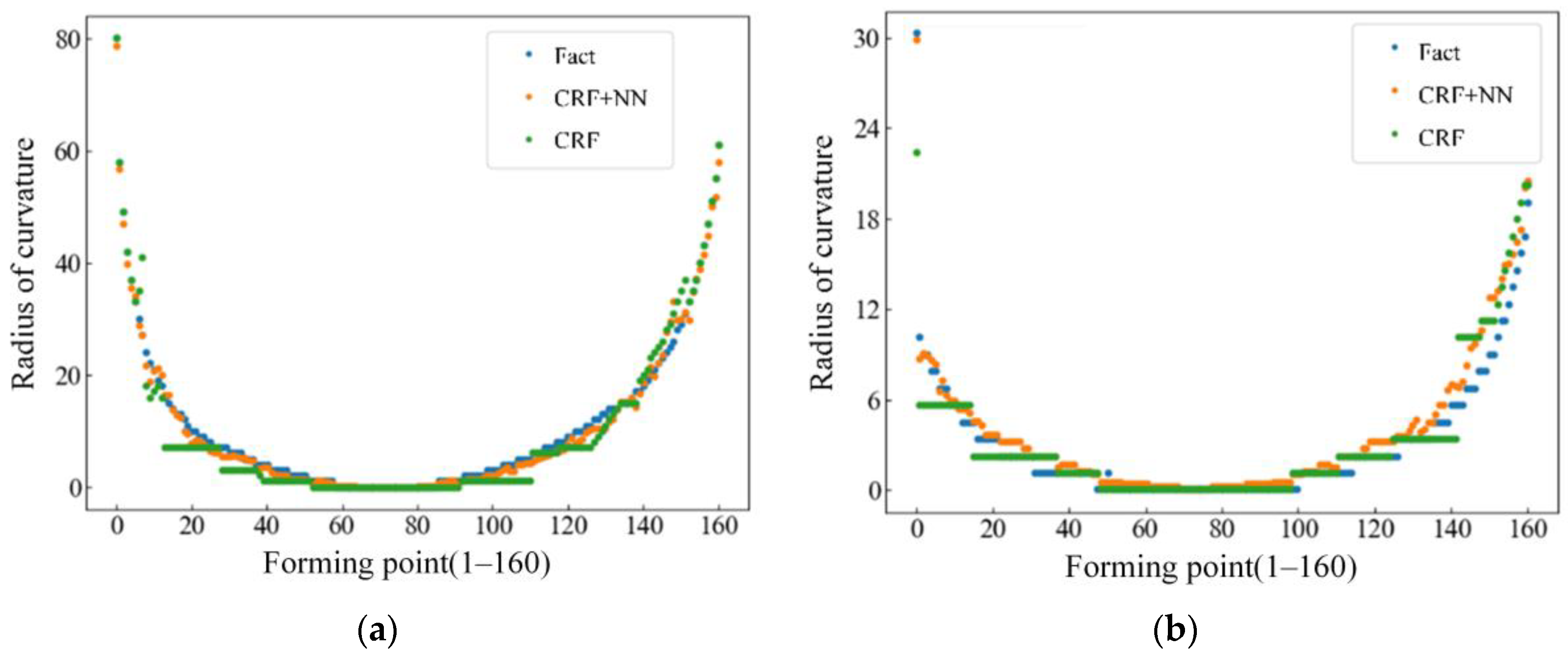
Based on the prediction results of a fixed curvature, a variable-curvature prediction model based on the conditional random field was established, the state transition law of variable-curvature forming was explored, and the accurate prediction of the curvature of the variable-curvature rolling profile was realized. By adding an error compensation network after the result of the conditional random field, the discrete sequence was mapped to the continuous sequence. Table 8 shows the comparison between the MSE, MAE, and MAPE of the prediction results of the two variable-curvature springback prediction models. The MSE, MAE, and MAPE prediction results of the model without an error compensation network are 3.42, 2.12, and 24.30, respectively. The MAE, MSE, and MAPE prediction results of the model with an error compensation network are 1.40, 0.66, and 13.72, respectively. The improvement of model accuracy by adding the error compensation network was shown. A variable-curvature prediction model that can accurately predict the curvature after forming was obtained.

References

1. Tao, J.; Xiong, H.; Wan, B.F.; Wei, W.B.; Cheng, X.; Wang, L.T.; Yu, Y.H.; Wang, C.; Guo, X.Z. 3D Free-bending forming equipment and key technology. J. Netshape Form. Eng. 2018, 10, 1–13. [Google Scholar] [CrossRef]
2. Desinghege, S.G.; Hodgson, P.; Weiss, M. Microstructure effects on the material behaviour of magnesium sheet in bending dominated forming. J. Mater. Process. Technol. 2021, 289, 116951. [Google Scholar] [CrossRef]
3. Su, C.; Liu, J.; Zhao, Z.; Lou, S.; Wang, R.; Yang, L. Research on roll forming process and springback based on five-boundary condition forming angle distribution function. J. Mech. Sci. Technol. 2020, 34, 5193–5204. [Google Scholar] [CrossRef]
4. Wang, Z.; Lin, Y.; Qiu, L.; Zhang, S.; Fang, D.; He, C.; Wang, L. Spatial variable curvature metallic tube bending springback numerical approximation prediction and compensation method considering cross-section distortion defect. Int. J. Adv. Manuf. Technol. 2021, 118, 1811–1827. [Google Scholar] [CrossRef]
5. Fan, L.-F.; Gou, J.; Wang, G.; Gao, Y. Springback Characteristics of Cylindrical Bending of Tailor Rolled Blanks. Adv. Mater. Sci. Eng. 2020, 2020, 9371808. [Google Scholar] [CrossRef] [Green Version]
6. Chang, Y.; Wang, N.; Wang, B.; Li, X.; Wang, C.; Zhao, K.; Dong, H. Prediction of bending springback of the medium-Mn steel considering elastic modulus attenuation. J. Manuf. Process. 2021, 67, 345–355. [Google Scholar] [CrossRef]
7. Sharma, P.K.; Gautam, V.; Agrawal, A.K. Analytical and Numerical Prediction of Springback of SS/Al-Alloy Cladded Sheet in V-Bending. J. Manuf. Sci. Eng. 2021, 143, 031011. [Google Scholar] [CrossRef]
8. Liu, X.-L.; Cao, J.-G.; Huang, S.-X.; Yan, B.; Li, Y.-L.; Zhao, R.-G. Experimental and numerical prediction and comprehensive compensation of springback in cold roll forming of UHSS. Int. J. Adv. Manuf. Technol. 2020, 111, 657–671. [Google Scholar] [CrossRef]
9. Julsri, W.; Sanrutsadakorn, A.; Uthaisangsuk, V. Experimental and numerical study of springback effect of advanced high strength steel in a V-shape bending. IOP Conf. Ser. Mater. Sci. Eng. 2021, 1157, 012042. [Google Scholar] [CrossRef]
10. Wu, J.J.; Zhang, H.G.; Wang, J.B.; Wang, Y.J. Mechanical and spring-back analysis for the stretch-bending process of extruded profile. Mater. Sci. Technol. 2004, 12, 357–359. [Google Scholar] [CrossRef]
11. Choi, H.; Fazily, P.; Park, J.; Kim, Y.; Cho, J.H.; Kim, J.; Yoon, J.W. Artificial intelligence for springback compensation with electric vehicle motor component. Int. J. Mater. Form. 2022, 15, 22. [Google Scholar] [CrossRef]
12. Sun, C.; Wang, Z.; Zhang, S.; Liu, X.; Wang, L.; Tan, J. Toward axial accuracy prediction and optimization of metal tube bending forming: A novel GRU-integrated Pb-NSGA-III optimization framework. Eng. Appl. Artif. Intell. 2022, 114, 105193. [Google Scholar] [CrossRef]
13. Lu, K.; Zou, T.; Luo, J.; Li, D.; Peng, Y. Stretch bending process design by machine learning. Int. J. Adv. Manuf. Technol. 2022, 120, 781–799. [Google Scholar] [CrossRef]
14. Cruz, D.J.; Barbosa, M.R.; Santos, A.D.; Miranda, S.S.; Amaral, R.L. Application of Machine Learning to Bending Processes and Material Identification. Metals 2021, 11, 1418. [Google Scholar] [CrossRef]
15. Liu, S.; Xia, Y.; Shi, Z.; Yu, H.; Li, Z.; Lin, J. Deep Learning in Sheet Metal Bending with a Novel Theory-Guided Deep Neural Network. IEEE/CAA J. Autom. Sin. 2021, 8, 565–581. [Google Scholar] [CrossRef]
16. Xu, B.; Li, L.; Wang, Z.; Zhou, H.; Liu, D. Prediction of springback in local bending of hull plates using an optimized backpropagation neural network. Mech. Sci. 2021, 12, 777–789. [Google Scholar] [CrossRef]
17. Li, L.; Zhang, Z.; Xu, B. Prediction of Spherical Sheet Springback Based on a Sparrow-Search-Algorithm-Optimized BP Neural Network. Metals 2022, 12, 1377. [Google Scholar] [CrossRef]
18. Wasif, M.; Fatima, A.; Ahmed, A.; Iqbal, S.A. Investigation and Optimization of Parameters for the Reduced Springback in JSC-590 Sheet Metals Occurred During the V-Bending Process. Trans. Indian Inst. Met. 2021, 74, 2751–2760. [Google Scholar] [CrossRef]
19. Serban, F.M.; Grozav, S.; Ceclan, V.; Turcu, A. Artificial Neural Networks Model for Springback Prediction in the Bending Operations. Teh. Vjesn.-Tech. Gaz. 2020, 27, 868–873. [Google Scholar] [CrossRef]
20. Trzepieciński, T.; Lemu, H.G. Improving Prediction of Springback in Sheet Metal Forming Using Multilayer Perceptron-Based Genetic Algorithm. Materials 2020, 13, 3129. [Google Scholar] [CrossRef]
21. Liang, Z.; Zou, T.; Dai, W.; Zhang, Z.; Liu, Y.; Lu, K.; Li, D.; Ding, S.; Peng, Y. Compensate for longitudinally discrepant springback and bow in chain-die forming processes by multiple sections optimization. Int. J. Adv. Manuf. Technol. 2022, 121, 6407–6430. [Google Scholar] [CrossRef]
22. El Mrabti, I.; Touache, A.; El Hakimi, A.; Chamat, A. Springback optimization of deep drawing process based on FEM-ANN-PSO strategy. Struct. Multidiscip. Optim. 2021, 64, 321–333. [Google Scholar] [CrossRef]
23. Jia, X.; Gong, H.; Shi, W.; Yang, C.; Yuan, K. Multi-objective Optimization of Forming Quality on High-Strength Steel Rocker Arm Parts. Trans. Indian Inst. Met. 2022, 75, 2661–2671. [Google Scholar] [CrossRef]
24. Akrichi, S.; Abid, S.; Bouzaien, H.; Ben Yahia, N. SPIF Quality Prediction Based on Experimental Study Using Neural Networks Approaches. Mech. Solids 2020, 55, 138–151. [Google Scholar] [CrossRef]
25. Ciubotariu, V.A.; Radu, M.C.; Herghelegiu, E.; Zichil, V.; Grigoras, C.C.; Nechita, E. Structural and Behaviour Optimization of Tubular Structures Made of Tailor Welded Blanks by Applying Taguchi and Genetic Algorithms Methods. Appl. Sci. 2022, 12, 6794. [Google Scholar] [CrossRef]
26. Kong, Q.; Yu, Z. Dynamic Evaluation Method of Straightness Considering Time-Dependent Springback in Bending-Straightening Based on GA-BP Neural Network. Machines 2022, 10, 345. [Google Scholar] [CrossRef]
27. Ji, C.; Lei, Y. Parallel clustering by fast search and find of density peaks. In Proceedings of the 2016 International Conference on Audio, Language and Image Processing (ICALIP), Shanghai, China, 11–12 July 2016; pp. 563–567. [Google Scholar] [CrossRef]
28. Chen, T.; Guestrin, C. XGBoost: A Scalable Tree Boosting System. In Proceedings of the KDD’16: The 22nd ACM SIGKDD International Conference on Knowledge Discovery and Data Mining, San Francisco, CA, USA, 13–17 August 2016; pp. 785–794. [Google Scholar] [CrossRef] [Green Version]
29. Banerjee, I.; Ling, Y.; Chen, M.C.; Hasan, S.A.; Langlotz, C.P.; Moradzadeh, N.; Chapman, B.; Amrhein, T.; Mong, D.; Rubin, D.L.; et al. Comparative effectiveness of convolutional neural network (CNN) and recurrent neural network (RNN) architectures for radiology text report classification. Artif. Intell. Med. 2019, 97, 79–88. [Google Scholar] [CrossRef]
30. Gers, F.A.; Schmidhuber, J.; Cummins, F. Learning to Forget: Continual Prediction with LSTM. Neural Comput. 2000, 12, 2451–2471. [Google Scholar] [CrossRef]
31. Song, R.; Liu, Y.; Zhao, Y.; Martin, R.R.; Rosin, P.L. Conditional random field-based mesh saliency. In Proceedings of the 2012 IEEE International Conference on Image Processing (ICIP 2012), Orland, FL, USA, 30 September–3 October 2012; pp. 637–640. [Google Scholar] [CrossRef]
Figure 1. Schematic diagram of data distribution after clustering.
Metals 13 00143 g001
Figure 2. Fixed-curvature roll-bending forming coupling analyzer training process.
Metals 13 00143 g002
Figure 3. Schematic diagram of XGBoost structure.
Metals 13 00143 g003
Figure 4. Comparison of predicted results with fixed curvature and actual results.
Metals 13 00143 g004
Figure 5. Conditional random field undirected graph model.
Metals 13 00143 g005
Figure 6. Profile discretization data representation.
Metals 13 00143 g006
Figure 7. Variable-Curvature Prediction Input–Output Structure.
Metals 13 00143 g007
Figure 8. Horizontal symmetrical three-roll roll bending machine.
Metals 13 00143 g008
Figure 9. Partially Fixed Curvature Experimental Profiles.
Metals 13 00143 g009
Figure 10. Comparison between the initial model and the model after Bayesian optimization of hyperparameters. (a) Initial hyperparameter combination model effect; (b) Model effect after Bayesian optimization of hyperparameters.
Metals 13 00143 g010
Figure 11. Model Fit Comparison Chart. (a) Polynomial regression; (b) SVR; (c) neural networks; (d) XGBoost + Bayes.
Metals 13 00143 g011
Figure 12. Partially variable-curvature experimental profiles.
Metals 13 00143 g012
Figure 13. Contrast experiment between fixed-curvature model and variable-curvature model. (a) Experiment No.1; (b) Experiment No.2.
Metals 13 00143 g013
Figure 14. Experimental comparison with error compensation network. (a) Experiment No.1; (b) Experiment No.2.
Metals 13 00143 g014