Article

Global Droplet Heat Transfer in Oxygen Steelmaking Process

1
Fluid and Process Dynamics (FPD) Group, Department of Mechanical and Product Design Engineering, Swinburne University of Technology, Hawthorn, VIC 3122, Australia
2
Tata Steel, 1951 IJmuiden, The Netherlands
*
Author to whom correspondence should be addressed.
Metals 2022, 12(6), 992; https://doi.org/10.3390/met12060992
Submission received: 15 May 2022 / Revised: 2 June 2022 / Accepted: 6 June 2022 / Published: 10 June 2022
(This article belongs to the Special Issue Oxygen Steelmaking Process)

Abstract

:
Generated droplets in a basic oxygen furnace (BOF) process create an interfacial area between metal and slag/emulsion that helps in heat transfer during different stages of the blowing period. Previous studies have developed extensive models to understand bloating behavior and overall refining kinetics contributed by the droplets in a BOF process. Except for the recent study on single droplet heat transfer by the current authors, no studies in the open literature have addressed the heat transfer contributed by droplets in a BOF. The present work is an extension of single droplet heat transfer, wherein a global droplet heat transfer model is developed by integrating kinetic and dynamic aspects of generated droplets during the blowing period. The model was developed based on previous chemical kinetic studies and input values from plant trials. The results from the global droplet heat transfer model are integrated into the overall zone heat balance calculations to predict the temperature evolution profile of hot spot, slag, and hot metal zones during the blowing period. The results highlight that the hot spot temperature ranges from 1900 °C to 2090 °C, with a peak value of around 2300 °C observed during the middle of the blow. Furthermore, computing the overall droplet heat transfer efficiency, it was observed that the droplets transfer 90% of the heat to the slag up to the first 10 min of the blow, and then the heat transfer efficiency drops towards the end of the blow.

1. Introduction

In a basic oxygen furnace (BOF), a high-speed oxygen jet creates a cavity on the hot metal bath and generates a large number of metal droplets. The ejected droplets interact with the slag or emulsion zone and fall back into the bath. During the residence time refining action mainly, a decarburization reaction takes place in the slag-gas-metal emulsion zone. A large number of generated droplets facilitates a high surface area for reaction. The study conducted by Rout et al. [1], estimated that more than 75% of de-C takes place during the main blow in the gas–metal–slag emulsion phase. In addition to refining reactions, a larger surface area provides possibilities for heat transfer between metal droplets and the surrounding medium. Therefore, the overall droplet heat transfer can either heat up or cool down the slag/emulsion zone surrounding the droplets. However, previous studies have not discussed the role of droplets in heat transfer for a BOF steelmaking process. The high temperature inside the furnace hinders the direct analysis of the thermal behavior of droplets during the blowing period. Therefore, an overall droplet heat transfer model is required to provide an understanding of the following areas:
(a)
How does the global droplet heat transfer affect the temperature of the participating medium (slag/emulsion zone)?
(b)
What mode of heat transfer is dominant as the droplet interacts with the slag/emulsion zone?
(c)
The influence of droplet heat transfer on the chemical refining of the process.
(d)
The effect of parameters such as droplet size, residence time, porosity(foaming) of surrounding medium on droplet heat transfer.
To understand the BOF process, numerous experimental and theoretical studies have investigated the behavior of droplets in slag–metal–gas emulsions. Previous studies were mainly concentrated on droplet generation [2,3,4,5,6], droplet swelling [7,8,9,10,11,12,13,14], trajectory/velocity and residence time [3,15,16,17,18], temperature of zones surrounding the droplet [1,19,20], refining kinetics [16,17,21,22,23,24,25], CO nucleation, and escape [26]. With the hot model experimental data, Subagyo et al. quantified droplet generation using a dimensionless number, known as the blowing number (NB). A recent study by Rout et al. has considered the effect of ambient furnace temperature and redefined the dimensionless number to a modified blowing number (NB,T). Based on the size distribution analysis, studies [2,15,16,18,21,22,23,27,28] have reported that droplet diameters vary from 0.016 mm to 6 mm. The droplet swelling studies [7,8,9,10,11,12] show that the diameter of the droplet increases due to internal nucleation. Consequently, the bloating behavior of the droplet increases the residence time. The average residence time observed from different plant trials [15,16,17], and experimental studies [3,18] varies from 20 to 80 s. The combined effect of blowing number, size distribution, and droplet swelling help to quantify the total interfacial area between the metal droplet and surrounding medium. The results from the study conducted by Dogan et al. [14] predicted that the interfacial area created due to droplet generation was 100 times greater than the jet impact area. Therefore, the generation of a large number of small droplets provides a significant interfacial area for heat transfer and mass transfer to take place.
Concerning the refining kinetics of the process, different studies [16,17,21,22,23,24,25] have concluded that the total C removal at the metal droplets and slag interface is much higher than at the bulk hot metal and slag interface. The infiltration of droplets and their residence time results in the accumulation of metal in the slag/emulsion phase. These metal droplets undergo decarburization through FeO reduction at the interface, which enhances the refining reactions to a great extent [7,17,21,29]. A recent modelling study by Kadrolkar et al. [26] quantifies the CO formed (in terms of internal, external CO nucleation, and CO escape) as a result of the de-C reaction. From the heat transfer perspective, the droplet is heated due to (a) high temperature of the hot spot zone where droplets are generated and (b) heat from carbon oxidation exothermic reaction. Therefore, the heat generated from CO formation will influence the droplet heat transfer.
One of the implications of the present study is aimed to calculate the instantaneous droplet temperature and droplet heat transfer efficiency (that indicates how much heat droplet transfers to the slag) during different stages of the blowing period. The previous study conducted by Rout [1] attempted to calculate the surface temperature of the droplet in the emulsion zone. The study reported that the droplet temperature is 90 K to 200 K greater than the hot metal bath temperature. However, it was acknowledged that the model was developed with several assumptions without considering rigorous heat balance. In another study conducted for an iron bath reactor by Panjkovic [20], the heat transfer between metal droplets and slag droplets with the gaseous environment was calculated (droplet interaction with other zones was not considered). The model did not calculate the droplet generation rate and is assumed to be a constant value. With an interest to understand the thermal behavior of droplets in a BOF process, Madhavan et al. [30] developed a mathematical model to study the heat interaction of a single droplet (undergoing bloating) with slag. The results were validated against the experimental data of Gu et al. [31]. The current study will be an extension of a single droplet heat transfer study wherein a global droplet heat transfer model is developed to (a) quantify the heat transfer rate by droplets throughout the blowing period, (b) predict the temperature profiles of the hot spot, hot metal, and slag zone temperature with respect to time, (c) understand the effect of different reactions contributing to heat and compare it with the droplet heat transfer, and (d) explore the possibilities of optimizing the process in terms of energy consumption.

2. Methodology

The droplets interact with the different surrounding mediums at different stages of the blowing period. In the initial phase of the blow, generated droplets from the hot spot travel through the gaseous atmosphere and fall back into the hot metal bath. During the mid-blow, the droplet travels through the emulsion zone, undergoing refining action. Once the blowing proceeds towards the final stage, the interaction of droplets will be limited to the slag phase. Therefore, it is required to understand how the large number of droplets generated at different stages of the blowing period undergoes heat transfer with the surrounding medium. However, the complexity linked with the global heat transfer model is attributed to transient parameters, such as droplet velocity, size, density, generation rate, CO formation, CO escape, size distribution, internal heat generation, emissivity, residence time, mass transfer, thermal properties of the medium surrounding the droplet, hot spot temperature and heat transfer coefficients, due to convection and radiation. To tackle this problem, a systematic approach is needed. The complexity of the problem is considered by dividing it into different modules. The methodology used for this research is represented using a flow chart as shown in Figure 1 and the algorithm for the model is given in Figure 2.

2.1. Assumptions

The global droplet heat transfer depends on slag temperature and the slag temperature depends on temperatures of other zones (hotspot and hot metal). Therefore, the model is developed to dynamically carry out heat balance at different zones throughout the blowing period. To execute droplet heat balance along with the zone heat balance, different parameters (velocity, density, radius, CO formation, CO escape, internal heat generation, emissivity, mass transfer, thermal properties of the medium surrounding the droplet, and heat transfer coefficients, due to convection and radiation) need to be considered. Incorporating all the parameters for developing the mathematical model is complicated. Therefore, the following simplification and assumptions considered for developing the complete model are explained below:
1.
The geometry of the droplets is assumed to be spherical.
2.
As the droplets are generated from the hot spot, the droplet initial temperature is the same as the hotspot temperature and is assumed to be uniform.
3.
The internal CO formation results in bloating. During the residence time, CO gas escape from the droplet and has negligible contact time with the surface of the metal droplet. Hence, the presence of gaseous layer surrounding the droplet is neglected.
4.
No incubation period for droplets is considered. In the present model, droplets undergo bloating instantaneously as it goes through the slag-emulsion medium. It must be acknowledged that there is experimental evidence for an incubation period for droplets by Chen et al. [11] but in this study, we are ignoring this aspect to simplify the problem. Future work may incorporate this aspect.
5.
A previous study by Dogan et al. has predicted the flux dissolution (CaO and MgO dissolved) profile for Ciccutti [23] plant data, taking into account the charge addition rate and geometry of particles. This predicted profile is used in the present model for slag temperature calculation.
6.
Scrap melting at the initial phase of the blow affects hot metal temperature. To simplify the complexity, the linear scrap melting profile (where scrap melts and dissolves linearly before 7 min of oxygen blow) predicted by Dogan et al. [14] is assumed for the present calculation.
7.
In Cicuttis’s [23] plant data, sampling data are available from 2 min. Therefore, the present model uses values from 2 min onwards.
8.
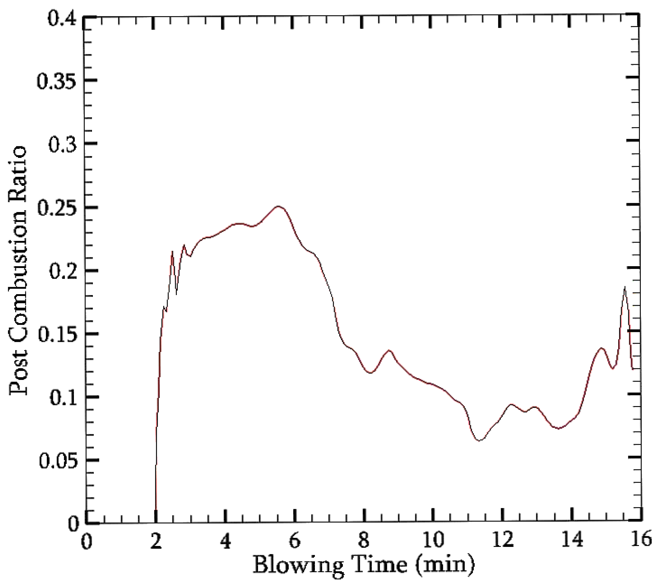
To compute the heat of post-combustion, the PCR profile (post-combustion ratio, defined as the ratio of CO2/(CO + CO2)) is required, which is not recorded in Cicuttis’s [23] plant trial. In the present study, the post combustion profile recorded at Tata steel, the Netherlands is used (given in Appendix A, Figure A1). It is assumed that the post combustion heat will heat up the slag. However, in the actual scenario, there is a possibility that a lot of post combustion heat can escape through the gas stream.
9.
From a heat balance study [32] by the current authors, it was observed that the overall heat loss percentage varies from 2% to 6%. Since heat loss affects the temperature, it is assumed that the an average heat loss value is 3% throughout the blowing period and it happens from the slag zone.
10.
To carry out heat balance at different zones (hotspot, slag, and hot metal), mass evolution and refining profiles are required. For Cicuttis’s [23] plant data, Rout et al. [1], Kadrolkar et al. [33] and Dogan et al. [14] have predicted the hot metal mass, slag mass, and refining profiles. The present model uses these refining profiles for predicting the temperature of respective zones.
11.
To reduce the complexity, the predicted temperature of the slag zone, hot spot zone, and hot metal zone at different stages of blowing are assumed to be uniform.

2.2. Jet Velocity Module

In a BOF, the supersonic jet of oxygen is blown from the lance onto the hot metal bath. Previous studies have developed several empirical correlations to calculate the axial velocity of the supersonic jet impinging a hot metal bath at a distance “h” from the nozzle exit. In the present study, the velocity of the jet is computed using the relation Equation (1) suggested by Sumi et al. [34] based on Ito and Muchi’s [35] jet model.
Velocity of Jet
u j   =   u 0 ·   ( 1 e ( 0.5 ϵ u ) )
ϵ u = α ρ a ρ e h d e β
where u j   is iet axial velocity,   u 0 is nozzle exit velocity, h is lance height, d e is nozzle exit diameter, ρ e is nozzle exit gas density,   ρ g , h is gas jet at the impingement point, ρ a is density of the ambient gas; α , and β are constants with values 0.0841 and 0.6035 obtained from the experiment. The gas velocity at the metal surface is related to the jet velocity expressed using the equation below.
Velocity of Gas
u g = η · u j
where η is the value obtained from experiments for the onset of splashing, which corresponds to a weber number value greater than 10. For a vertical jet impinging on a liquid hot iron bath (with a penetration depth of 2.52 cm), the value of η = 0.4771.

2.3. Jet Temperature Module

The temperature is calculated using the equation for enthalpy H that represents heat at the point of impact of the oxygen jet. The H value for a particular h d e can be calculated by solving the set of equations (Equations (4)–(8)). In a top-blown BOF, CO gas from the de-C can react with the oxygen jet forming CO2. This reaction is known as a post-combustion reaction, which is exothermic in nature and can heat the oxygen jet. However, it needs to be acknowledged that for the jet temperature calculation, the enthalpy of the jet being heated by the post-combustion rection is not considered for the present study. This is because the post-combustion reaction is heterogeneous and unsteady in nature with the flow conditions. Therefore, a module that couples aspects of fluid dynamics with the kinetics of chemical reactions and thermodynamics is required to calculate the influence of post-combustion on jet temperature. In the present study, a simplistic approach is used to calculate the enthalpy at the impact point.
Enthalpy at Impact point
H = ( H o H a ) H m + H a
H m = ( 1 e ( 0.5 ϵ h ) )
ϵ h = α P r ρ a ρ e h d e β
Ho is the ambient enthalpy.
H o = C p _ o · T o + u j 2 2
He is the enthalpy of gas at the nozzle exit.
H a = C p _ a · T a + u j 2 2
The temperature of the gas jet is T g at a distance h from the nozzle exit.
T g = H u j 2 C p
Once the temperature is calculated, the density of the gas jet at the impact point is computed using the following ideal gas equation:
ρ g , h = P a M O 2 R T g

2.4. Hot Spot Temperature Module

The point where the supersonic jet impinges the hot metal bath generates high heat, resulting in the maximum temperature inside the furnace. A typical hot spot temperature reported from different studies ranges from 1850 K to 2500 K [36,37,38,39]. As the droplets are generated from the hot spot zone, the initial temperature of the droplet will be the same as the hot spot temperature. A recent study by Rout et al. [1] has computed the refining profiles at the hot spot zone using Ciccutti’s plant data [23]. In the present study, the temperature of the hot spot is calculated using Equation (16), considering the predicted refining profile by Rout et al. [1]. At the hot spot, the heat generation Qreaction is contributed by decarburization, silicon oxidation, and iron oxidation reactions. Simultaneously, the heat is transferred to the bath (Qbath) and flue gas (Qgas) side from the hot spot zone, as shown in Figure 3. Therefore, the heat balance can be written as the following equation:
Q r e a c t i o n   = Q b a t h + Q g a s
Q r e a c t i o n   = m C O · H C O + m S i O 2 · H S i O 2 + m F e O · H F e O
Q b a t h = h b · A h s · ( T h s T b )
Q g a s = h g · A h s · ( T h s T g )
A h s = π · d c 12 · h c 2   [ ( d c 2 4 + 4 · h c 2 ) 1.5 d c 3 8 ]
h c h = 4.469 · [ 0.7854 × 10 5 · d t · P a · ( 1.27 P o P a 1 ) cos α · 1 g ρ l h 3 ] 0.66
d c h = 2.813 · [ 0.7854 × 10 5 · d t · P a · ( 1.27 P o P a 1 ) · ( 1 + sin α ) · 1 g ρ l h 3 ] 0.282
T h s = Q r e a c t i o n   + h b · A h s · T b + h g · A h s · T g h b · A h s + h g · A h s
where T h s is the temperature at the hot spot, A h s is the surface area of the hot spot, h b and h g are the heat transfer coefficients from hot spot to bath and gas, respectively, d c and h c are the height and depth of the cavity. In Asai et al.’s [40] study, the values used for h b and h g were estimated as 50,000 W/m2.s. °C and 2500 W/m2.s. °C. Similarly, the surface area of the hot spot cavity is expressed by the equation Equation (15) based on Urquhart’s study [41]. In the Equation (16), Equation (17) the depth and diameter of the hot spot cavity are calculated using the dimensionless relation proposed by Koria and Lange [42].

2.5. Droplet Generation Module

The droplet generation rate is calculated as a function of a dimensionless number called a blowing number. This number represents the surface instability due to thr gas jet interaction with the hot metal bath by considering gravity, inertia, and surface tension forces. A recent study by Rout et al. [6] has modified the blowing number equation formulated by Subagyo et al. [4] by considering the effect of temperature on the forces. The modified blowing number is given by the Equation (19). Similarly, the volumetric flow rate (in cubic meters per minute) is also corrected against the gas jet temperature and pressure and is expressed using the Equation (20). Linking Equations (19) and (20) to the empirical relation Equation (21), the amount of droplets generated in kilogram per minute is computed.
N B , T = η 2 ρ g , h u j 2 2 σ l ρ l g
F G , T =   P N T P P h · T g T N T P   F G
R B , T F G , T = N B , T 3.2 ( 2.6 × 10 6 + 2.0 × 10 4 · ( N B , T ) 12 ) 0.2

2.6. Droplet Size Distribution Module

From the heat transfer perspective, the droplet generation rate, as well as the size distribution of the droplets, plays a vital role. The size distribution of the droplet has a direct relation to the interfacial area that facilitates heat transfer. In the present study, the size distribution was calculated using Rosin–Rammler–Sperling (RRS) distribution function [4,27].
R s = 100 ·   exp   ( d d ) n
where Rs is a measure of the screen oversized with diameter d, n is the size distribution homogeneity; d′ is the measure of fitness. Values of n and d′ are 1.75 and 1.26, respectively [4,14]. From Cicutti’s [23] plant study, the total range of droplet sizes was found to vary from 0.23 mm to 3.35 mm.
Considering the different sizes of droplets generated at the same time results in calculation complexity. Therefore, in the present study, it is assumed that all droplets generated are of an initial diameter of 2.5 mm. We believe it is a justifiable assumption as a starting step to understand the global droplet heat transfer but future studies may explore this aspect.

2.7. Droplet Velocity Module

Initial Velocity

The kinetic energy of the oxygen jet imparts energy to the hot metal bath. This energy results in droplet generation and ejects droplets from the surface of the hot metal bath. According to Subagyo et al. [4], the initial velocity of the droplet can be estimated through the energy conservation relationship given by the equation. In addition, the kinetic energy of the droplet E k d and the blowing gas E k g are calculated by using equations Equation (24) and Equation (25), respectively.
E k d E k g = 1.43 × 10 3 · N B , T 0.7
E k d = 1 2 · R B , T u d 0 2  
E k g = 1 2 · ρ g , h   Q O 2   u g , h 2 = N B , T   Q O 2 σ l ρ m g
By combining and rearranging equations, the initial velocity of the droplet is calculated by the following equation:
U d o   = 2.86 × 10 3 · N B , T 0.7 · E k g R B , T

2.8. Instantaneous Velocity

The ejected droplet travels through different surrounding mediums (as discussed in Section 2) at different stages of the blowing period. Therefore, the velocity of the droplet will be influenced by the forces exerted by the surrounding medium. Considering a ballistic trajectory, the previous study conducted by Subagyo et al. [43] and Brooks et al. [13] uses force balance and expressed horizontal and vertical components of velocity using Equations (27) and (28). The differential equation is discretized using the simple explicit forward differencing method (Equations (35) and (36)). The net resultant of the horizontal and vertical components quantifies the instantaneous velocity of the droplet given by Equation (37).
d U r d t = ρ s l a g · C D , r t ρ s l a g + 2 ρ D t A p t   V D t U r 2 A p t = π D d t 4
d U Z d t = 2 ( ρ s l a g ρ D t ) · g ρ s l a g + 2 ρ D t ρ s l a g ·   C D , Z t ρ s l a g + 2 ρ D t   A s t   V D t   · U z 2
Simplification
K o   = 2   ( ρ s ρ   d ) g ρ s + 2   ρ   d                              
K z   = 3   ρ s C D , z 2 ( ρ s + 2   ρ   d ) D d                                   w h e n   ( U z > 0 )
K z   = 3   ρ s C D , z 2 ( ρ s + 2   ρ   d ) D d                                         w h e n   ( U z < 0 )
K r   = 3   ρ s C D , r 2 ( ρ s + 2   ρ   d ) D d  
d U r d t = K 0 + K z u z 2
d U r d t = K r u r 2
Discretization (simple explicit forward method)
U Z t U Z t 1 t = K 0 + K z t 1 u z t 1 2
U r t U r t 1 t = K r t 1 u z t 1 2
U D t = U r t 2 + U Z t 2

2.9. Bloating and Diameter Change Module

One of the highlighted aspects of the droplet generated in a BOF process is the bloating phenomenon. The CO formation within the droplet results in the droplet bloating. As a consequence, the area, volume, and density of the droplet change. These parameters are related to the decarburization rate r c . The decarburization rate is expressed using the first-order reaction rate principle given by Equation (38) [13]. The critical decarburization rate can be evaluated by the empirical relation Equation (39) suggested by Brooks et al. [13], based on the experimental study of Molloseau and Fruehan [24].
r c = K e f f A D t V D t ·   ( % C % C e )
r c * = {   2.86 × 10 6 × ( w t % F e O ) ,     % F e O < 20 2.86 × 10 6 × 20 ,     % F e O 20
where % C is the weight percentage carbon content in the droplet, % C e is the equilibrium weight percentage of carbon content, K e f f is the effective rate constant (m/s); A D t and V D t are the surface area (m2) and volume (m3) of the droplet. Subsequently, the influence of decarburization rate on the apparent density ρ d of the droplet is calculated through the following Equation (40):
ρ d   = {       ρ d o   r c * r c ,           i f   ( r c > r c * ) ρ d o ,             i f   ( r c r c * )
where ρ d o is the initial droplet density (kg/m3). Assuming the generated droplets are spherical in shape, the radius of the droplet at each instant of time is calculated by the following equation:
r D t = ( 3 4 π · m D t ρ d ) 3

2.10. Droplet Trajectory and Residence Time Module

To trace the ballistic motion of the droplet, instantaneous trajectories Lr (horizontal direction) and Lz (vertical direction) are calculated by integrating Ur and Uz given by Equation (42) and Equation (43), respectively. Furthermore, the residence time represents the instant the droplet falls back into the hot metal bath, i.e., the Lz becomes zero. Therefore, the residence time is the “t” value corresponding to the condition given by the Equation (44).
L z = 0 t U z · d t
L r = 0 t U r · d t
L z = 0 t U z · d t = 0

2.11. Instantaneous Droplet Heat Transfer Coefficient Module

As the droplet undergoes a ballistic motion, it exchanges heat with the surrounding medium (slag or emulsion based on the stages of the blowing period) through convection and radiation. With the change in temperature and velocity of the droplet and temperature of the surrounding medium, the heat transfer coefficients vary. The convective heat transfer coefficient is calculated based on the Nusselt number relation Nu . For the spherical shape of the droplet, the Nusselt number relation corresponding to a completely submerged sphere moving in a fluid (either liquid or gas or both) medium needs to be selected. The previous experimental studies [44,45,46,47] have obtained various empirical relations for the Nusselt number for a similar case. However, the relation proposed by Ranz and Marshal [45] (Equation (46)) is closely related to the present study to compute the convective heat transfer coefficient h c . The calculation of reynolds number and prantl numer is discussed in the single droplet heat transfer study [30]. To compute the radiative heat transfer coefficient h r , the emissivity and temperature of both the surrounding medium and droplet are required. The previous study [20] on droplet heat transfer in an iron bath reactor calculates the radiative heat transfer coefficient by assuming droplets as a grey body and emissivity independent of temperature and wavelength. With a similar approach, the radiative heat transfer coefficient is expressed by Equation (47).
h = h c + h r
Nu = 2 + 0.58   Re 1 2   Pr 1 3
h r = σ T s l a g 3 1 ε D + 1 ε s l a g 1 [ 1 + T D T s l a g + ( T D T s l a g ) 2 + ( T D T s l a g ) 3 ]
where h represents the overall heat transfer coefficient (W/m2K), σ is the Stefan Boltzmann constant (W/m2K4); ε D , ε s are the emissivity of the droplet and surrounding medium, respectively.

2.12. Single Droplet Heat Balance Module

In the single droplet heat balance module, each droplet of different classes is considered, and the heat balance is studied. As the droplet size (diameter) varies from 0.23 mm to 3.35 mm [23], the preliminary step is to identify the category of heat transfer analysis that this problem belongs. The two main categories are (a) lumped heat capacitance model subjected to convection and radiation; (b) transient heat transfer model with boundaries interacting via convection and radiation. In the lumped system, the temperature of the droplet is a function of time. Whereas, in the latter one, the temperature of the droplet is a function of time and radius. The criteria to check the category is based on the value of the biot number given by the Equation (48). For the value of the biot number 0.1, the heat transfer problem belongs to the category of the lumped system. On the other hand, the problem is solved via a transient heat transfer approach.
Bi =   h · r D t k D
where the value of h depends on the droplet motion, thermal properties of the participating medium (slag/emulsion), and porosity or foam factor. Therefore, the current study calculates the mentioned properties based on the chemistry of the slag/emulsion observed from Ciccutti’s [23] plant data. The analysis shows that for a Biot number equal to 0.1, the diameter of the droplet should be 8.5 mm, which is greater than the droplet sizes considered for the present study. Hence, the lumped capacitance approach is used in the model to predict the droplet temperature from a single droplet heat balance module.
Q ˙ = Q C ˙ + Q R ˙ + Q ˙ G e n
Q ˙ = m D t C p , D d T D d t r
Q C ˙ = h c A s t ( T s l a g T D )
Q R ˙ = h r     A s t   ( T s l a g T D )
Q ˙ G e n = Q C O f o r m a t i o n = m C O f o r m a t i o n · Δ H CO
Governing Equation
m D t · C p , D t d T D d t = h c A s t ( T D T s l a g ) + h r     A s t   ( T s l a g T D ) + Q ˙ G e n
d T D d t = ( h c + h r ) ·   A s t m D t · C p , D t ( T s l a g T D ) + Q ˙ G e n m D t · C p , D t
Discretized Governing Equation
T D t + 1 T D t t = (   h c i t + h r i t ) ·   A s t m D t · C p , D t ( T s l a g T D t ) + Q ˙ G e n m D t · C p , D t
Initial Condition
T ( 0 ) = T H o t s p o t  
With the calculated temperature, the heat transfer Q ˙ D between the metal droplet and the slag is obtained by Equation (58). In addition, the heat transfer efficiency of the droplet from each class at different stages of blowing is computed via the following Equation (59). The heat transfer efficiency will represent the capability of a droplet to transfer heat with the participating medium (slag/emulsion) during one complete circulation period (from ejection time until it returns to the bath) compared to the maximum heat transfer.
Q ˙ D = m ˙ D C p ,   D ( T D , t r ˙ T D , t = 0 ˙ )
η i d ˙   = T D , t r ˙ T D , t = 0 ˙ | T ˙ M e d T D , t = 0 ˙ |
where T D , t r ˙ , T D , t = 0 ˙ are the final temperature and initial temperature of the droplet, and   T ˙ M e d is the temperature of the participating medium (slag/emulsion).

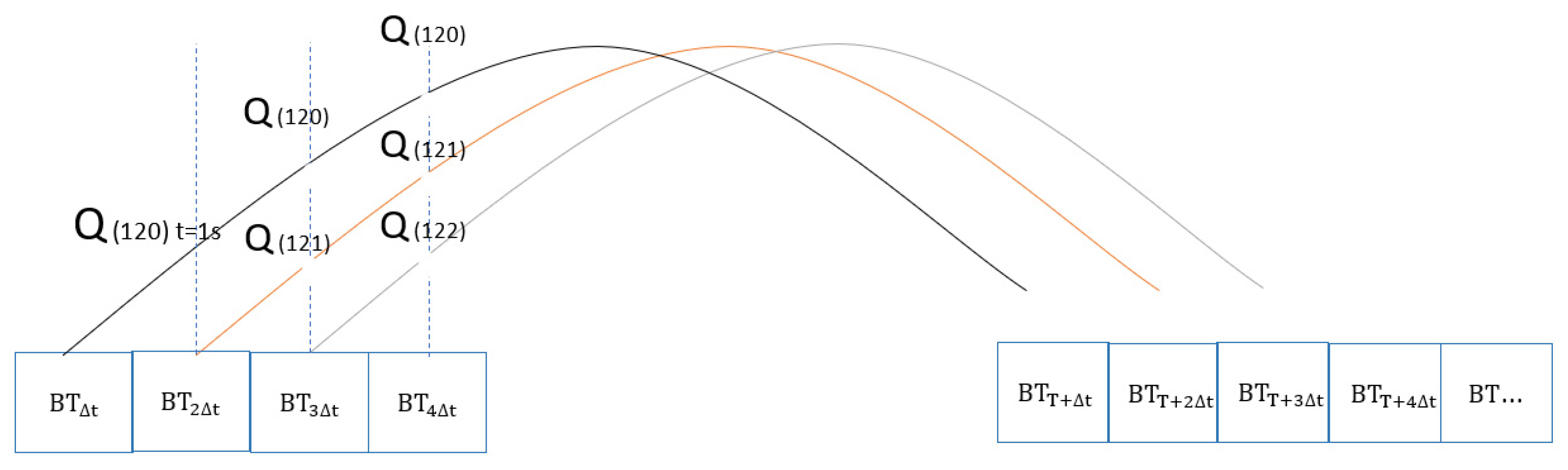
2.13. Overall Droplet Heat Transfer Module

To calculate the overall heat transferred by the droplets to the slag, it is required to consider the total count of droplets at each instant of time. With the droplet generation rate and size distribution, the total number of droplets for each class can be calculated. However, at each instant of the blowing time T b t , the droplets generated from the previous time steps also transfer heat with the surrounding. A schematic diagram to understand the overall droplet heat transfer calculation for an ejected droplet diameter of a single class is shown in Figure 4. The time step for the blowing period in Figure 2 is taken as 1 s and the time step to calculate the droplet velocity is 0.001 s. It is assumed that the calculation starts from a blowing period of 2 min (120 s).
In the practical scenario, the different droplet sizes with the corresponding droplet count will be ejected from the hot metal bath. Considering the droplet count for different classes as n i , a sample formulation to calculate heat transfer at different blowing times is given by the following series of equations (Equation (60)). For example, if the time step is 1 s, then Q 120 , d i t = 1   represent the heat transfer by a droplet of ith class, with a diameter d i that is ejected at a blowing time of 120 s and has travelled for a time step of t equals 1 s ( t = 1 ).
Q 121 = i = 1 10 n i   Q 120 , d i t = 1        
where i is the class of droplet, n i is the count of droplets in ith class; d i is the diameter of droplets in ith class.
Q 122 = i = 1 10 n i   ( Q 121 , d i t = 1   +   Q 120 , d i t = 2 )
Q 123 = i = 1 10 n i   ( Q 122 , d i t = 1 + Q 121 , d i t = 2 + Q 120 , d i t = 3 )
Q 150 = i = 1 10 n i   ( Q 149 , d i t = 1   + Q 148 , d i t = 2 + Q 147 , d i t = 3 Q 122 , d i t = 28 + Q 121 , d i t = 29 )
For the time step of t , the overall droplet heat transfer to the slag Q T b t can be written as the following equation:
Q T b t = i = 1 10 n i   ( Q T b t t , d i t = t + Q T b t 2 t , d i t = 2 t   + Q T b t 3 t , d i t = 3 t + Q ( T b t ( r e s   t i m e ( i ) t ) ) , d i t = r e s   t i m e ( i ) t )
The generalized expression for calculating the overall droplet heat transfer to the slag can be is given by the following equation:
    Q T b t = i = 1 10 n i t i = 1 R Q ( T b t t i · t ) , d i t = t i · t R = r e s   t i m e ( i ) t t
where r e s   t i m e ( i ) is the residence time of droplet in ith class; t i is the each time instant during the residence time of droplet of ith class.
η O = Q D S l g Q D S l g + Q D H M
where η O is the overall droplet heat transfer, Q D S l g and Q D H M are the overall heat transfer by droplets to slag and hot metal.
The current simulation was started after 2.2 min of the blow, as the plant data for the composition of slag and metal (Cicutti [23]) are available after this time. Once the step size was selected, the dynamic process variables, such as lance height, oxygen flow rate, bottom blowing rate, were given as inputs to the model at each numerical time step by the use of several predefined functions, derived from the operational converter data. In the current work, a time step size of 1 s (in the blowing time domain) was chosen for the numerical calculation, as chosen by Dogan et al. [14] and Rout et al. [6].

3. Slag Temperature Module

This module computes the evolution of the slag temperature profile considering different components that contribute heat transfer to the slag/emulsion zone. The temperature is obtained from the slag heat balance. The heat balance is conducted with the slag mass profile captured from Cicutti’s [23] plant data. The different heat components in the slag emulsion zone are as follows:
1.
Heat associated with the oxidation of components in the slag emulsion ( Q ˙ S i , M n ) ;
2.
Heat contributed by droplets generated from the hotspot ( Q ˙ T b t );
3.
Heat for flux dissolution ( Q ˙ F l u x   d i s s );
4.
Heat transfer between slag and bath ( Q ˙ S l g H M );
4.
Heat of post-combustion ( Q ˙ P C );
5.
Heat loss ( Q ˙ H e a t   l o s s ).
m s l g · C p s l g d T s l g d t   = Q ˙ S i , M n + Q ˙ T b t + Q ˙ P C Q ˙ F l u x   d i s s Q ˙ S l g H M Q ˙ H e a t   l o s s
This is schematically shown in Figure 5. The heat associated with the oxidation of the components and flux dissolution are computed based on the profiles predicted by previous studies [1,14,33] for the input condition of Cicutti’s [23] plant data. In the present model, it is assumed that heat loss occurs only from the slag zone. The heat loss value ( Q ˙ H e a t   l o s s ) is obtained by considering 3% of the total heat generated [32] at the slag zone at each instant. The component that transfers heat from slag to bath is quantified using the following formula:
Q ˙ S l g H M = h s h m · A s h m · ( T s T h m )
where the value of h s h m is 80,000 W m 2 K [48] and A s h m is calculated by considering the furnace radius as 3 m. In the current model, this component links the slag zone temperature with the hot metal zone.

4. Hot Metal Temperature Module

The hot metal zone in a BOF process is heated up during the course of blow due to heat transfer from the hot spot to the hot metal ( Q ˙ b a t h ), the slag to the hot metal ( Q ˙ S l g H M ) and droplets returning to the bath ( Q ˙ D H M   ). On the other hand, the heat is simultaneously absorbed in the hot metal zone, due to scrap melting Q ˙ S c r a p for which the linear scarp melting profile predicted by Dogan et al. [14] is considered. With these parameters, the hot metal temperature is computed. This is given by the following equation:
m H M · C p H M d T H M d t = Q ˙ b a t h + Q ˙ D H M   + Q ˙ S l g H M Q ˙ S c r a p
where Q ˙ b a t h is calculated using Equation (13) and Q ˙ D H M from the Equation (70), which is as follows:
Q ˙ D H M   = R B , T · C P D   · ( T D T h m )

5. Algorithm

The algorithm describing the global droplet heat transfer coupled with zone heat transfer is shown in Figure 2.

6. Result and Discussion

The model is developed as per the algorithm and the results are predicted to understand how heat transfer takes place across different zones in a BOF converter. The numerical study was carried out using the plant trial data from Ciccuti et al. for a 200 ton BOF converter. The present study uses the initial input data of Ciccutti et al. [23] and the time-dependent thermal properties of the slag, hot metal, and droplets are calculated based on the empirical relations proposed by Mills [49]. From a thermal analysis perspective, calculating the heat transfer coefficients for a highly dynamic process such as BOF is challenging. This is due to the lack of Nusselt number relations available for the BOF operating conditions. Therefore, the heat transfer coefficients values (hb, hg, hslg-HM) were used from the previous studies, but the hb values were fine-tuned to match the model prediction of the hotspot temperature with the industrial hot spot temperature. It would be preferable to not use this approach for the heat transfer coefficient to the bath but we currently lack enough data to fully calculate this parameter.

6.1. Hot Spot Temperature

In the hotspot, the heat is generated due to the reaction of the oxygen jet with the hot metal impurities. The study conducted by Rout et al. predicted the refining profiles of Si, Mn, and C at the hot spot and another study by Kadrolkar predicted the FeO generation at the hot spot. Using these data, the present model predicted the hot spot temperature profile as shown in Figure 6. The hot spot temperature increases with the blowing time and reaches a peak value of 2300 °C by the middle of the blow. The hot spot temperature was calculated for different sets of heat transfer coefficients. The bath heat transfer coefficient value suggested in the paper by Asai et al. [40] was 50,000 W/m2 K. However, for a heat transfer coefficient value of 50,000 W/m2 K, the hot spot temperature was found to be underpredicted compared to the experimental data recorded by Chiba et al. [50]. Therefore, the present study carried out a calculation with different values of heat transfer coefficient. For a hot metal bath heat transfer coefficient value of 33,400 W/m2 K, the predicted hot spot profile shows a similar trend to that of industrial measured values. Hence, the value of hb assumed for the entire calculation is 33,400 W/m2 K. The predicted hotspot temperatures were assigned as the initial droplet temperature for the generated droplets in the global droplet heat transfer model.

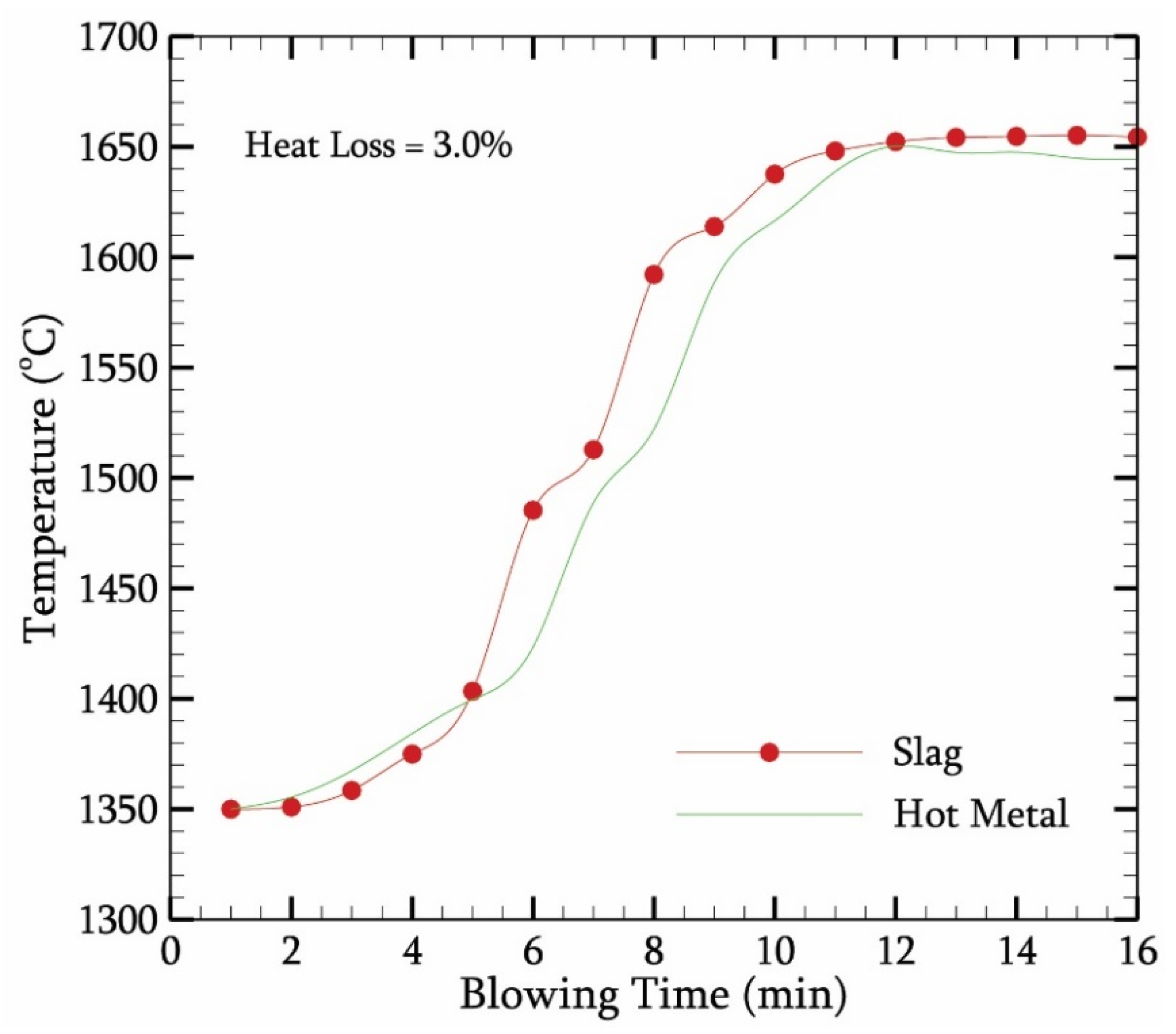
6.2. Slag and Hot Metal Temperature

The heat transferred from the droplets to the slag results in a change in slag temperature. In addition to the droplet heat transfer, an exothermic reaction, such as post-combustion, silicon oxidation, and manganese oxidation, heats the slag. Taking into account all the heat, the slag temperature is predicted as shown in Figure 7. During the initial phase of the blow, the predicted slag temperature is lower compared to the hot metal temperature. The cooling down of the slag temperature is due to the flux dissolution. The temperature of the slag then dominates from the middle of the blow. The slag temperature increase is contributed by the increase in hotspot temperature and de-C reaction taking place in the droplet. In addition, the post combustion heat transfer through the slag-off gas interface will also heat the slag zone. However, a high slag temperature favours the P reversion, which is not beneficial from a refining perspective.
In the case of hot metal, the heat components, such as the heat of the hotspot, convective heat transfer through the slag–hot metal interface, and heat of droplets returning to the hot metal bath contribute to the rise in hot metal temperature, of which the heat transfer via the hot spot contributes the most. Figure 7 shows that until 5 min of the blow, the predicted hot metal temperature is greater than the slag temperature. This is due to the influence of the larger hot spot–hot metal interface area at the initial stage of the blow, afterwhich with the change in lance position, the hot spot–hot metal interfacial area decreases. The current prediction shows that at the end of the blow, the slag temperature (1654 °C) was observed to be 8 °C greater than the hot metal temperature for a constant heat loss of 3%. The calculation were also carried out for different percentages of heat losses and it was found that when the heat loss percentage is changed from 3% to 6%, the slag and hot metal temperature drops by 6 °C.
The numerical study conducted by Huber et al. [51] has predicted the temperature evolution profiles of slag, steel, and PC flame by considering a similar the post-combustion ratio to that of the present study. It is predicted from the study that in the initial phase of the blow, the slag temperature is lower than the hot metal temperature. The slag temperature then becomes greater than the hot metal temperature by the middle of the blow and becomes equal to the hot metal temperature by the end of the blow. The developed model by Huber et al. was tested at ArcelorMittal Dunkerque. However, the details of the model are not mentioned in the literature. The present study also predicts the same trend for the temperature profiles during the blow.

6.3. Effect of Individual Heat Components on Slag Temperature

Unlike the hot metal zone, the evolution of slag zone temperature is due to the cumulative effects of heat components, such as droplet heat transfer, post-combustion heat transfer, and exothermic reaction of silicon and manganese oxidation. Therefore, the influence of individual components on slag temperature considering the heat of flux dissolution, convective heat transfer, and heat loss is shown in Figure 8. The three graphs are obtained by solving the following Equations (71)–(73) using the finite difference method.
Heat Of Droplets
m s l g · C p s l g d T s l g d t = Q ˙ T b t Q ˙ F l u x   d i s s Q ˙ S l g H M Q ˙ H e a t   l o s s
Heat of Post-Combustion
m s l g · C p s l g d T s l g d t = Q ˙ P C Q ˙ F l u x   d i s s Q ˙ S l g H M Q ˙ H e a t   l o s s
Heat of Si, Mn Reaction
m s l g · C p s l g d T s l g d t = Q ˙ S i , M n Q ˙ F l u x   d i s s Q ˙ S l g H M Q ˙ H e a t   l o s s
The predicted profiles show that the droplet heat transfer component has a significant effect. This is because droplets are generated from the hotspot and the de-C reaction adds further heat to the slag. In the case of slag heating by post-combustion, the temperature rise was observed to around 170 °C by the end of the blow. It needs to be highlighted that the slag temperature rise of 170 °C is predicted for a post-combustion ratio of 0.12. Therefore, higher post-combustion can further increase slag temperature. For the oxidation of Si and Mn, the slag temperature was found to be approximately 120 °C. Even though the silicon oxidation is equally exothermic when compared to the post-combustion reaction, the lower mass percentage of silicon in hot metal compared to the C mass percentage results in a lower slag temperature rise.

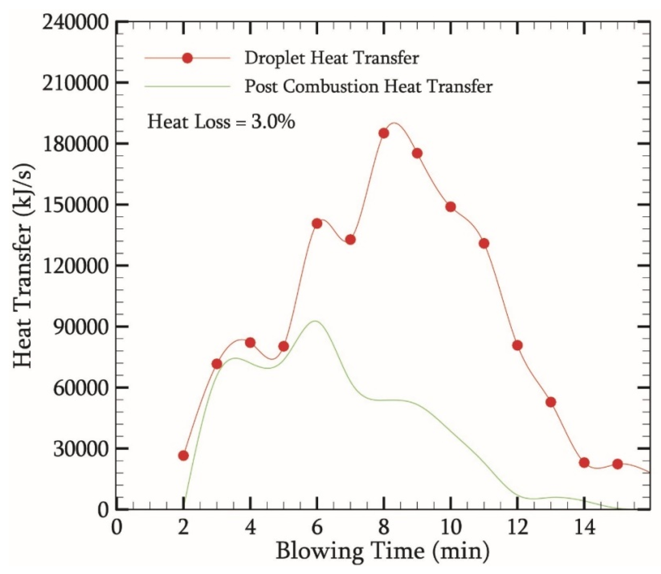
6.4. Heat Transfer Rate via Droplets and Post-Combustion

In the current study, it was observed that the slag generated during the blowing period is mainly heated up by the following two components: (a) heat transferred by droplets; (b) heat due to post-combustion. Figure 9 quantifies the contribution of heat from the respective components. The droplet heat transfer represents the heat transferred by the droplets to the slag. The heat of the droplet is greater than the slag due to (a) droplets being generated at the hot spot and (b) CO generation during the residence time heat the droplets. The peak of droplet heat transfer is observed to be around 8 min. This is due to the fact that de-C reaches a maximum at the same time. During the second half, the droplet heat transfer decreases due to a decrease in the de-C rate and residence time. The dip in the droplet heat transfer profile observed at 5 min and 7 min is due to the change in lance height that influences the droplet generation rate.
The post-combustion heat transfer represents the heat transferred by the post-combustion reaction (CO + 0.5 O → CO2) to the slag. This heat component is calculated by assuming (a) the post-combustion ratio of 0.12 (based on analyzing 35 heat sets from Tata Steel plant data); (b) CO2 is formed at the same instant at which the de-C takes place. Therefore, the maximum heat due to post-combustion was also observed to be around 8 min. It needs to be highlighted that directing the post-combustion heat to the slag is still a topic for research. However, if technologies can aid in directing higher post-combustion heat (through increased post-combustion ratio) to the slag then the BOF process can retain much heat within the converter.

6.5. Droplet Diameter on Slag Temperature

In a BOF, the generated droplet diameter varies from 0.23 mm to 3.35 mm. The diameter and count of the droplet generation influence the refining action. Likewise, the heat transfer is also affected by the size of droplets. As a preliminary step to understand the effect of global droplet heat transfer, the present study assumes that all the droplets generated are of the same size. Figure 10 gives the effect of droplet diameter on slag temperature. With the increase in droplet size, the effect of heat transfer is reduced, resulting in the slag temperature to decrease (as shown in Figure 10a), which in effect decreases the hot metal temperature (as shown in Figure 10b). This is due to the fact that the effective surface area generated by smaller droplets is greater than the larger droplets. Therefore, in further studies, the distribution of droplets will be accounted for to precisely understand the effect on slag temperature due to global droplet heat transfer.

6.6. Droplet Heat Transfer Efficiency

The droplet heat transfer efficiency is a function of droplet residence time in slag. The residence time of droplet generated varies from 20 to 80 s. An increased residence time allows more time for droplets to interact with the slag. The increased residence time is due to the de-C reaction that generates CO gas within the droplets. Once the blowing time crosses 11 min, the rate of de-C decreases. Thus, the residence time of the droplets decreases. The droplet heat transfer efficiency is defined as the heat transferred by the droplets to the slag to the total heat transferred by droplets (to slag and hot metal). Therefore, an increased residence time in the first half of the blow allows for more heat transfer, resulting in higher overall droplet heat transfer efficiency, as shown in Figure 11. In other words, the effect of the slag being heated up by the droplets will be more than the droplets heating the hot metal. However, near the end of the blow, the droplets’ heat transfer to the slag drops due to the decreased residence time of the droplets. Therefore, the overall droplet heat transfer efficiency decreases towards the end of the blow.
In general, the global droplet heat transfer model coupled with the zone heat balance was found to logically explain how the heat flow takes place during the blowing period within the BOF converter. However, the findings from the current study raise different questions, which are as follows:
(a)
How does the assumption of all generated droplets of the same size will significantly affect the slag temperature and hot metal temperature?
(b)
Are there better ways to calculate the different heat transfer coefficient values considering the BOF operating condition?
(c)
From a refining perspective, is it beneficial or not to increase the post-combustion ratio (because higher PCR increases the slag temperature that favours P reversion)?
(d)
How reliable is the assumption from the previous study [26] that FeO is formed only in the hot spot zone? How does it affect heat transfer between different zones?
(e)
The industrial measurements of slag and hot metal temperature evolution profiles are not available in the open literature. So, what are the possibilities of validating the slag and hot metal temperature profiles from the heat transfer model?
To successfully execute the global droplet heat transfer model, the results of the refining profiles from the kinetic studies are required. Therefore, the present model is developed based on the previous studies of Dogan et al. [14], Rout et al. [1], and Kadrolkar et al. [33] that use the input data from the industrial trials conducted by Ciccutti et al. [23]. The predictions from the present model provide a logical starting step to understanding the in-depth aspects of the heat transfer process. However, the values may have deviations compared to the actual scenario. The authors believe that the weaknesses of the present model can be refined by addressing the assumptions and validating the results with more industrial measurements. This will be the basis for future studies.

7. Conclusions

The following conclusions can be drawn from the present study:
  • The predicted hot spot temperature profile shows a similar trend to that of the industrial measured values and a bath heat transfer coefficient value of 33,400 W/m2 K.
  • The slag temperature was predicted to be lower than the hot metal temperature at the initial phase of the blow and thereafter, the slag temperature becomes greater than the hot metal temperature.
  • The modelling work predicts that the effect of droplets heating up the slag is prominent compared to the exothermic heat and post-combustion heat components.
  • Droplets with smaller diameters were predicted to be more effective in heating the slag compared to those with large diameters, as the smaller diameter droplets offer a larger surface area.
  • The calculated droplet heat transfer efficiency shows that until 10 min of the blow, the droplets transfer 90% of the heat of droplets to the slag, and then this declines towards the end of the blow.

Author Contributions

Conceptualization, N.M. and G.A.B.; methodology, N.M.; software, N.M.; validation, N.M.; formal analysis, N.M., G.A.B. and M.A.R.; investigation, N.M., G.A.B. and B.K.R.; resources, B.K.R. and A.O.; writing—original draft preparation, N.M.; writing—review and editing, G.A.B., M.A.R., B.K.R. and A.O.; supervision, G.A.B. and M.A.R. All authors have read and agreed to the published version of the manuscript.

Funding

This research was supported by Tata Steel Europe in The Netherlands, by providing financial and technical assistance.

Institutional Review Board Statement

Not applicable.

Informed Consent Statement

Not applicable.

Data Availability Statement

Not applicable.

Conflicts of Interest

The authors declare no conflict of interest.

Appendix A

Figure A1. Post combustion ratio profile considered for the calculation.
Metals 12 00992 g0a1

References

  1. Rout, B.K. Modelling of Dephosphorization in Oxygen Steelmaking Dephosphorization. Ph.D. Thesis, Swinburne University of Technology, Melbourne, Australia, 2018; pp. 6–8. [Google Scholar]
  2. Standish, N. Drop Generation due to an Impinging Jet and the Effect of Bottom Blowing in the Steelmaking Vessel. ISIJ Int. 1989, 29, 455–461. [Google Scholar] [CrossRef] [Green Version]
  3. He, Q.L.; Standish, N. A Model Study of Residence Time of Metal Droplets in the Slag in BOF Steelmaking. ISIJ Int. 1990, 30, 356–361. [Google Scholar] [CrossRef] [Green Version]
  4. Subagyo; Brooks, G.A.; Coley, K.S.; Irons, G.A. Generation of droplets in slag-metal emulsions through top gas blowing. ISIJ Int. 2003, 43, 983–989. [Google Scholar] [CrossRef] [Green Version]
  5. Harris., R.L. Interaction of gas jets with model process liquids. In Proceedings of the Copper 95—Cobre 95 International Conference, Santiago, Chile, 26–29 November 1995; pp. 107–124. [Google Scholar]
  6. Rout, B.K.; Brooks, G.; Subagyo; Rhamdhani, M.A.; Li, Z. Modeling of Droplet Generation in a Top Blowing Steelmaking Process. Metall. Mater. Trans. B Process Metall. Mater. Process. Sci. 2016, 47, 3350–3361. [Google Scholar] [CrossRef] [Green Version]
  7. Mulholland, E.W.; Hazeldean, G.S.F.; Davies, M.W. Visualization of Slag--Metal Reactions by X-Ray Fluoroscopy- Decarburization in Basic Oxygen Steelmaking. J. Iron Steel Inst. 1973, 211, 632–639. [Google Scholar]
  8. Gare, T.; Hazeldean, G.S.F. Basic oxygen steelmaking: Decarburization of binary fe-c droplets and ternary fe-c-x droplets in ferruginous slags. Ironmak. Steelmak. 1981, 8, 169–181. [Google Scholar]
  9. Riboud, H.G. Oxidation kinetics of iron alloy drops in oxidizing slags. Metall. Trans. B 1977, 8, 409–415. [Google Scholar]
  10. Min, D.J.; Fruehan, R.J. Rate of reduction of FeO in slag by Fe-C drops. Metall. Trans. B 1992, 23, 29–37. [Google Scholar] [CrossRef]
  11. Chen, E. Kinetic study of droplet swelling in BOF steelmaking. In Proceedings of the 6th European Oxygen Steelmaking Conference, Stockholm, Sweden, 7–9 September 2011; pp. 141–151. [Google Scholar]
  12. Spooner, S.; Li, Z.; Sridhar, S. Hidden Phenomena During Transient Reaction Trajectories in Liquid Metals Processing. Metall. Mater. Trans. B Process Metall. Mater. Process. Sci. 2020, 51, 1301–1314. [Google Scholar] [CrossRef]
  13. Brooks, G.; Pan, Y.; Subagyo; Coley, K. Modeling of trajectory and residence time of metal droplets in slag-metal-gas emulsions in oxygen steelmaking. Metall. Mater. Trans. B Process Metall. Mater. Process. Sci. 2005, 36, 525–535. [Google Scholar] [CrossRef]
  14. Dogan, N. Mathematical Modelling of Oxygen Steelmaking. Ph.D. Thesis, Swinburne University of Technology, Hawthorn, VIC, Australia, 2011. [Google Scholar]
  15. Schoop, J.; Resch, W.; Mahn, G. Reactions occurring during the oxygen top blown process and calculation of metallurgical control parameters. Ironmak. Steelmak. 1978, 2, 72–79. [Google Scholar]
  16. Price, D.J. LD steelmaking: Significance of the emulsion in carbon removal. In Proceedings of the Process Engineering of Pyrometallurgy Symposium, London, UK, 1 June 1974; pp. 8–15. [Google Scholar]
  17. Kozakevitch, P. Foams and emulsions in steelmaking. J. Miner. Met. Metarials Soc. 1969, 22, 57–58. [Google Scholar] [CrossRef]
  18. Urquhart, R.C.; Davenport, W.G. Foams and emulsions in oxygen steelmaking. Can. Metall. Q. 1973, 12, 507–516. [Google Scholar] [CrossRef]
  19. Chao, B.T. Transient heat and mass transfer to a translating droplet. J. Heat Transfer 1969, 91, 273–280. [Google Scholar] [CrossRef]
  20. Panjkovic, V.; Truelove, J.S.; Ostrovski, O. Numerical Modelling of Gas-Phase Phenomena and Fuel Efficiency in Iron-bath Reactors; University of New South Wales: Sydney, NSW, Australia, 1999. [Google Scholar]
  21. Meyer, H.W.; Porter, W.F.; Smith, G.C.; Szekely, J. Slag-metal emulsions and their importance in bof steelmaking. J. Met. 1968, 20, 35–42. [Google Scholar] [CrossRef]
  22. Millman, M.S.; Kapilashrami, K.; Bramming, M.; Malmberg, D. Imphos: Improving Phosphorus Refining; Technical Report; European Union: Luxembourg, Germany, 2011. [Google Scholar]
  23. Cicutti, C.; Valdez, M.; Pérez, T.; Petroni, J.; Gómez, A.; Donayo, R.; Ferro, L. Study of Slag-Metal Reactions in an LD-LBE Converter. In Proceedings of the Sixth International Conference Molten Slags, Fluxes Salts, ISS, Stockholm, Sweden, 12–17 June 2000. [Google Scholar]
  24. Molloseau, C.L.; Fruehan, R.J. The reaction behavior of Fe-C-S droplets in CaO-SiO2-MgO-FeO slags. Metall. Mater. Trans. B Process Metall. Mater. Process. Sci. 2002, 33, 335–344. [Google Scholar] [CrossRef]
  25. De Vos, L.; Bellemans, I.; Vercruyssen, C.; Verbeken, K. Basic Oxygen Furnace: Assessment of Recent Physicochemical Models. Metall. Mater. Trans. B 2019, 50, 2647–2666. [Google Scholar] [CrossRef]
  26. Kadrolkar, A.; Dogan, N. The Decarburization Kinetics of Metal Droplets in Emulsion Zone. Metall. Mater. Trans. B 2019, 50, 2912–2929. [Google Scholar] [CrossRef]
  27. Koria, S.C.; Lange, K.W. A new approach to investigate the drop size distribution in basic oxygen steelmaking. Metall. Trans. B 1984, 15, 109–116. [Google Scholar] [CrossRef]
  28. Snigdha, G.; Bharath, B.N.; Viswanathan, N.N. BOF process dynamics. Miner. Process. Extr. Metall. Trans. Inst. Min. Metall. 2019, 128, 17–33. [Google Scholar] [CrossRef]
  29. Jalkanen, H.; Holappa, L. Converter Steelmaking. In Treatise on Process Metallurgy; Elsevier Ltd.: Amsterdam, The Netherlands, 2014; Volume 3, pp. 223–270. ISBN 9780080969886. [Google Scholar]
  30. Madhavan, N.; Brooks, G.A.; Rhamdhani, M.A.; Rout, B.K.; Overbosch, A.; Gu, K.; Kadrolkar, A.; Dogan, N. Droplet Heat Transfer in Oxygen Steelmaking. Metall. Mater. Trans. B Process Metall. Mater. Process. Sci. 2021, 52, 1279–1293. [Google Scholar] [CrossRef]
  31. Gu, K.; Dogan, N.; Coley, K.S. Dephosphorization Kinetics between Bloated Metal Droplets and Slag Containing FeO: The Influence of CO Bubbles on the Mass Transfer of Phosphorus in the Metal. Metall. Mater. Trans. B 2017, 48, 2984–3001. [Google Scholar] [CrossRef]
  32. Madhavan, N.; Brooks, G.A.; Rhamdhani, M.A.; Rout, B.K.; Overbosch, A. General Heat Balance for Oxygen Steelmaking. J. Iron Steel Res. Int. 2021, 28, 538–551. [Google Scholar] [CrossRef]
  33. Kadrolkar, A. Comprehensive Mathematical Model Comprehensive Mathematical Model. Ph.D. Thesis, McMaster University, Hamilton, ON, Canada, 2020. [Google Scholar]
  34. Sumi, I.; Kishimoto, Y.; Kikuchi, Y.; Igarashi, H. Effect of high-temperature field on supersonic oxygen jet behavior. ISIJ Int. 2006, 46, 1312–1317. [Google Scholar] [CrossRef] [Green Version]
  35. Ito, S.; Muchi, I. Transport phenomena of supersonic jet in oxygen top blowing converter. J Iron Steel Inst. Japan Tetsu To Hagane 1969, 55, 1152–1163. [Google Scholar] [CrossRef] [Green Version]
  36. Matsui, A.; Nabeshima, S.; Matsuno, H.; Kishimoto, Y. Kinetics of Iron Oxide Formation under the Condition of Oxygen Top Blowing for Dephosphorization of Hot Metal in the Basic Oxygen Furnace. ISIJ 2007, 95, 136. [Google Scholar]
  37. He, Q. Fluid Dynamics and Droplet Generation in the BOF Steelmaking Process. Ph.D. Thesis, University of Wollongong, Wollongong, NSW, Australia, 1991. [Google Scholar]
  38. Koch, K.; Fix, W.; Valentin, P. Investigation of the Decarburization of Fe-C Melts in a 50 KG Top-Blown Converter. Arch. Eisenhuttenwes 1976, 47, 659–663. [Google Scholar]
  39. Nakamura, M.; Tate, M. Study of Decarburization Process of Inductively Stirred Fe-C Melts. ISIJ Int. 1977, 63, 236–245. [Google Scholar]
  40. Asai, S.; Muchi, I. Theoritical analysis by use of mathematical model in LD converter operation. J. Iron Steel Inst. Jpn. 1969, 55, 250–262. [Google Scholar]
  41. Urquhart, R.C. The Importance of Metal-Slag Emulsions in Oxygen Steelmaking (Microfilm); National Library of Canada: Ottawa, ON, Canada, 1970. [Google Scholar]
  42. Koria, S.C.; Lange, K.W. Penetrability of impinging gas jets in molten steel bath. Steel Res. 1987, 58, 421–426. [Google Scholar] [CrossRef]
  43. Subagyo, G.; Brooks, A.; Coley, K. Interfacial area in top blown oxygen steelmaking. In Proceedings of the Ironmaking Conference, Nashville, TN, USA, 10–13 March 2002; pp. 837–850. [Google Scholar]
  44. Zhang, L.; Oeters, F. Model of post-combustion in iron-bath reactors, part 1: Theoretical basis. Steel Res. 1991, 62, 95–106. [Google Scholar] [CrossRef]
  45. Ranz, W. Evaporation from drops 1. Chem. Eng. Prog. 1952, 48, 173–180. [Google Scholar]
  46. Whitaker, S. Forced Convection Heat Transfer Correlations for Flow In Pipes, Past Flat Plates, Single. AIChE J. 1972, 18, 361–371. [Google Scholar] [CrossRef]
  47. Duan, Z.; He, B.; Duan, Y. Sphere Drag and Heat Transfer. Sci. Rep. 2015, 5, 1–7. [Google Scholar] [CrossRef] [Green Version]
  48. Dering, D.; Swartz, C.; Dogan, N. Dynamic modeling and simulation of basic oxygen furnace (BOF) operation. Processes 2020, 8, 483. [Google Scholar] [CrossRef] [Green Version]
  49. Mills, K.C. Slag Properties Calculator-KenMills. Available online: https://www.pyrometallurgy.co.za/KenMills/ (accessed on 10 June 2020).
  50. Chiba, K.; Ono, A.; Saeki, M.; Yamauchi, M.; Kanamoto, M.; Ohno, T. Development of direct analysis method for molten iron in converter-hotspot radiation spectometry. Ironmak. Steelmak. 1993, 20, 216–220. [Google Scholar]
  51. Huber, J.C.; Lehmann, J.; Cadet, R. Comprehensive dynamic model for BOF process: A glimpse into thermal efficiency mechanisms. Rev. Metall. Cah. Inf. Tech. 2008, 105, 121–126. [Google Scholar] [CrossRef]
Figure 1. A schematic representation of incorporating modules for developing the global droplet heat transfer model.
Metals 12 00992 g001
Figure 2. Algorithm for global droplet heat transfer model.
Metals 12 00992 g002
Figure 3. A schematic representing the heat transfer from a hot spot zone.
Metals 12 00992 g003
Figure 4. A schematic representing the heat transfer from a Hot spot zone.
Metals 12 00992 g004
Figure 5. Heat transfer between different zones in a BOF process.
Metals 12 00992 g005
Figure 6. Hot spot temperature profile for different values of heat transfer coefficient.
Metals 12 00992 g006
Figure 7. Slag and hot metal temperature profiles for a heat loss of 3%.
Metals 12 00992 g007
Figure 8. Slag temperature evolution profiles based on individual heat components for a heat loss of 3%.
Metals 12 00992 g008
Figure 9. Droplet and post-combustion heat transfer rate throughout the blowing period for a heat loss of 3%.
Metals 12 00992 g009
Figure 10. Effect of droplet diameter on (a) slag (b) hot metal temperature for a heat loss of 3%.
Metals 12 00992 g010
Figure 11. Overall droplet heat transfer efficiency throughout the blowing period for a heat loss of 3%.
Metals 12 00992 g011
Publisher’s Note: MDPI stays neutral with regard to jurisdictional claims in published maps and institutional affiliations.

