Article

Selection of Higher Order Lamb Wave Mode for Assessment of Pipeline Corrosion

Prof. K. Baršauskas Ultrasound Research Institute, Kaunas University of Technology, 44249 Kaunas, Lithuania
*
Author to whom correspondence should be addressed.
Metals 2022, 12(3), 503; https://doi.org/10.3390/met12030503
Submission received: 9 February 2022 / Revised: 7 March 2022 / Accepted: 12 March 2022 / Published: 16 March 2022
(This article belongs to the Special Issue Modern Non-destructive Testing for Metallic Materials)

Abstract

:
Hidden corrosion defects can lead to dangerous accidents such as leakage of toxic materials causing extreme environmental and economic consequences. Ultrasonic guided waves showed good potential detecting distributed corrosion in pipeline networks at sufficiently large distances. To simplify signal analysis, traditional guided wave methods use low frequencies where only fundamental modes exist; hence, the small, localized defects are usually barely detectable. Novel techniques frequently use higher order guided wave modes that propagate around the circumference of the pipe and are more sensitive to the localized changes in the wall thickness. However current high order mode guided wave technology commonly uses either non-dispersive shear modes or higher order mode cluster (HOMC) waves that are mostly sensitive to surface defects. As the number of application cases of high order modes to corrosion detection is still limited, a huge potential is available to seek for other modes that can offer improved resolution and sensitivity to localized corrosion type defects. The objective of this work was to investigate higher order modes for corrosion detection and to determine the most promising ones in sense of excitability, leakage losses, propagation distance, and potential simplicity in the analysis. The selection of the proper mode is discussed with the support of phase and group velocity dispersion curves, out of plane and in plane distributions over the thickness and on surface of the sample, and leakage losses due to water load. The analysis led to selection of symmetric S3 mode, while the excitation of it was demonstrated through finite element simulations, taking into account the size of phased array aperture and apodization law and considering two-sided mode generation. Finally, theoretical estimations were confirmed with experiments, demonstrating the ability to generate and receive selected mode. It was shown that S3 mode is a good candidate for corrosion screening around the circumference of the pipe, as it has sufficient propagation distance, can be generated with conventional ultrasonic (UT) phased arrays, has sufficiently high group velocity to be distinguished from co-existing modes, and is sensitive to the loss of wall thickness.

1. Introduction

Corrosion is one of the most common degradation mechanisms of metallic engineering infrastructure. The pipelines of petroleum, chemical, and gas industries carry products that contain corrosive substances leading to progressive degradation of the equipment. EU reports at least 137 major accidents in petroleum refineries since 1984 while around 20% of them are corrosion related, leading to annual global losses up to USD 2.5 trillion [1,2]. To avoid severe environmental and economic consequences, the periodic inspection of corrosion rates is a must to ensure long-term integrity of the assets [3].
Ultrasonic testing stands out among the classic corrosion detection techniques, such as linear polarization resistance [4], electrochemical noise [5], or weight loss measurements [6], as the direct and non-intrusive method that allows to assess the corrosion. Classic non- destructive testing (NDT) methods use conventional probes based on wall thickness measurements. Spot measurements have high sensitivity to defects but at the cost of inspection time, so it is almost impossible to inspect long pipelines due low inspection coverage. Such methods are quite well established and allow to track wall thickness changes of micron levels (±100 μm/year) [7] with repeatability of up to 40 nm [8]. However, being essentially slow due to manual nature, such methods cannot cover large areas and may miss randomly distributed, concentrated corrosion [9,10,11,12,13]. In pipelines, mostly localized corrosion defects with small radius are accelerated by flow which assists penetration causing leakage. However, the locations of degradation usually cannot be predicted, and thus, large area screening techniques are preferable to achieve sufficient inspection coverage. Ultrasonic guided waves showed good potential detecting various defects in pipeline networks at sufficiently large distances. Conventional guided wave methods use low frequencies where only fundamental modes exist [14,15]. Low frequency guided waves have less attenuation and allow to inspect buried or covered pipe sections at distances up to 100 m. While low frequency guided waves are less sensitive to small defects, the reflectors must be sharp and large enough in order to detect them. In case of small localized defects or smooth wall thinning, the responses produced by the flaws are usually barely detectable by currently existing guided wave technology, which could essentially benefit from detecting defects producing weak responses [16,17].
Novel techniques based on thickness loss measurement around the circumference of the pipe emerged as a tool which allows more accurate yet still relatively large scale assessment of the corrosion [18,19]. Such techniques frequently use high order guided wave modes that propagate around the circumference of the pipe and are sensitive to the changes in wall thickness [20,21]. In such way, the entire circumference of the pipe can be inspected from a single transducer position.
For example, in a recent investigation P. Khalili analysed different corrosion inspection techniques including Multi-skip, Creeping Head-Wave, Higher Order Mode Cluster, symmetric S0 at 15 MHz·mm, and shear-horizontal SH0 and SH1 at 3 MHz·mm waves. Different wave characteristics were investigated such as attenuation in liquid loading and coating, surface roughness and transmission reflection coefficients in defective zone, or interaction with T-joints. Each technique was able to achieve some satisfying results, however, with some limitations. For example, Multi-Skip and Creeping Head Waves are found to be sensitive to the surface condition, and most importantly, they are affected by liquid loading. Higher Order Mode Cluster with targeted A1 wave mode has reduced sensitivity to surface defects and is mostly used for inspection of pipe segments under support or at T-joints. With other techniques authors exploited SH1 waves; however, parasitic SH0 was excited as well which in some cases may complicate the analysis. Despite presence of parasitic modes, authors showed that the SH1 mode was sensitive to gradual and smaller defects down to 10% of wall thickness loss. In a follow-up paper, P. Khalili, and F. Cegla continued research focused on the SH1 wave for inspection in a 10 mm aluminum plate detecting crack-like defects. The major down side of the proposed set-up is the requirement of electromagnetic acoustic transducers (EMAT) in order to generate an SH wave [22,23,24]. Overall, from results obtained in both studies, authors suggested to use combination of two or more different methods for reliable corrosion detection [25,26].
In addition, similar conclusions were drawn in the following research, where P. Khalili used isolated A1 wave mode at high frequency such as 2.25 MHz at 10 mm aluminum plate. Using an angled probe excitation, the authors achieved a pure asymmetric A1 wave mode excitation with low dispersion. However, the results showed that the excited wave mode is not sensitive to some surface defects [27].
V. Serey et al. focused on single mode excitation inside aluminum bars and offered a new technique which uses a burst of signals with up to eight transducers in the cross section. The setup allows to excite selective asymmetric modes in aluminum bars using mode generation in the harmonic regime. The results showed that excited wave modes at 30 KHz were capable of detecting simulated defects. The investigation analyzed only asymmetric fundamental wave modes [28]. S. Park used an approach comparable to V. Serey. Authors offered a similar technique of angled probe excitation with single and dual wedges for generation of asymmetrical higher order modes at 1 MHz. A0 until A5 modes were produced on a StainlessSteel304 plate [29].
Recent studies showed that each method has its limitations and encounters problems in mode generation and isolation. Some existing techniques mostly use PZT (Lead Zirconate Titanate) transducers for asymmetric wave mode excitation, while other techniques that include excitation of shear modes require EMATs. Hence, there is lack of investigations demonstrating the application of high order symmetrical modes for corrosion detection. Symmetrical modes usually are less sensitive to liquid load and hence can ensure larger inspection distances [30,31]. The advanced techniques with higher frequency and selective higher order symmetric mode generation could increase defect detectability and inspection coverage. However, in such case, all issues related to higher mode selection, wave excitability, detectability, sensitivity to defects, and leakage losses should be considered.
The objective of this work was to investigate higher order symmetric modes for detection of corrosion defects and to determine the ones which are most promising in sense of excitability, leakage losses, propagation distance, and potential simplicity in signal analysis. In this paper, the selection of proper symmetric mode and excitation frequency is discussed, taking into account phase and group velocity dispersion curves. Desired wave mode excitability and detectability are analyzed using out of plane and in plane distributions on the surface of the pipe wall. The expected leakage losses are investigated through the analysis of particle displacement distributions over thickness of pipe wall and assessed in case of water load. Finally, approaches to generating pure S3 mode at 1 MHz are proposed and discussed, demonstrating how different parameters, such as size of aperture, apodization, and two-sided excitation affect the mode purity. Theoretical investigations based on semi-analytical finite element (SAFE) and finite element (FE) modelling are confirmed with experiments on an SteelAlloy plate. Investigation demonstrated that S3 mode at 1 MHz can be generated without parasitic modes in the FE model, which will be exploited in further studies analyzing the interaction between S3 mode and corrosion type defects. The experiments demonstrated that due to a limited array aperture, other modes such as S2 and S4 are simultaneously generated. Nevertheless, the selected S3 mode exhibits high group velocity, so it is expected that co-existing modes will not overlap at sufficient propagation distances. Overall, it is demonstrated that S3 mode can be used for medium range inspection at distances up to 2 m, which is typical of pipes with outer diameter up to 0.64 m.

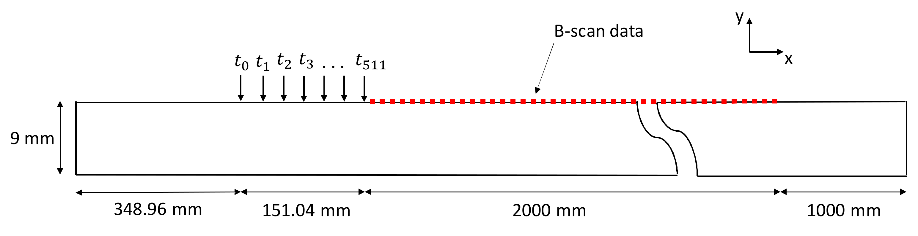
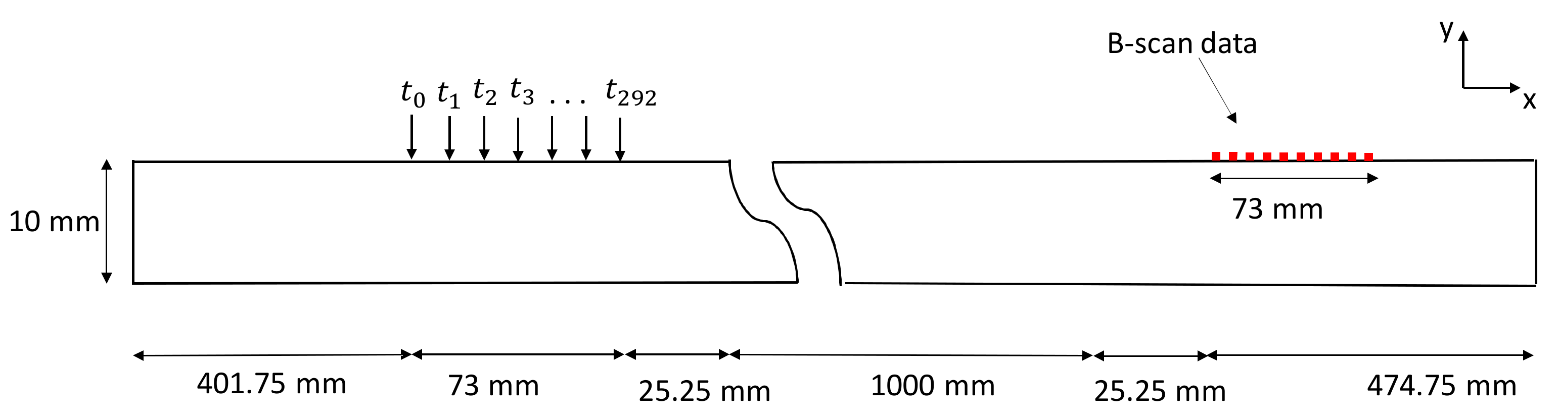
2. Object under Investigation

In this paper, we focus on a 9 mm thickness SteelAlloy1020 plate that mimics unrolled pipe with an outer diameter of 636.6 mm and a circumference of 2 m. The results presented by other authors suggest that Rayleigh–Lame dispersion equations for plates can be used as approximation to obtain dispersion relations in the circumferential direction of the thin cylindrical shell [19,32,33]. This is valid for thin wall pipes, where the ratio between inner (r) and outer (R) radius is r/R > 0.95. Other papers demonstrated that dispersion curves of plates are similar to hollow cylinders for pipe thickness (h) of radius (R) ratios less than 20% [34]. In this paper, we consider cases where r/R > 0.97, while h/R∼3%. Hence the large radius thin-walled pipe can be considered similar to a plate, while the effect of curvature can be most noticeable at low frequencies only. During all calculations, the material properties of SteelAlloy1020 were considered as follows: density 7850 kg/m3, Young’s modulus 207 GPa, and Poisson’s ratio 0.3. Further details concerning the dimensions of the structure and arrangement of the probes are presented in the following chapters next to the description of the finite element models and experimental set-ups.

3. Selection of Appropriate Mode for Assessment of Pipe Corrosion

Selection of the appropriate mode for inspection is one of the key aspects in the success of corrosion level assessment. The mode selection criteria should consider following aspects: mode excitability and receptibility, leakage losses, attenuation, dispersion, and velocity. Each and every aspect of mode selection is discussed further in the subsequent sections.

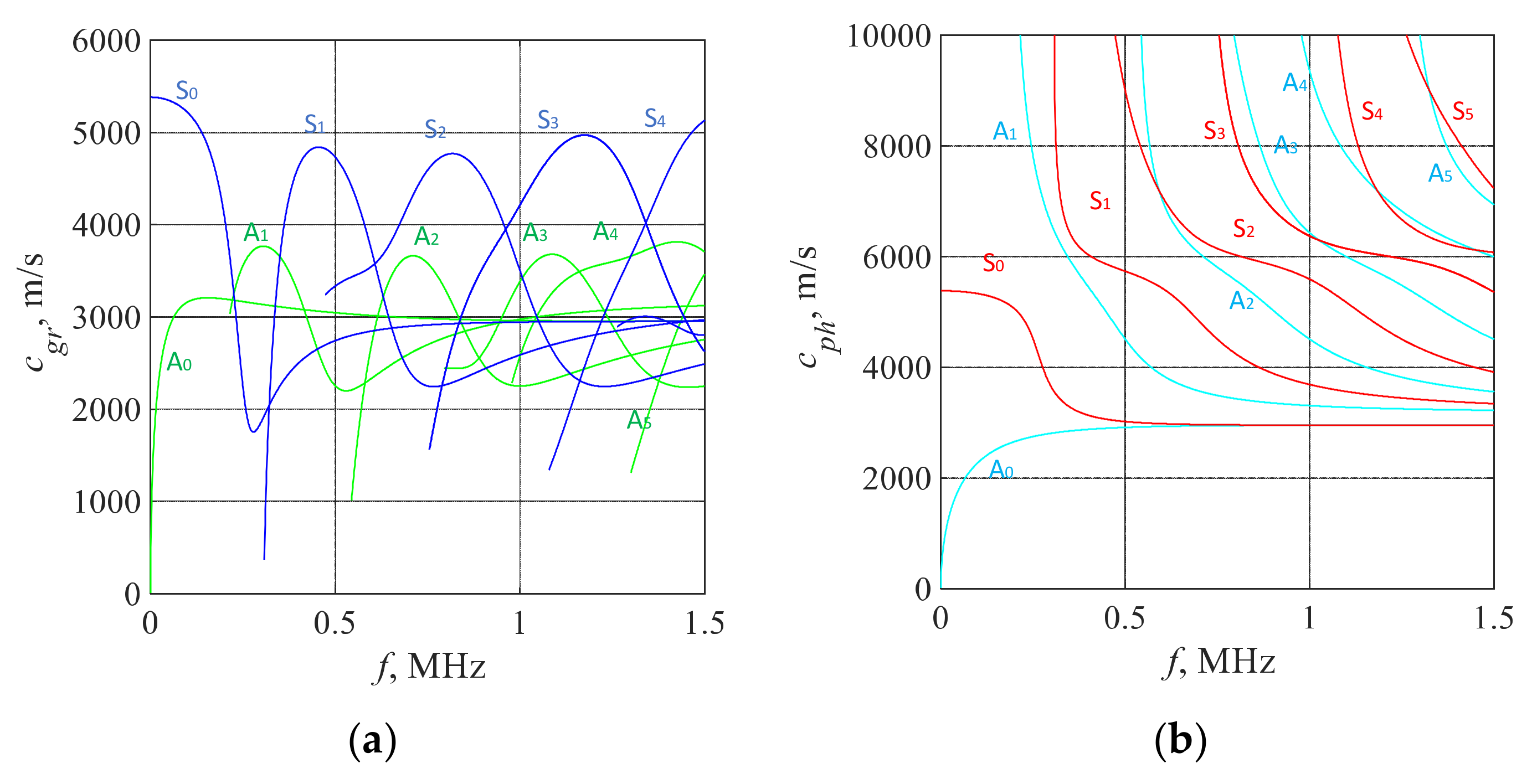
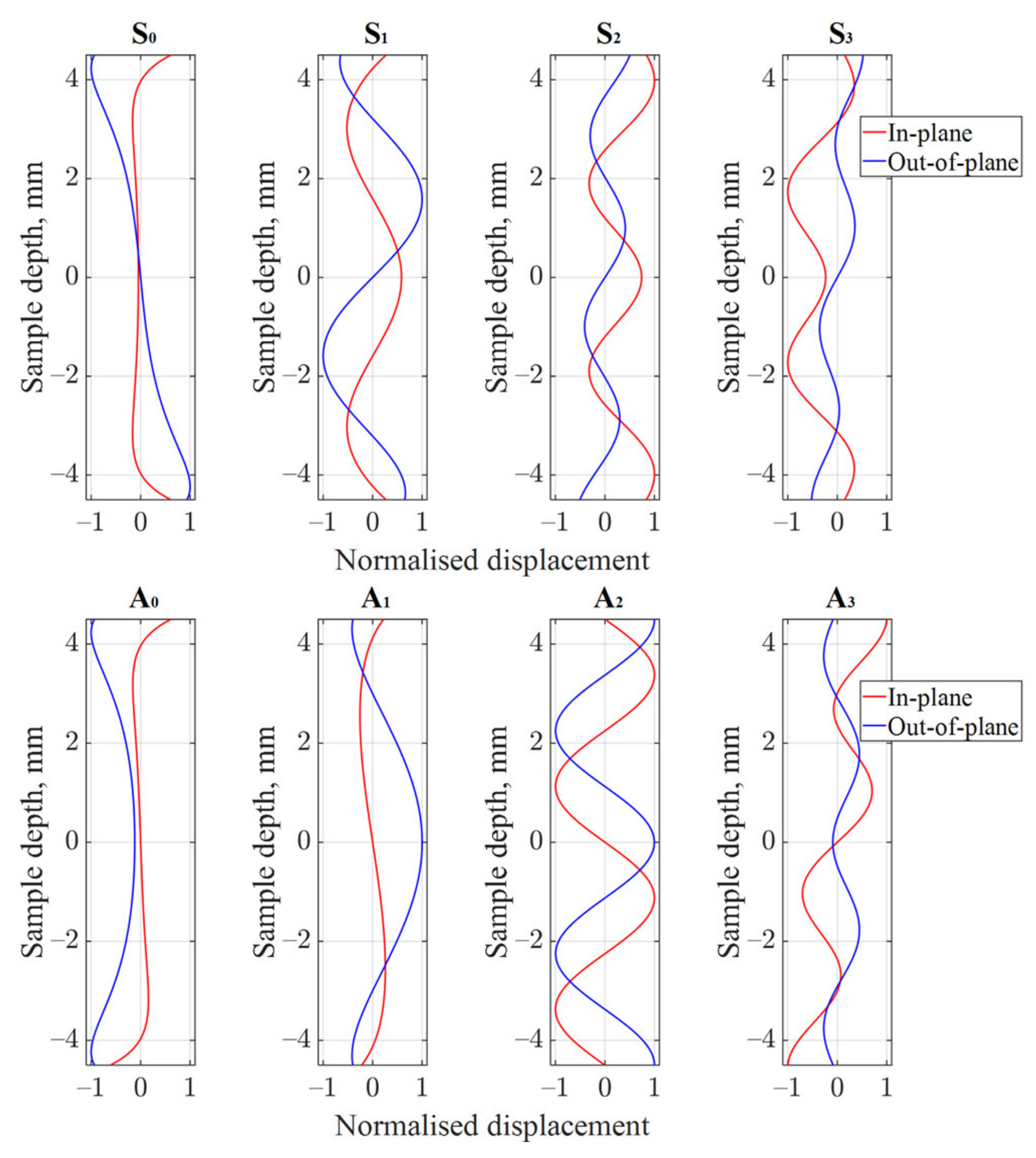
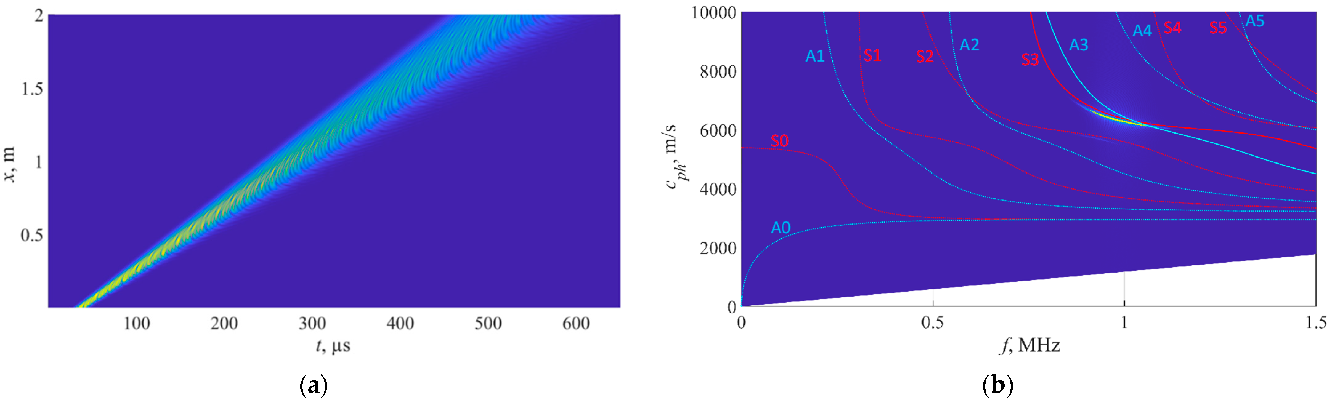
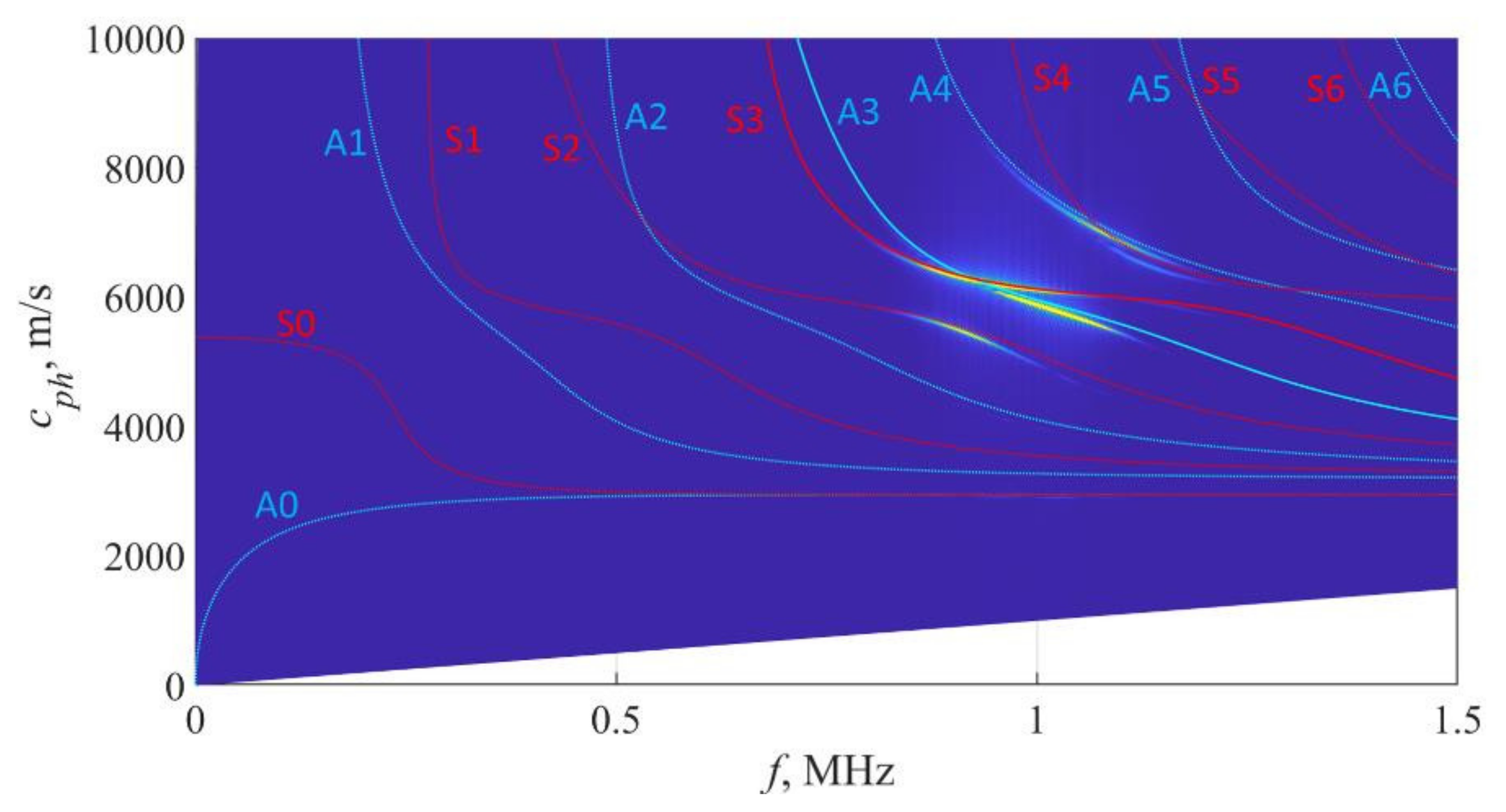
3.1. Dispersion Curves of the Considered Structure

At first stage of the investigations, semi-analytical finite element technique (SAFE) was used to calculate existing dispersion curves, particle displacements, and leakage losses on the unrolled SteelAlloy1020 pipe [35]. The correctness of such approach was stated by other authors [33,34] as it was mentioned above; however, we carried out additional verification by modelling using the FE method, and the validity of plate approximation will be demonstrated later in this chapter, providing a comparison of simulation results between pipes and plates.
In this investigation, dispersion curves were calculated using a 1D plate model and dividing the cross section of the 9 mm plate into 20 discrete elements each with a size of 0.45 mm. Each element was composed of three nodes. Such fine mesh size was deliberately selected as sufficient for the analysis of the displacement profiles of the propagating modes which will be presented later in this chapter [36]. The material properties were used as described in previous chapter. The calculated dispersion characteristics are presented in Figure 1. The dispersion characteristics presented below are considered for the structures exposed to air. The propagation of the modes in pipes filled with water are in some sense different, as the interface between the pipe and water is no longer traction-free. In such case, due to energy leakage to the surrounding media, an interface quasi-Scholte wave starts to propagate in the solid–liquid boundary [37]. This mode has negligible attenuation, short wavelength, and potentially increased sensitivity to small defects. However, at sufficiently high frequencies, it is known to have dominant in-plane displacements in liquid media and thus can no longer be detected from surface of solid structure [38]. The dispersion curves presented in this paper does not consider quasi-Scholte waves as the main purpose of the paper is to explore high order symmetric modes at frequencies, where the quasi-Scholte waves are no longer detectable and possess late arrival time to the sensor.
From the results it can be observed that six asymmetrical and six symmetrical modes exist at frequencies up to 1.5 MHz. Symmetric modes have higher group velocities that peak at certain frequencies, for example, S1 mode at 455 kHz, S2—at 817 kHz and S3—at 1.173 MHz (see Figure 1a). Each peak in group velocity of symmetrical modes corresponds to low-dispersion zone on phase velocity dispersion curves (see Figure 1b). It is preferable to use the mode with fastest group velocity (Figure 1a) as such mode will arrive to the receiver first, simplifying the signal analysis. In this sense the most promising are frequency ranges where group velocities of symmetric modes peaks. However, it is known that at such frequencies the out of plane displacements of particular modes are usually poor, making them difficult to excite and receive using longitudinal ultrasonic transducers [39]. Moreover, in order to preserve the sensitivity to a change in pipe wall thickness that will result in measurable change in group velocity, the excitation frequency should be situated at sloped part of group velocity curve where excited modes are dispersive. As a result, the excitation should be considered at slightly other frequencies (above or below the peak frequency) avoiding that particular zero displacement zone, but still keeping at the dominant group velocity range.
It is necessary to take into account that only the modes that possess a sufficient out-of-plane component in a particular frequency range can be excited using conventional longitudinal wave ultrasonic transducers, which are sensitive to out-of-plane wave motion. On the other hand, the modes which possess strong out-of-plane component will be strongly attenuated due to leakage losses as most of the pipelines are filled with various substances [40]. Therefore, from that point of view, it is necessary to select an optimal mode and corresponding frequency ranges where out-of-plane displacement is sufficient for generation and reception, but on the other hand, it must be sufficiently low in order to have reasonable leakage losses and propagation distance that can be suppressed by conventional ultrasonic amplifiers.
Following the observations presented above, the S3 mode has highest group velocity at frequency band between 0.9 MHz and 1.35 MHz. In such case, the S3 mode is expected to arrive first compared to other modes. At frequencies below 1 MHz, S3 mode has quite dispersive behavior, and hence, it is expected to have high sensitivity to the change in wall thickness of the pipe at a cost of resolution to small defects.
Further parameters that can limit inspection using S3 mode are the leakage losses, attenuation, excitability, and receptibility, which are further explored in subsequent section. All these parameters are related to distribution of particle displacements on the surface of the plate. It the next chapter, the advantages of using S3 mode over neighboring modes such as S1 and S2 will be shown.

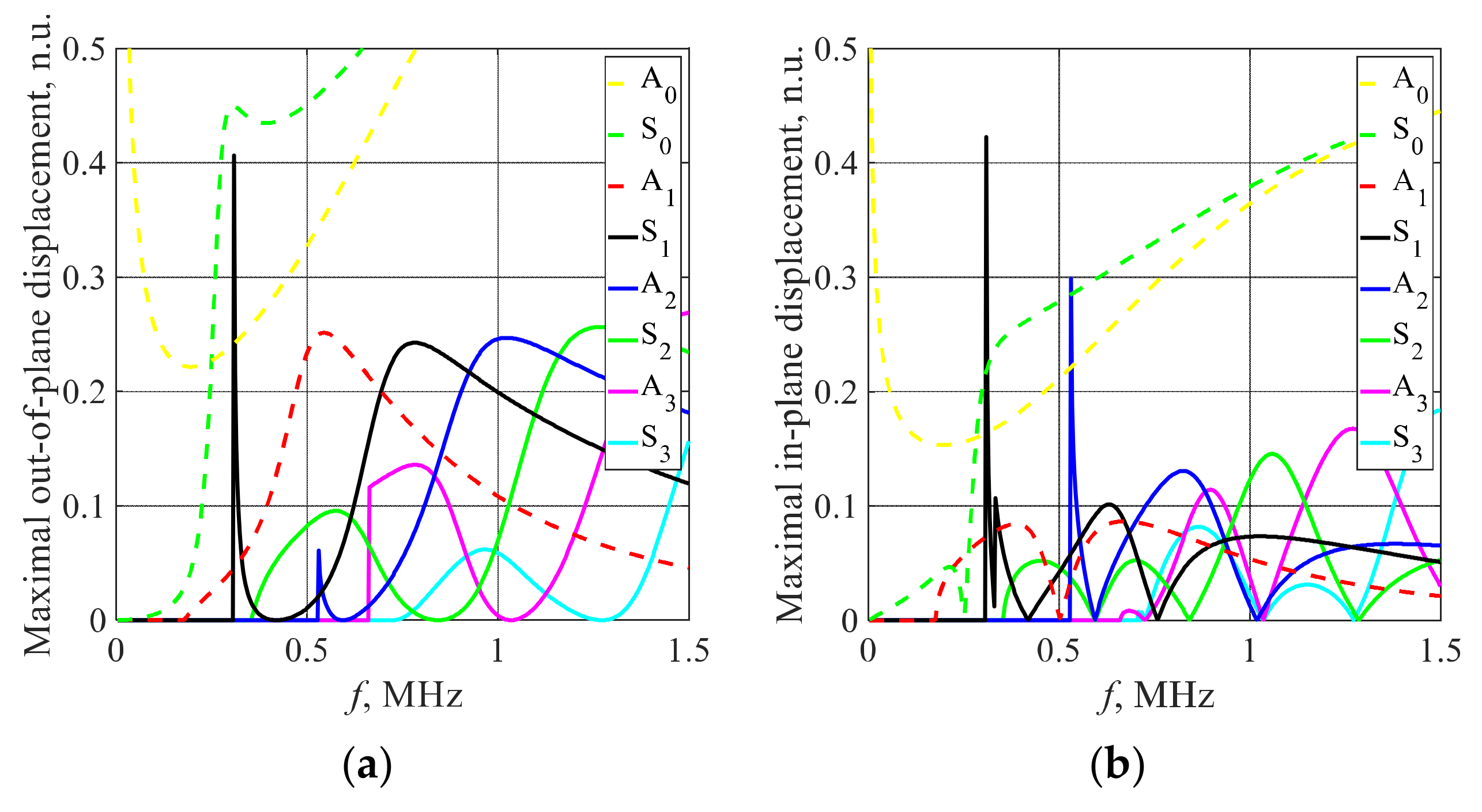
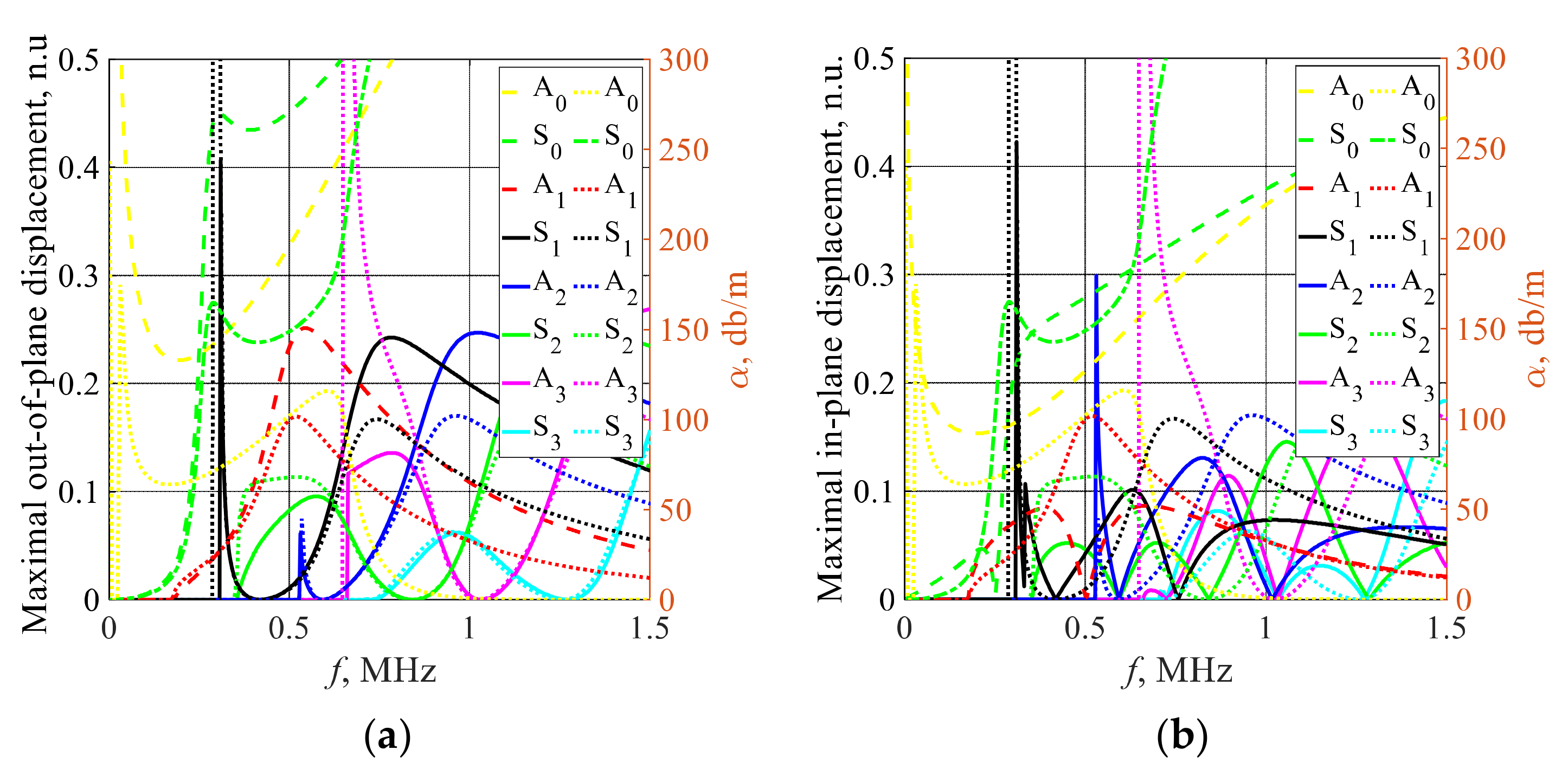
3.2. Leakage Losses and Mode Displacements

Particle velocity and displacement distribution on the surface of the pipe determine the excitability and detectability of the mode and its energy losses to the surrounding media. Conventional longitudinal wave transducers or phased arrays vibrate at a resonant frequency that corresponds to the motion in thickness direction of piezo ceramics. The in-plane displacements cannot be detected by such transducers if these are attached through coupling liquid perpendicularly to the direction of in plane motion. As a result, such probes can excite and receive modes that have a sufficient out-of-plane component. Symmetric modes usually possess quite minor out-of-plane displacements, and thus, only those symmetric modes that have sufficient out-of-plane displacements can be excited with conventional longitudinal wave probes. On the other hand, such probes are effective, generating asymmetric modes and possessing significant out-of-plane displacements. Hence, it can be expected that while trying to excite symmetric modes using the conventional longitudinal wave transducers, undesired asymmetrical modes will be generated also within the selected frequency band. The out-of-plane and in-plane distributions of mode amplitudes at the surface of the steel alloy were calculated using the SAFE method and the same material properties as described in the previous section. The results are presented in Figure 2.
The out of plane component calculations on the surface of steel alloy plate suggest that the S3 mode has quite sufficient out of plane components in the frequency band around 1 MHz to be generated and detected with conventional phased arrays. It can be observed that at these frequencies, other modes such as A1, S1, or A2 will be generated more effectively. From the out-of-plane displacement curves, it can be observed that the S2 mode can be excited starting at around 1 MHz. At this frequency, it has similar out-of-plane components to the S3 mode; however, the displacements rise significantly for S2 mode above 1 MHz.
The out-of-plane component of each specific mode is correlated with the leakage losses. The comparison between the amplitude distribution on the surface with leakage losses and the water loading is presented in Figure 3. As it can be observed, in Figure 3a, the displacement of normal components is strongly correlated with leakage losses, as expected, and less correlated to in-plane displacements as seen in Figure 3b. The leakage losses of the S3 mode at 1 MHz is approximately 34 dB/m, and hence, the S3 mode can be expected to be used at distances of up to 1.5–2 m, which is sufficient for screening of pipes at their cross section with outer diameters up to 640 mm. At such propagation distance, the total losses due to leakage are expected to be in the range 51 dB to 68 dB, which can be compensated by conventional ultrasonic amplifiers. It can be noted that other co-existing modes such as A1, S1, or A2 have either similar (in case of A1 mode) or significantly higher losses (in case of S1 and A2). The losses of S2 mode are similar to S3 at 1 MHz but are much more significant above this frequency.
While the surface displacements show the excitability and leakage of the guided wave modes, the distribution over the thickness of plate determines which defects can be detected. To explore this in more detail, the displacement distribution in the cross section of the plate has been calculated for S3 mode. The results are presented in Figure 4. It can be observed that out-of-plane displacements of S3 mode exist at around 1 MHz frequency only. The out-of-plane displacements are zero at certain depths that correspond to middle thickness and depths of 1.5 mm and 7.5 mm according to the top surface.
To explore the difference between the displacement distribution of the S3 mode and other symmetrical and asymmetrical modes, the normalized displacement distributions of A0-A3 and S0-S3 modes were estimated at 1 MHz and presented in Figure 5. It can be observed in thickness cross-section of displacements that the particle displacement distribution of the S3 mode varies inside the plate but also has sufficient particle displacement on the plate surface. The distribution of the waves across the thickness of the plate is not uniform and should be taken into account when the sensitivity to the different types of defects is analyzed. The results suggest that out-of-plane displacements of the S3 mode peak at the surface of the plate and at depths corresponding to 1 mm and −1 mm with respect to middle thickness of the plate. All symmetrical modes in contrast to asymmetrical ones possess out of plane displacements close to zero at middle thickness. The S2 mode has a strong in-plane component on the surface of the plate and relatively small leakage losses making it suitable for shallow defect detection. On the other hand, the group velocity of S2 is quite low at 1 MHz which will complicate the analysis of arriving signals, while above 1 MHz, the leakage losses of this mode become unacceptable. In contrast, asymmetrical modes A1 and A2 have quite strong middle thickness out-of-plane displacements, but displacements at surface of the sample are quite low for A1 and A3 modes. The A2 mode could be considered as good candidate for corrosion detection; however, essential attenuation limits its applicability.
The results presented above suggest that S3 mode at 1 MHz could be used for corrosion assessment as it has high group velocity, out-of-plane displacements, and acceptable leakage losses for inspections up to 2 m. In subsequent sections, the excitation of the S3 mode will be further explored using finite element model and experiments.

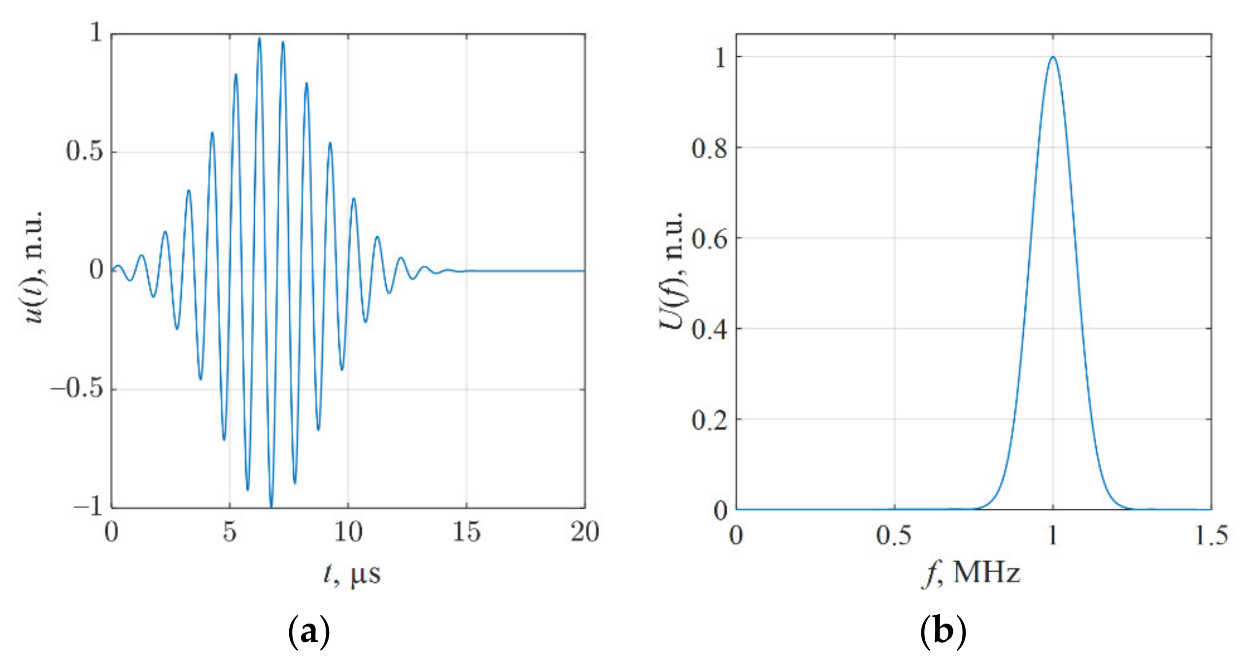
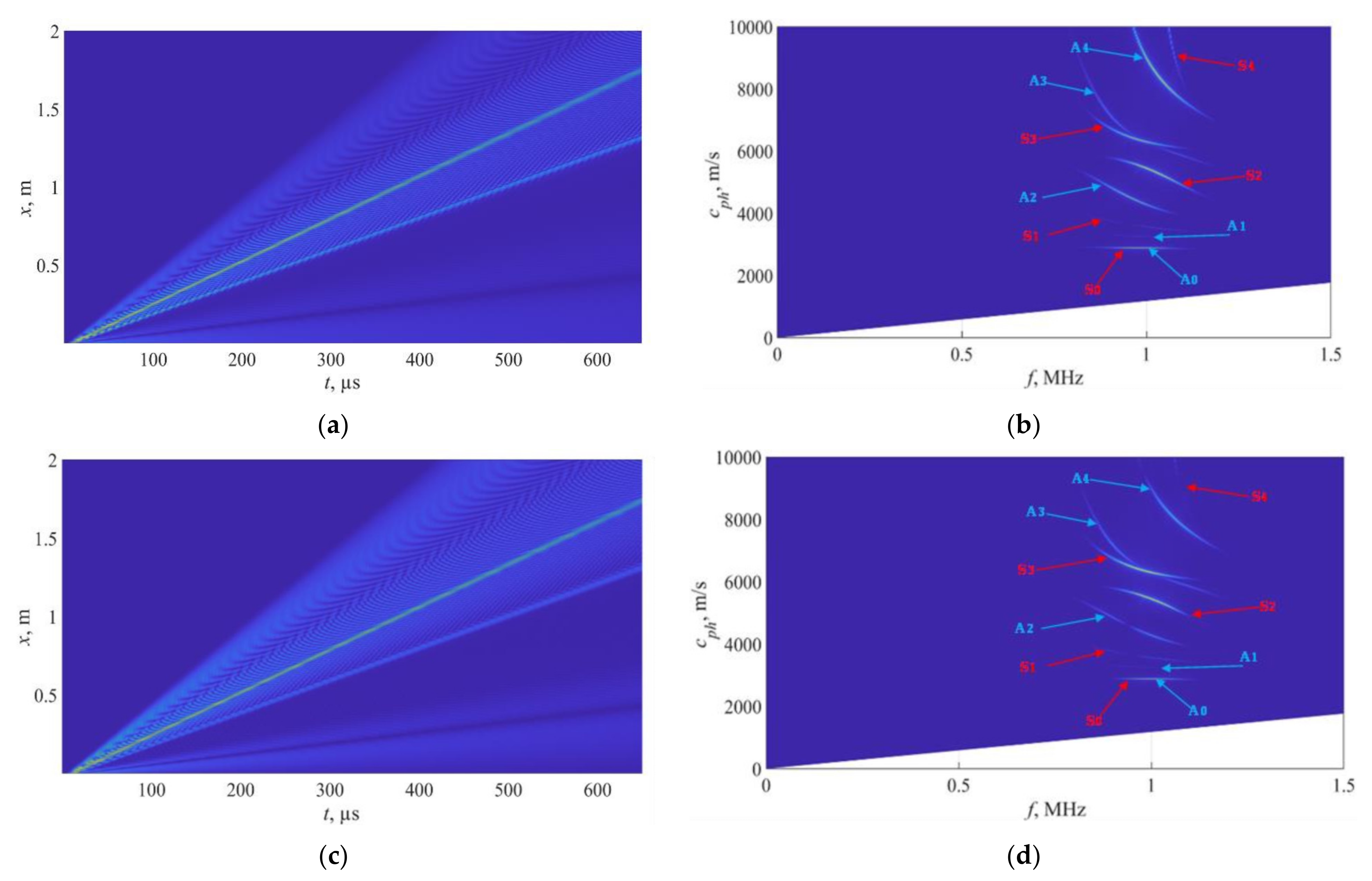
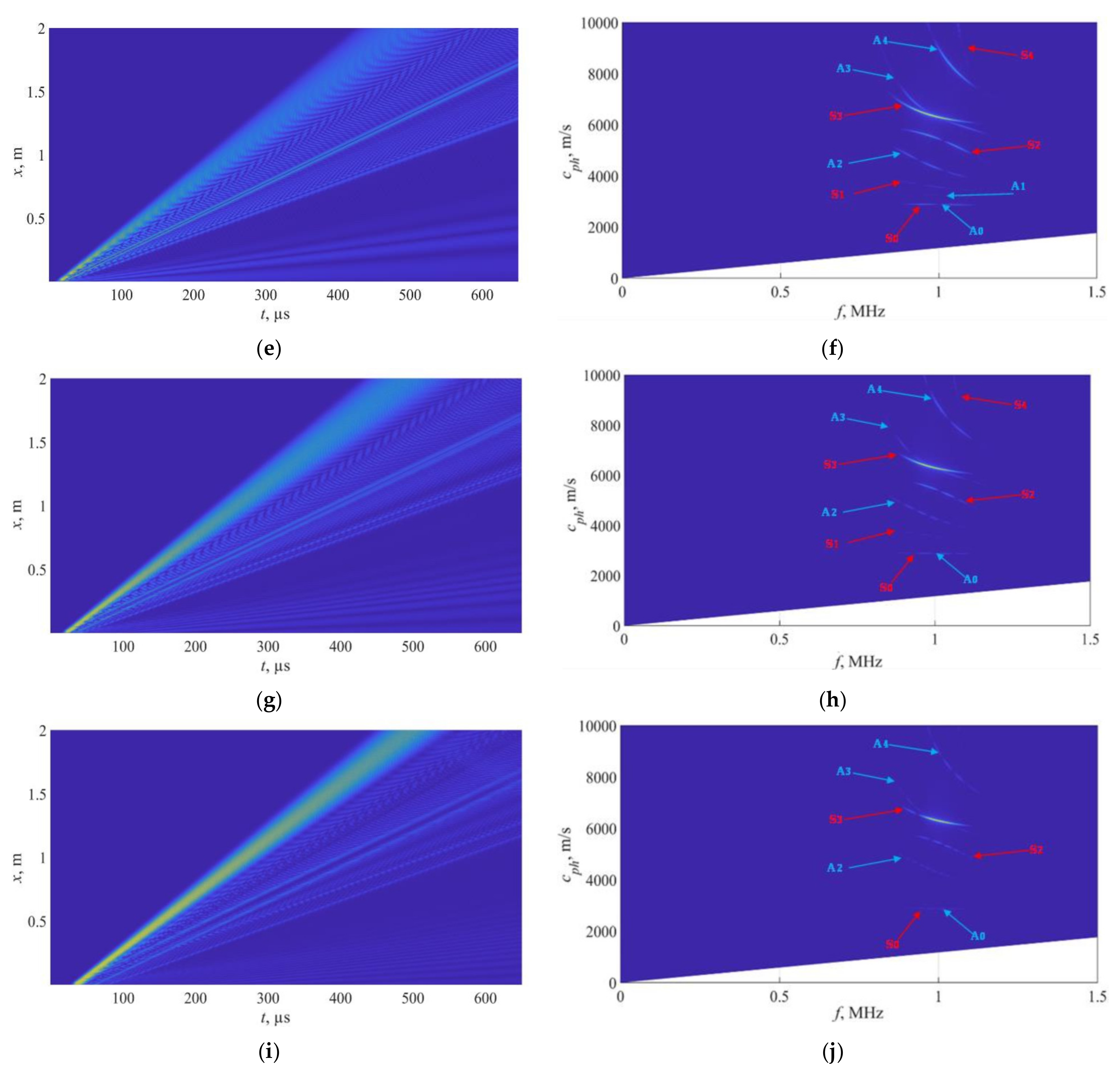
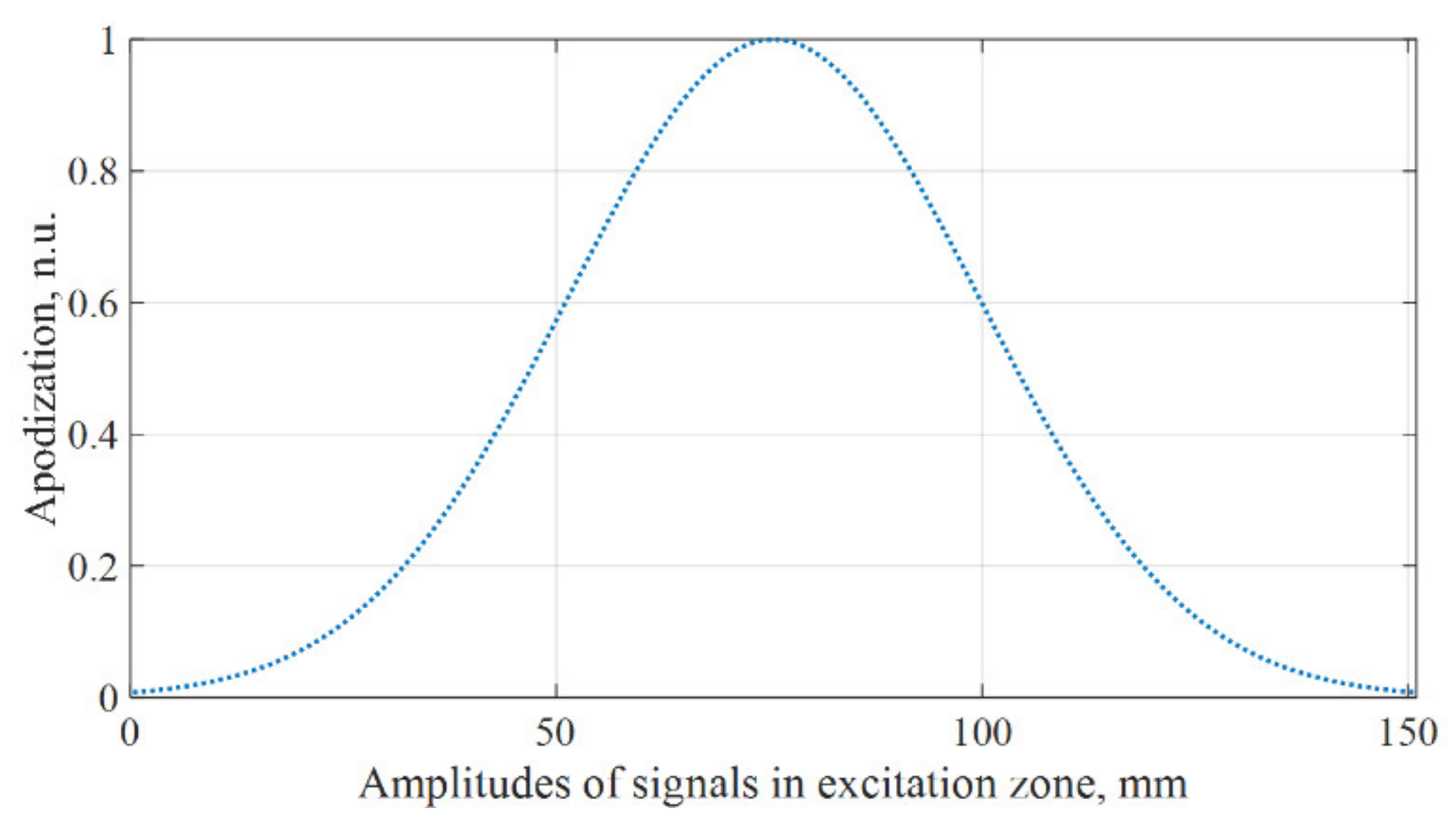
4. The Model for Analysis of S3 Mode Excitation and Propagation

To verify the assumptions made on the previous section, 2D finite element simulations were carried out. The models aimed at investigating excitability of S3 mode and capabilities to avoid generation of undesired co-existing modes while using conventional ultrasonic phased arrays. The geometry of the investigated structure was a rectangle with wave propagating in the direction of longest side along x axis. To avoid interfering reflections from edges of the plate, the length of the model increased to 3.5 m, leaving the monitored segment equal to 2 m as shown in Figure 6. Thus, the overall dimensions of the model were 9 mm × 3.5 m. In this case, we avoided using absorbing boundaries, as in some cases they still can produce weak reflections [41]. To confirm the correctness of the pipe approximation, FE models at particular cases will be generated for pipes as well.
2D linear plane strain finite element model was implemented using Abaqus explicit solver (Dassault Systèmes, Vélizy-Villacoublay, France), assuming that the object is infinite in the z direction. CPE4R four node plane strain elements with reduced integration were chosen for the regular mesh model. The edge length of an element was set to 0.295 mm, which is λ/10 of the slowest mode in the considered frequency band. The integration step in the time domain was set to 0.03 µs, which is 1/33 of the period at 1 MHz central frequency. Both mesh size and integration step met the accuracy requirements of FE structural mechanics problems [36]. The propagating wave in x direction was excited by applying normal to surface force to specific number of nodes on the surface of plate starting at 32 nodes and ending with 512 nodes. This approach has been selected in order to facilitate the phased array excitation with varying aperture as it was shown that the size of array active area determines the bandwidth of excited modes along the phase velocity axis [36]. The example of 1 MHz 10 period Gaussian tone-burst excitation signal that was used throughout the simulations is presented in Figure 7. The variable monitored in this study was an in-plane (x) and out-of-plane (y) component of particle velocity at element nodes located on top surface at distances from 500 mm to 2500 mm from the origin as shown in Figure 6.

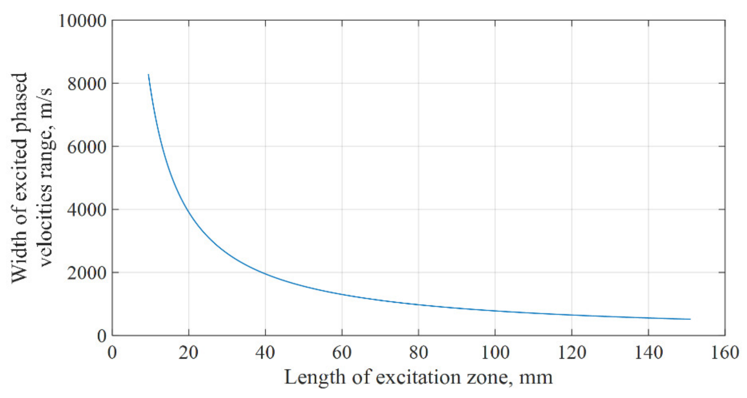
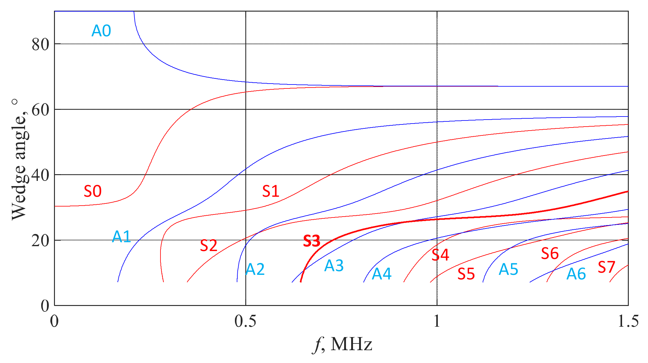
Selective Excitation of S3 Mode

As the guided waves possess many modes in the particular frequency bandwidth, the selective generation should be adjusted both in frequency and phased velocity domain. The frequency bandwidth is determined by the characteristics of ultrasonic transducer and parameters of excitation signal. More complicated is the optimization according to the phase velocity or, in other words, the spatial frequency domain. Unidirectional selective guided wave excitation minimizing other modes at the same time can be implemented by simulating the performance of the corresponding angled probe. As it was shown by other authors, angled plane wave front can be obtained with a phased array where the angle of the wavefront or delay time of array channels determines the specific phased velocity of the wave. Delay times (focal laws) for excitation of mode with particular phase velocity can be calculated using the following equation [35,42]:
t i = p · i 1 c ph ,
where t i is the delay for each element, i is the array element number, p is the pitch, and c ph is the targeted phase velocity.
While the spectrum of the excitation signal determines the limits of the frequency band in which the guided waves are generated, the aperture of the transducer determines the ranges along the phase velocity axis.
In the case of rectangular harmonic burst, the frequency bandwidth of the main lobe of the spectrum can be estimated as 2 t B , where t B is the duration of the burst. Therefore, in order to have a frequency bandwidth of around 0.2 MHz, the duration of the burst should be 10 μs. In case of a 1 MHz excitation frequency, it will correspond to 10 periods burst. In a similar way, it can be shown that the phase velocity bandwidth of generated modes can be determined according to:
Δ c 2 · c 0 2 L ex · f 0 ,
where Lex is the length of excitation zone, f0 is the central frequency, and c0 is the velocity at the central frequency. The phase velocity of S3 mode at 1 MHz is 6250 m/s according to the estimations presented in previous section. Then, the phase velocity bandwidth Δc for this mode, estimated according to Equation (2), will look like the one presented in Figure 8.
In order to verify this assumption, excitation of S3 mode was investigated using fixed delay law, corresponding to phase velocity 6250 m/s, but at the same time, changing the length of excitation zone from 9.44 mm to 151.04 mm. In such case, the phase velocity bandwidth varies from 8300 m/s to 500 m/s, which is expected to limit number of generated modes. Meanwhile the frequency bandwidth remained the same in all cases—0.2 MHz at –6 dB level. In each of the models, the B-scan data of the out-of-plane component on the surface of plate along the x direction was collected. To illustrate the propagating modes, 2D Fourier transform was used to transfer data from the time–distance to the phase velocity–frequency domain [43,44]. The obtained results are presented in Figure 9. It can be observed that in case of small apertures (9.44 mm and 18.88 mm) all modes are excited in the frequency band of input signal, showing wide phase velocity ranges in Figure 9b,d. The phase velocity range is effectively reduced using a 75.52 mm excitation zone Figure 9h. Further increase of the aperture provides even better mode isolation. In reality, the aperture of the array cannot be unlimited, meaning that other undesired modes are likely to be excited, however, with essentially smaller amplitudes. For example, even in the case of a 151 mm aperture, patterns of S3, S2, S0, A4, A3, A2, and A0 modes can be also observed in Figure 9i,j.
This can be explained by the fact that the rectangular distribution of amplitudes in the excitation zone will lead to the appearance of relatively high side lobes in the spatial spectrum. The amplitude of these side lobes can be reduced by smoothing the excitation amplitudes at the edges of excitation zone using apodization. An apodization function (also called a tapering function or window function) is a function used to smoothly bring the amplitudes of the signal down to zero at the edges of the excitation zone. The apodization law is illustrated in Figure 10. Such excitation scenario was implemented for the case of 151 mm excitation zone only to elucidate the improvement in suppression of co-existing modes. The results presented in Figure 11a,b show that a very weak pattern of A3 and S2 modes still can be observed, while other modes like S0, A4, A2, and A0 vanished. In order to demonstrate the validity of the unrolled pipe approximation, the same excitation with apodization was implemented for a 2D pipe structure with circumference of 2 m. The results presented in Figure 11c,d found to be similar to the ones obtained on a plate. Similar patterns of A3 and S2 modes as well as wave crossing points can be observed, suggesting the validity of the plate approximation.
In order to suppress the existing A3 asymmetric mode, excitation from both sides of the plate with the same apodization was implemented instead of increasing excitation zone. The results of simulation can be seen in Figure 12. It can be observed, that in this case, a pure S3 mode is propagating in the structure. While such two-sided excitation approach is unpractical, it has big advantage in the modelling as it enables to analyze separately interaction of S3 mode with defects. In this way, only S3 mode can be explored avoiding the presence of other modes that may lead to contradicting results.
Taken together, these results demonstrate, that suppression of co-existing modes can be achieved by implementing delays to subsequent nodes, apodization, and two-sided excitation. In the next section, the excitation of S3 and co-existing modes are explored with experiments.

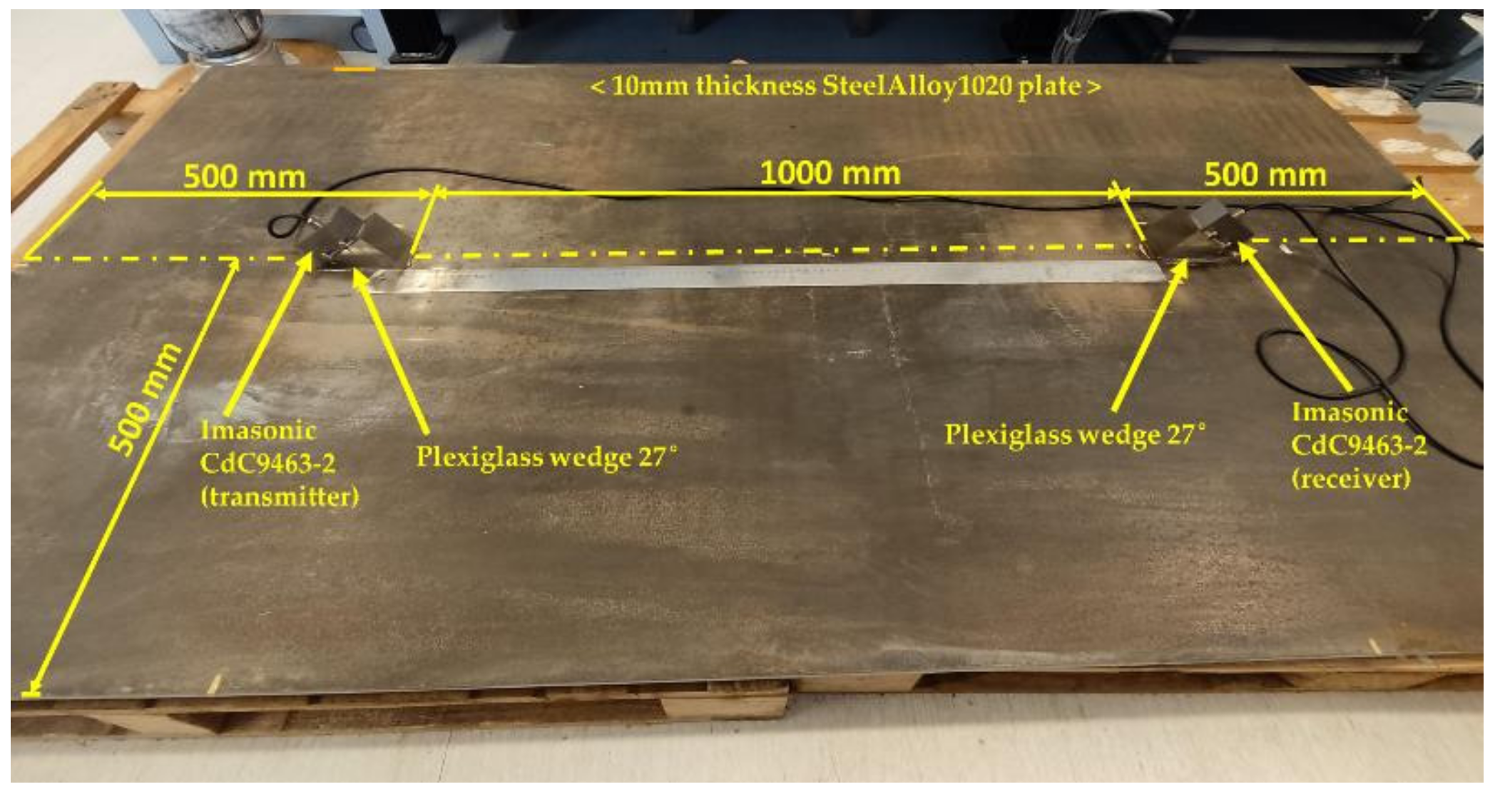
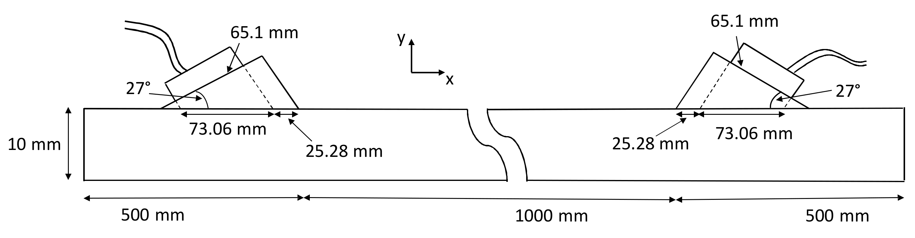
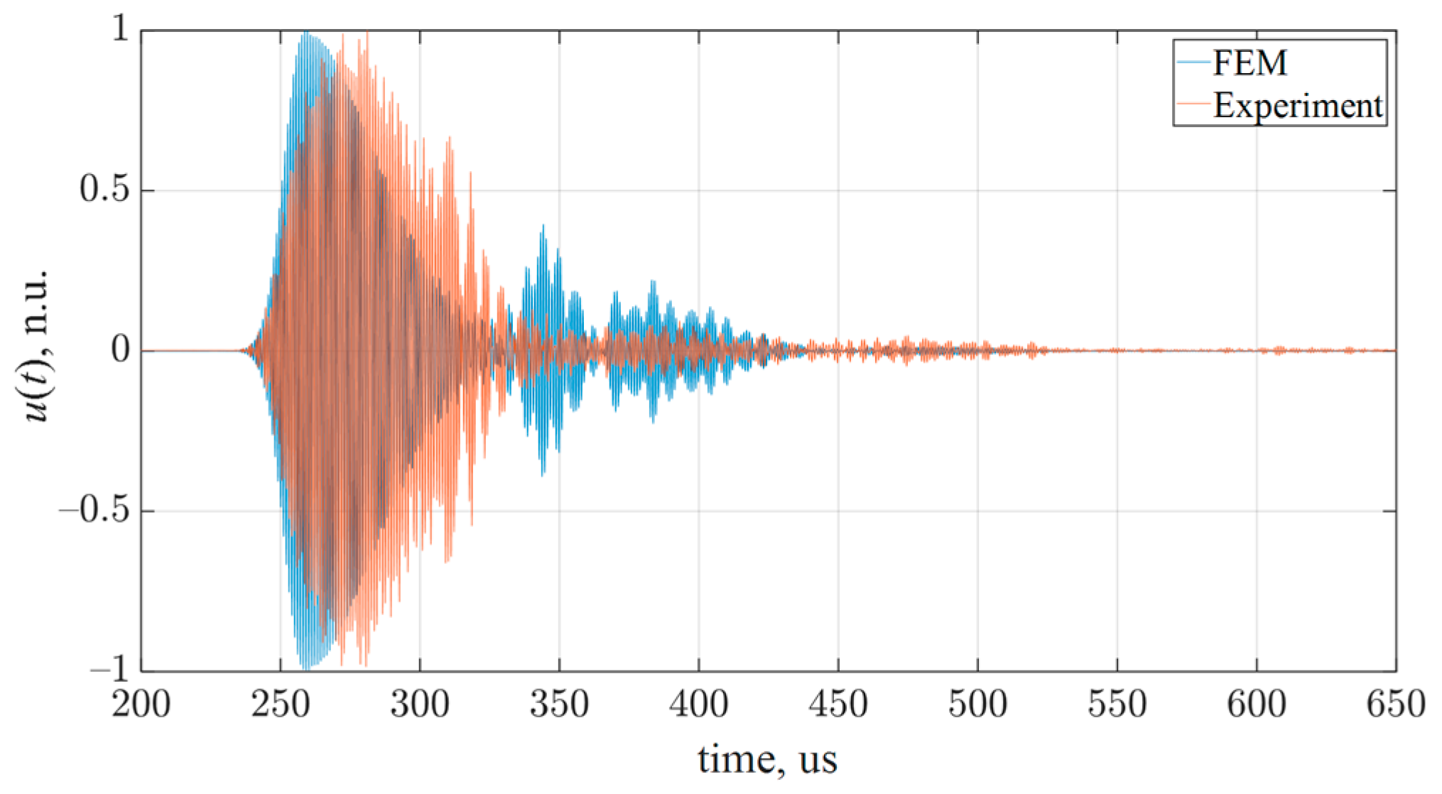
5. Experimental Validation

To verify the simulation results, which demonstrated possibility to excite symmetric S3 mode while suppressing co-existing modes, experiments were carried out. For this purpose, 10 mm thickness SteelAlloy1020 plate with dimensions 1000 mm × 2000 mm was selected. Two 1 MHz 32 element Imasonic CdC9463-2 phased arrays with pitch of 2.05 mm and active aperture of 65.1 mm were arranged in pitch-catch configuration and placed 1000 mm apart. The bandwidth of the selected probe is 57% at –6 dB. To generate and record signals of propagating modes, the multichannel data acquisition system Dasel Sitau (Dasel Sistemas, Madrid, Spain) with 128 parallel channels was used. The view and schematic diagram of experimental arrangement are presented in Figure 13 and Figure 14, respectively.
Throughout the experiments, special 27° plexiglass wedges were manufactured and used as the interface between the array and the sample. Such specific wedge angle was selected according to the excitation angle curves, which were calculated for 10 mm thickness steel plate and are presented in Figure 15. According to the results, presented in Figure 15, the excitation angle for S3 mode at 1 MHz is 26.35° where phase velocity is equal to 6127 m/s. In order to set proper incidence angle, the wavefront of the plane wave generated by phased array was slightly steered by 0.65° changing delay laws t s t i of each array element in order to achieve exactly 26.35° incidence:
t s t i = p · i 1 sin α s t C L ,
where t s t i is the steering delay of each element, p is the element pitch, i is the element number, C L is the longitudinal velocity in plexiglass prism, α s t is the steering angle. At 27° angle, a projection of the wave-front on the surface of the steel plate is equal to 73.06 mm, and this is considered as array aperture throughout this experiment.
Since the experiment was carried out on a 10 mm plate while the simulations presented earlier were carried out on 9 mm thickness sample, a new FE model was conducted here which mimics the conditions of the experiment. In this model, a zone equal to 73 mm was excited using normal to surface force, and particle velocity at the nodal points located 1123.5 mm away from the transmission zone were collected. Such distance takes into account the dimensions of the Plexiglas wedges and 1000 mm distance between them corresponding to the experiment. The schematic diagram of FE model is presented in Figure 16.
During experiments, the signals were recorded separately by each element. Both, experimental and modelled signals then were integrated, considering the phasing angle and in such a way simulating performance of the phased array. Integration was implemented according to the following equation:
u t = i = 1 K u i t t st , i ,
where u i t is the signals measured by i th phased array element; K is the total number of elements in phased array; t s t , i is the phasing delay calculated according to Equation (3). The signals obtained from the FE model and experiment are presented in Figure 17.
Simulation and experimental results show good agreement for S3 wave mode. A significant difference can be observed at the trail of the signals, which is due to the appearance of slower modes. From the 2D FFT data of FE model (Figure 18), it can be observed that weak patters of S2, A3, A4, and S4 modes are still visible. However, as the S3 mode exhibits high group velocity, it will not overlap with co-existing modes at sufficient distances. The generation of parasitic A4, S4, and S2 modes can be suppressed by limiting the frequency bandwidth of the probe while increasing the cycle count of the excitation signal. A4, S4, and S2 mode generation is also determined by limited size of the active aperture.

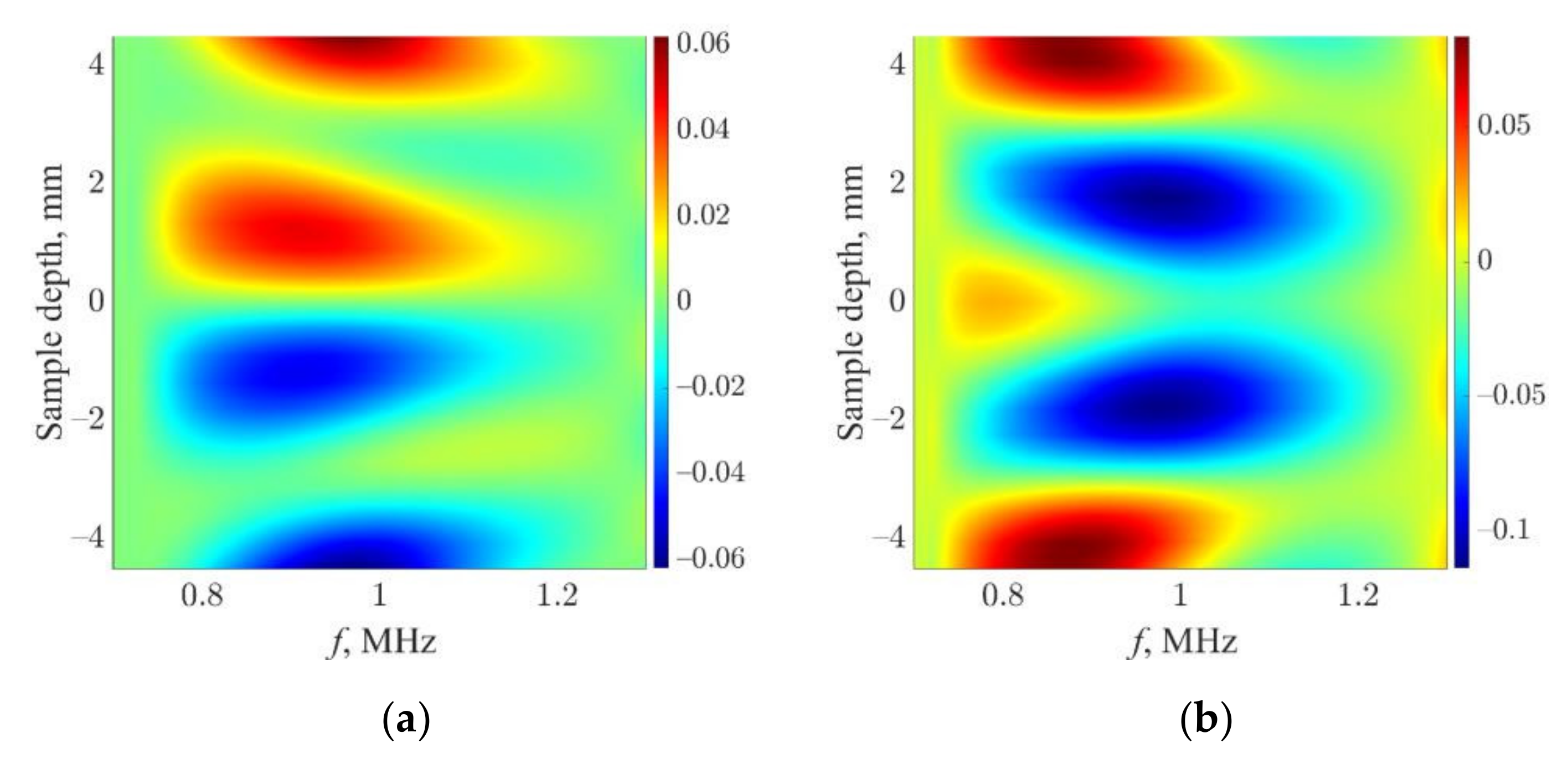
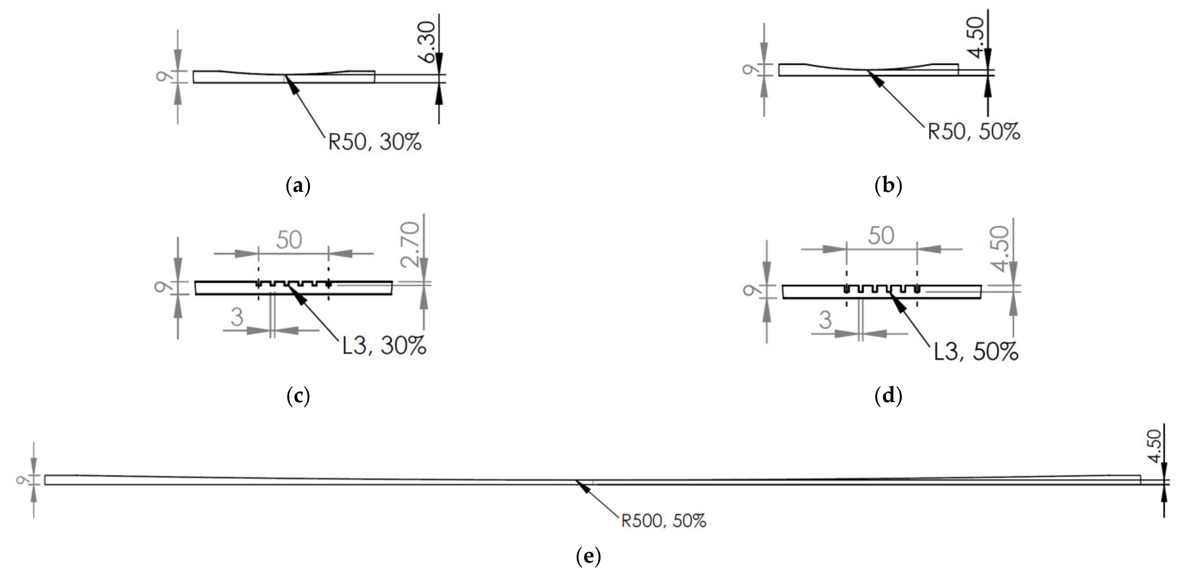
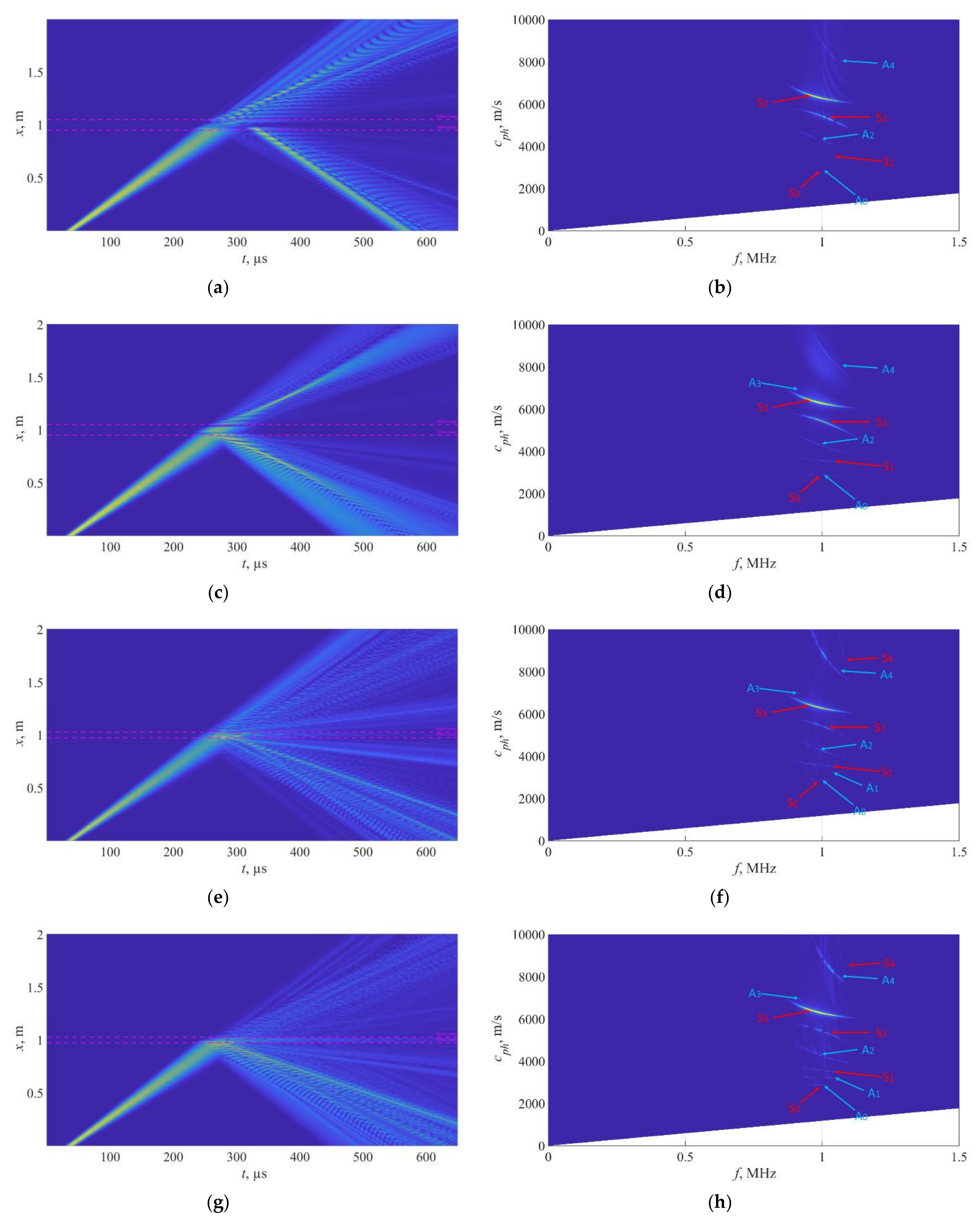
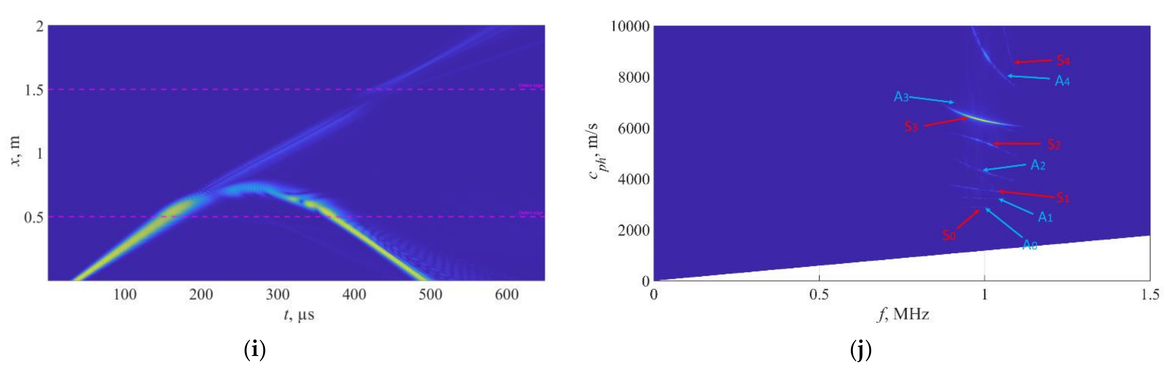
6. Interaction of S3 Mode with Corrosion Equivalent Defects

Having outlined the conceptual principles of excitation of isolated S3 mode, in this chapter, mode response to synthetic corrosion-like defects is investigated. 2D FE models with different extent of wall thickness loss were used for a virtual experiment. While the unrolled pipe approach has been validated earlier, synthetic models represented a plate scenario. In total, three different types of defects that mimic wall thickness loss due to corrosion were considered, namely, localized, pitting, and uniform. Localized corrosion was simulated as cylindrical cut with radius of 50 mm and depth of 30% and 50% of the initial wall thickness of the model. Pitting defect was considered as a cluster of 3 mm wide rectangular cuts evenly spaced at 50 mm zone. The pitch between the cuts was set to 10 mm, leading to 6 successive defects in the considered area. Two cases of pitting defect were executed, 30% and 50% of the total wall thickness. Finally, the uniform defect was implemented as 1000 mm zone with gradual wall thickness loss, reaching a 50% of the initial wall thickness at 500 mm distance. Cases considered at simulations are illustrated in Figure 19.
The calculations were executed using Abaqus explicit FE solver (Dassault Systèmes, Vélizy-Villacoublay, France), creating a 2D plane strain FE model for each case. The propagation of the S3 mode was simulated in the 2000 mm zone, while the defects were centered at 1000 mm. The uniform mesh size of 0.295 mm was used in the areas outside the defects. In the defect regions, the edges of the model were seeded providing a minimum allowed element size of 0.16 mm. The integration step in the time domain was set to 0.03 µs, which is 1/33 of the period at 1 MHz central frequency. The wave propagating in x direction was excited by applying normal to surface force to a 151.04 mm zone using the symmetrical two-sided excitation and apodization as it was discussed in chapter 4. The S3 mode was excited with a 10 period 1 MHz Gaussian tone-burst excitation signal. The variable monitored in this study was out-of-plane (y) component of particle velocity at nodes located on the outer surface of the plate. Figure 20 shows the obtained Bscans of the out-of-plane component and corresponding 2D FFT images in case of different types of defects.
Various defects show different outcomes of the interaction with S3 mode. For example, localized defects (Figure 20a–d) produce quite strong converted S2 mode, which propagates with lower group velocity and arrives after the direct S3 mode. The presence of S2 mode in case of pitting defects (Figure 20e–h) is no longer that evident. It can be speculated that multiple scattering and mode conversion takes place at each cut of pitting defect providing a diffused ultrasonic signal at the output. A uniform defect (Figure 20i,j) does not show any mode conversion; however, significant delay of the S3 arrival can be expected. The presented results suggest the usefulness of the S3 mode in detecting defects that mimic different types of corrosion. The detailed analysis of the S3 mode response to defects was out of the scope of this paper and remains a subject for the follow-up paper.

7. Conclusions

In this paper, higher order symmetrical modes suitable for corrosion detection were analyzed, employing the dispersion relations, in-plane and out-of-plane distributions, and leakage to surrounding media. It was determined, that S3 mode could be a good candidate for corrosion assessment, as it has sufficiently short wavelength, possess relatively low attenuation and can be excited and received using conventional ultrasonic phased arrays. Finite element simulations demonstrated that it is possible to generate a pure S3 mode, by using phased excitation with a sufficiently large aperture, by decreasing side lobes using apodization towards the edges of excitation zone, and by implementation of two-sided excitation to avoid the presence of asymmetric modes. The model obtained in this study can be used for further analysis of the S3 mode interaction with defects typical to corroded structures.
It was demonstrated through experiments that the S3 mode can be generated in the structure using conventional phased arrays. A good agreement was found between the modelling and the experiments. Despite the experiments demonstrated presence of parasitic modes, the high group velocity of S3 allows to distinguish it from the surrounding signals quite easily at sufficient propagation distances. The findings presented in this paper suggest using a high order symmetric mode for corrosion assessment and demonstrate how different techniques based on phased array or angled excitation could be used in order to excite a selected wave mode into the structure minimizing generation of undesired waves.
Finally, it has been demonstrated that S3 mode is sensitive both to localized and distributed defects that correspond to the corrosion of metallic structures. To date, this mode has been used for such defect detection for the first time and can be used for rapid screening around the circumference of the pipe. The detailed interaction between the S3 mode and defects of various types remains the subject of a follow-up paper.

Author Contributions

Conceptualization, D.C.; methodology, V.S., L.M., R.R., and E.Ž.; software, V.S., and L.M.; validation, D.C., and L.M.; formal analysis, D.C.; investigation, D.C., V.S., and E.Ž.; resources, D.C., V.S., L.M; data curation, R.R.; writing—original draft preparation, D.C.; writing—review and editing, D.C., V.S., L.M., R.R., and E.Ž.; visualization, D.C., V.S.; supervision, V.S. All authors have read and agreed to the published version of the manuscript.

Funding

This research was funded by the Research Foundation of the Research Council of Lithuania under the project POLITE “Assessment of the distributed and concentrated pipeline corrosion by means of ultrasonic testing and machine learning methods”, No. MIP2113.

Institutional Review Board Statement

Not applicable.

Informed Consent Statement

Not applicable.

Data Availability Statement

Not applicable.

Conflicts of Interest

The authors declare no conflict of interest.

References

  1. Wood, M.; Vetere Arellano, A.L.; Wijk, L. Corrosion-Related Accidents in Petroleum Refineries Lessons Learned from Accidents in EU and OECD Countries; Publications Office of the European Union: Luxembourg, 2013. [Google Scholar] [CrossRef]
  2. Koch, G. 1—Cost of corrosion. In Trends in Oil and Gas Corrosion Research and Technologies; El-Sherik, A.M., Ed.; Woodhead Publishing: Boston, MA, USA, 2017; pp. 3–30. [Google Scholar] [CrossRef]
  3. Makhlouf, A.S.H.; Herrera, V.; Muñoz, E. Corrosion and protection of the metallic structures in the petroleum industry due to corrosion and the techniques for protection. In Handbook of Materials Failure Analysis; Makhlouf, A.S.H., Aliofkhazraei, M., Eds.; Butterworth-Heinemann: Oxford, UK, 2018; Chapter 6; pp. 107–122. [Google Scholar] [CrossRef]
  4. Whillock, G.O.H.; Dunnett, B.F. Intergranular Corrosion of Stainless Steels: A Method to Determine the Long-Term Corrosion Rate of Plate Surfaces from Short-Term Coupon Tests. Corrosion 2003, 59, 274–283. [Google Scholar] [CrossRef]
  5. Hou, Y.; Aldrich, C.; Lepkova, K.; Machuca, L.L.; Kinsella, B. Monitoring of Carbon Steel Corrosion by use of Electrochemical Noise and Recurrence Quantification Analysis. Corros. Sci. 2016, 112, 63–72. [Google Scholar] [CrossRef] [Green Version]
  6. Reiber, S.; Ferguson, J.F.; Benjamin, M.M. An Improved Method for Corrosion-Rate Measurement by Weight Loss. J. Am. Water Work. Assoc. 1988, 80, 41–46. [Google Scholar] [CrossRef]
  7. Honarvar, F.; Salehi, F.; Safavi, V.; Mokhtari, A.; Sinclair, A.N. Ultrasonic Monitoring of Erosion/Corrosion Thinning Rates in Industrial Piping Systems. Ultrasonics 2013, 53, 1251–1258. [Google Scholar] [CrossRef] [PubMed]
  8. Zou, F.; Cegla, F.B. On Quantitative Corrosion Rate Monitoring with Ultrasound. J. Electroanal. Chem. 2018, 812, 115–121. [Google Scholar] [CrossRef]
  9. Zou, F.; Cegla, F.B. High Accuracy Ultrasonic Monitoring of Electrochemical Processes. Electrochem. Commun. 2017, 82, 134–138. [Google Scholar] [CrossRef]
  10. Benstock, D.; Cegla, F.; Stone, M. The Influence of Surface Roughness on Ultrasonic Thickness Measurements. J. Acoust. Soc. Am. 2014, 136, 3028–3039. [Google Scholar] [CrossRef] [Green Version]
  11. Gajdacsi, A.; Cegla, F. The Effect of Corrosion Induced Surface Morphology Changes on Ultrasonically Monitored Corrosion Rates. Smart Mater. Struct. 2016, 25, 115010. [Google Scholar] [CrossRef] [Green Version]
  12. Cegla, F.; Gajdacsi, A. Mitigating the Effects of Surface Morphology Changes during Ultrasonic Wall Thickness Monitoring. AIP Conf. Proc. 2016, 1706, 170001. [Google Scholar] [CrossRef] [Green Version]
  13. Rommetveit, T.; Johansen, T.F.; Johnsen, R. A Combined Approach for High-Resolution Corrosion Monitoring and Temperature Compensation using Ultrasound. IEEE Trans. Instrum. Meas. 2010, 59, 2843–2853. [Google Scholar] [CrossRef]
  14. Wong, B.; McCann, J.A. McCann. Failure Detection Methods for Pipeline Networks: From Acoustic Sensing to Cyber-Physical Systems. Sensors 2021, 21, 4959. [Google Scholar] [CrossRef]
  15. Kain, V.; Roychowdhury, S.; Ahmedabadi, P.; Barua, D.K. Flow Accelerated Corrosion: Experience from Examination of Components from Nuclear Power Plants. Eng. Fail. Anal. 2011, 18, 2028–2041. [Google Scholar] [CrossRef]
  16. Catton, P.; Mudge, P.; Balachandran, W. Advances in Defect Characterisation using Long-Range Ultrasonic Testing of Pipes. Insight 2008, 50, 480–484. [Google Scholar] [CrossRef]
  17. Fromme, P. Guided Wave Testing. In Handbook of Advanced Non-Destructive Evaluation; Ida, N., Meyendorf, N., Eds.; Springer: Cham, Switzerland, 2018. [Google Scholar]
  18. Howard, R.; Cegla, F. Detectability of Corrosion Damage with Circumferential Guided Waves in Reflection and Transmission. NDT E Int. 2017, 91, 108–119. [Google Scholar] [CrossRef]
  19. Howard, R.; Cegla, F. On the Probability of Detecting Wall Thinning Defects with Dispersive Circumferential Guided Waves. NDT E Int. 2017, 86, 73–82. [Google Scholar] [CrossRef]
  20. Shivaraj, K.; Balasubramaniam, K.; Krishnamurthy, C.V.; Wadhwan, R. Ultrasonic Circumferential Guided Wave for Pitting-Type Corrosion Imaging at Inaccessible Pipe-Support Locations. J. Press. Vessel Technol. 2008, 130, 215021. [Google Scholar] [CrossRef]
  21. Instanes, G.; Toppe, M.; Lakshminarayan, B.; Nagy, P.B. Corrosion and Erosion Monitoring of Pipes by an Ultrasonic Guided Wave Method. In Advanced Ultrasonic Methods for Material and Structure Inspection; Kundu, T., Ed.; ISTE: London, UK, 2007; pp. 115–157. [Google Scholar] [CrossRef]
  22. Na, W.; Kundu, T. A Combination of PZT and EMAT Transducers for Interface Inspection. J. Acoust. Soc. Am. 2002, 111, 2128–2139. [Google Scholar] [CrossRef]
  23. Ostachowicz, W.; Kudela, P.; Krawczuk, M.; Zak, A. Guided Waves in Structures for SHM: The Time-Domain Spectral Element Method; John Wiley & Sons, Ltd.: New York, NY, USA, 2012. [Google Scholar] [CrossRef]
  24. Liu, S.; Chai, K.; Zhang, C.; Jin, L.; Yang, Q. Electromagnetic Acoustic Detection of Steel Plate Defects Based on High-Energy Pulse Excitation. Appl. Sci. 2020, 10, 5534. [Google Scholar] [CrossRef]
  25. Khalili, P.; Cawley, P. The Choice of Ultrasonic Inspection Method for the Detection of Corrosion at Inaccessible Locations. NDT E Int. 2018, 99, 80–92. [Google Scholar] [CrossRef]
  26. Khalili, P.; Cegla, F. Excitation of Single-Mode Shear-Horizontal Guided Waves and Evaluation of their Sensitivity to very Shallow Crack-Like Defects. IEEE Trans. Ultrason. Ferroelectr. Freq. Control 2021, 68, 818–828. [Google Scholar] [CrossRef]
  27. Khalili, P.; Cawley, P. Excitation of Single-Mode Lamb Waves at High-Frequency-Thickness Products. IEEE Trans. Ultrason. Ferroelectr. Freq. Control 2016, 63, 303–312. [Google Scholar] [CrossRef] [Green Version]
  28. Serey, V.; Quaegebeur, N.; Renier, M.; Micheau, P.; Masson, P.; Castaings, M. Selective Generation of Ultrasonic Guided Waves for Damage Detection in Rectangular Bars. Struct. Health Monit. 2021, 20, 1156–1168. [Google Scholar] [CrossRef]
  29. Park, S.; Joo, Y.; Kim, H.; Kim, S. Selective Generation of Lamb Wave Modes in a Finite-Width Plate by Angle-Beam Excitation Method. Sensors 2020, 20, 3868. [Google Scholar] [CrossRef]
  30. Jankauskas, A.; Mazeika, L. Ultrasonic Guided Wave Propagation through Welded Lap Joints. Metals 2016, 6, 315. [Google Scholar] [CrossRef] [Green Version]
  31. Mažeika, L.; Raišutis, R.; Maciulevičius, A.; Žukauskas, E.; Kažys, R.; Seniūnas, G.; Vladišauskas, A. Comparison of several Techniques of Ultrasonic Lamb Waves Velocities Measurements. Ultragarsas 2009, 64, 11–17. [Google Scholar]
  32. Liu, G.; Qu, J. Guided Circumferential Waves in a Circular Annulus. J. Appl. Mech. 1998, 65, 424–430. [Google Scholar] [CrossRef]
  33. Khajeh, E.; Breon, L.; Rose, J.L. Guided Wave Propagation in Complex Curved Waveguides I: Method Introduction and Verification. arXiv 2012, arXiv:1208.6290. [Google Scholar]
  34. Luo, W.; Zhao, X.; Rose, J.L. A Guided Wave Plate Experiment for a Pipe. J. Press. Vessel Technol. 2005, 127, 345–350. [Google Scholar] [CrossRef]
  35. Veit, G.; Bélanger, P. An Ultrasonic Guided Wave Excitation Method at Constant Phase Velocity using Ultrasonic Phased Array Probes. Ultrasonics 2020, 102, 106039. [Google Scholar] [CrossRef]
  36. Qi, X.; Zhao, X. Guided Wave Propagation in Solid Structures of Arbitrary Cross-section Coupled to Infinite Media. AIP Conf. Proc. 2010, 1211, 1681–1688. [Google Scholar] [CrossRef]
  37. Hu, X.; Ng, C.T.; Kotousov, A. Scattering Characteristics of Quasi-Scholte Waves at Blind Holes in Metallic Plates with One Side Exposed to Water. NDT E Int. 2021, 117, 102379. [Google Scholar] [CrossRef]
  38. Cegla, F.B.; Cawley, P.; Lowe, M.J.S. Material Property Measurement using the Quasi-Scholte mode—A Waveguide Sensor. J. Acoust. Soc. Am. 2005, 117, 1098–1107. [Google Scholar] [CrossRef]
  39. Sun, Z.; Rocha, B.; Wu, K.; Mrad, N. A Methodological Review of Piezoelectric Based Acoustic Wave Generation and Detection Techniques for Structural Health Monitoring. Int. J. Aerosp. Eng. 2013, 2013, 928627. [Google Scholar] [CrossRef]
  40. Hakoda, C.; Lissenden, C. Using the Partial Wave Method for Wave Structure Calculation and the Conceptual Interpretation of Elastodynamic Guided Waves. Appl. Sci. 2018, 8, 966. [Google Scholar] [CrossRef] [Green Version]
  41. Shen, Y.; Giurgiutiu, V. Effective Non-Reflective Boundary for Lamb Waves: Theory, Finite Element Implementation, and Applications. Wave Motion 2015, 58, 22–41. [Google Scholar] [CrossRef] [Green Version]
  42. Sharma, S.; Mukherjee, A. Damage Detection in Submerged Plates using Ultrasonic Guided Waves. Sadhana 2014, 39, 1009–1034. [Google Scholar] [CrossRef]
  43. Alleyne, D.; Cawley, P. A Two-Dimensional Fourier Transform Method for the Measurement of Propagating Multimode Signals. J. Acoust. Soc. Am. 1991, 89, 1159–1168. [Google Scholar] [CrossRef]
  44. Xu, K.; Ta, D.; Wang, W. Dispersion Compensation and Modes Separation of Ultrasonic Guided Waves in Long Cortical Bone. Bone 2010, 47, S456–S457. [Google Scholar] [CrossRef]
Figure 1. Dispersion curves in a 9 mm SteelAlloy1020 plate: (a) group velocity; (b) phase velocity.
Metals 12 00503 g001
Figure 2. Maximal displacement versus frequency: (a) out-of-plane; (b) in-plane. The indices next to the mode shapes in the legend denote mode order.
Metals 12 00503 g002
Figure 3. Comparison of displacement on surface (dashed and solid lines) and leakage losses (dash-dot and dotted lines): (a) out-of-plane component displacement and leakage losses versus frequency; (b) in-plane component amplitude and leakage losses vs. frequency. The indices next to the mode shapes in the legend denote mode order.
Metals 12 00503 g003
Figure 4. Particle displacement of S3 mode across the thickness of steel plate versus frequency: (a) out-of-plane component; (b) in-plane component.
Metals 12 00503 g004
Figure 5. Normalized displacement of wave modes in a 9 mm steel plate at 1 MHz. The title of each figure denotes mode shapes, while indices correspond to mode order.
Metals 12 00503 g005
Figure 6. FE model setup of unrolled pipe. t0t511 indicates different excitation delays provided to nodes of mesh.
Metals 12 00503 g006
Figure 7. (a) Excitation signal waveform; (b) excitation signal spectrum.
Metals 12 00503 g007
Figure 8. Bandwidth of excited phase velocities versus the length of excitation zone.
Metals 12 00503 g008
Figure 9. B-scans and reconstructed phase velocities in case of different length excitation zone: (a,b) 9.44 mm; (c,d) 18.88 mm; (e,f) 37.76 mm; (g,h) 75.52 mm; (i,j) 151.04 mm.
Metals 12 00503 g009aMetals 12 00503 g009b
Figure 10. Apodization law versus excitation zone.
Metals 12 00503 g010
Figure 11. Signals in the case of excitation with apodization: B-Scan of the vertical component of the particle velocity simulated on a (a) plate and (c) corresponding pipe; phase velocity dispersion curves reconstructed on (b) plate and (d) pipe.
Metals 12 00503 g011
Figure 12. Signals in case of excitation with apodization from both sides: (a) B-Scan from top side of the plate; (b) reconstructed phase velocity dispersion curves.
Metals 12 00503 g012
Figure 13. Photo of the experimental S3 guided wave excitation in a 10 mm steel plate.
Metals 12 00503 g013
Figure 14. Experiment setup of 10 mm steel plate, selective higher mode excitation with angled probe with phased array.
Metals 12 00503 g014
Figure 15. Excitation angle of the specific wave mode using plexiglass wedge.
Metals 12 00503 g015
Figure 16. FE model setup for matching with experimental one.
Metals 12 00503 g016
Figure 17. Comparison of simulated and experimental S3 mode signals.
Metals 12 00503 g017
Figure 18. Reconstructed phase velocity dispersion curves from FE results on 10 mm plate.
Metals 12 00503 g018
Figure 19. Defect geometries considered in virtual experiment: (a,b) localized defect with 30% and 50% wall thickness loss, (c,d) pitting defect with 30% and 50% of wall thickness loss, and (e) smooth wall thickness loss at 1000 mm zone with maximum depth of 50% of the wall thickness.
Metals 12 00503 g019
Figure 20. The B-scans and reconstructed phase velocities in case of corrosion-like defects: (a,b) localized defect of 30% wall thickness; (c,d) localized defect of 50% wall thickness; (e,f) pitting defect of 30% wall thickness; (g,h) pitting defect of 50% wall thickness; (i,j) uniform defect of 50% wall thickness.
Metals 12 00503 g020aMetals 12 00503 g020b
Publisher’s Note: MDPI stays neutral with regard to jurisdictional claims in published maps and institutional affiliations.

