
Formation of Cells and Subgrains and Its Influence on Properties


Materials Science and Engineering, KTH Royal Institute of Technology, 10044 Stockholm, Sweden
Metals 2022, 12(3), 497; https://doi.org/10.3390/met12030497
Submission received: 17 February 2022
/
Revised: 9 March 2022
/
Accepted: 13 March 2022
/
Published: 15 March 2022
(This article belongs to the Special Issue New Horizons in High-Temperature Deformation of Metals and Alloys)
Abstract
:During plastic deformation, cells and subgrains are created in most alloys. This is collectively referred as the formation of a substructure. There is extensive qualitative information about substructures in the literature, but quantitative modeling has only appeared recently. In this paper, basic models for the formation of substructure during creep and deformation at constant strain rate are presented. It is demonstrated that the models can give at least an approximate description of available experimental data. The presence of substructure can have a dramatic impact on properties. It is well-known that prior cold work can significantly increase the creep strength. Cold work of copper can raise the creep rupture time by up to six orders of magnitude. During plastic deformation dislocations with opposite Burgers vectors move in different directions creating polarized or unbalanced dislocations. Since the unbalanced dislocations are not exposed to static recovery, they form a stable dislocation structure. Taking the role of the unbalanced dislocations into account, the full increase of the creep strength after cold work can quantitatively be explained (without the use of adjustable parameters). Additionally, the shape of the creep curves that varies with the amount of cold work can be modeled. The substructure is also of importance for the modeling of creep curves for material without cold work. In power-law breakdown, the stress exponent can be 50 or more. This should imply that there would be a huge increase in the creep rate with increasing strain, but that is not observed. The reason is that the unbalanced dislocations form a back stress that acts against the increase in the true stress. Taking the back stress into account, it has been possible to model creep curves for copper at near ambient temperatures. This effect must be taken into account in stress analysis to avoid overestimating the creep rate by many orders of magnitude.
1. General
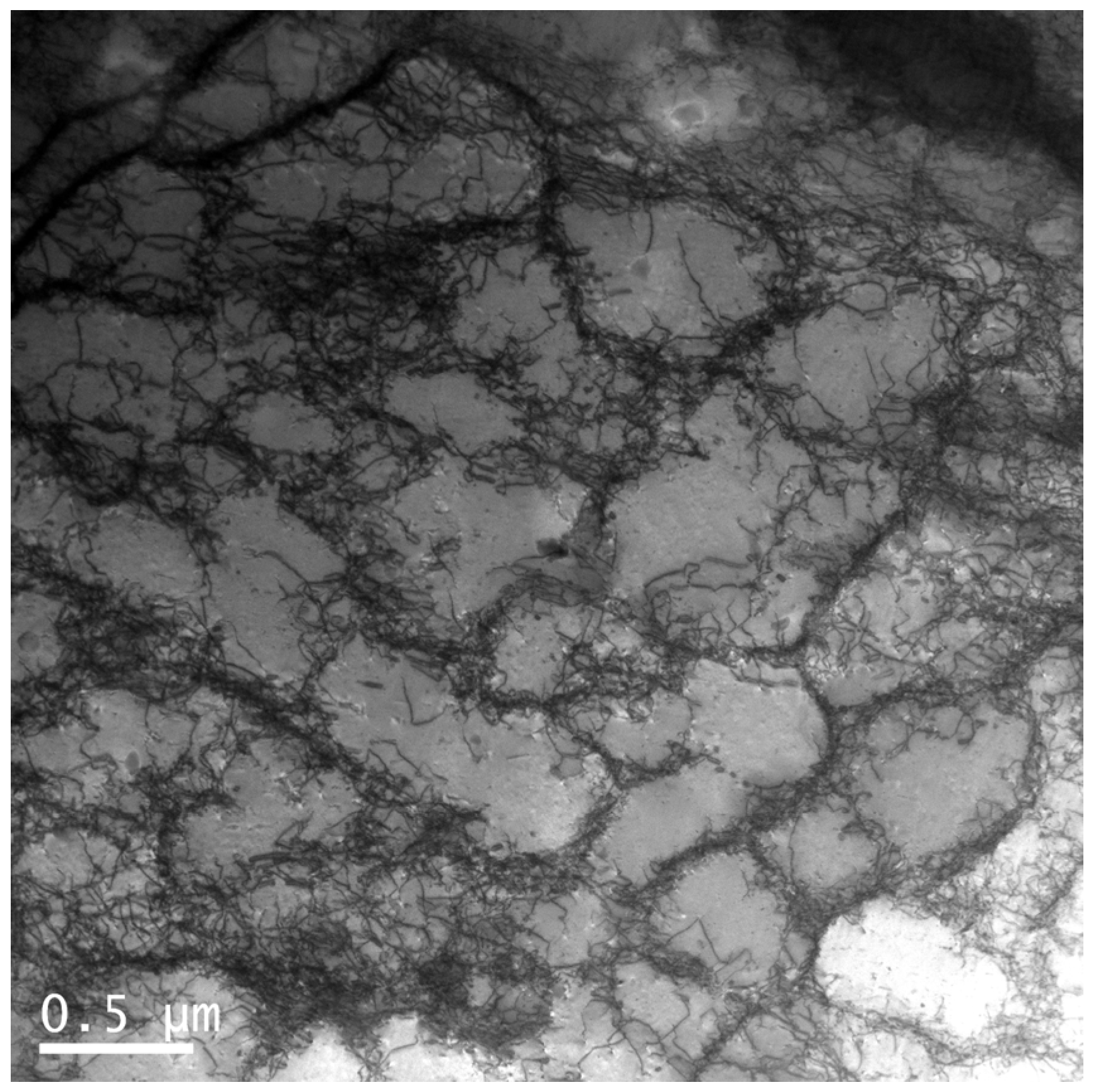
During plastic deformation, tangles of dislocations are created in practically all alloys. The tangles become thinner and more well-defined with increasing strain. Boundaries are formed that divide the materials into micron-sized cells or subgrains (see Figure 1). At high temperatures, the boundaries consist of a single layer of a dislocation network. These boundaries are referred to as subboundaries and the area they surround as subgrains. At ambient temperature, the boundaries are tangles of dislocations of finite width. They are called cell boundaries or walls because the regions they surround are referred to as dislocation cells or simply cells. Both cells and subgrains are said to represent a substructure. There is no sharp transition from cells to subgrains when the temperature is raised. Expressed in simple terms, cells are formed in the work hardening range and subgrains are formed in the creep range [1]. Many features are common for cells and subgrains. Hence, it is often natural to talk about properties of the substructure. Already at modest strain, the substructure is well developed in many materials. This means that the substructure can be observed in ordinary tensile and creep tests. At high temperatures, the substructure formation can be delayed. A planar dislocation structure with pile-ups can appear, for example, in some austenitic stainless steels or only a random network of dislocations, as in Al-Mg. As sufficiently high strains, a pronounced substructure is also found in these materials [2].
There are a number of excellent reviews on substructure in the literature [2,4,5]. In many cases there is no need to distinguish between cell and subgrain structure. For example, the stress dependence of their size is the same. Early on, the question was raised as to whether the substructure contributes to the creep strength [5,6]. Several authors argued that there was no contribution from the subboundaries. For example, Orlova found that the full creep strength could be accounted for by the dislocations in the subgrain interiors [7]. However, with the event of Mughrabi’s composite model [8], the situation changed. In the composite model, the subboundaries are considered as “hard” zones. In this model the strength is taken as a weighted average of the contributions from the hard zones and from the “soft” subgrain interiors. It has been verified experimentally that long range stresses exist from subboundaries [9]. In a single phase alloy, the subgrain size and its dislocation content are fully controlled by the applied stress and its strength contribution cannot be changed [5]. However, the subgrain size can be stabilized by the addition of particles in the same way as for ordinary grains (Zener effect) [10]. This effect is extensively utilized in modified 9% Cr creep resistant steels. Due to the presence of M23C6 carbides, the subgrain growth can be limited and the strength from the subboundaries can be kept [11].
Many studies on the formation of substructure are available, but few of them are quantitative. The work by Blum and Strauss is a notable exception where measurements of the subgrain size during creep in Cr-Mo steels were made [12,13,14]. Using these results and the model for the influence of particles on subgrain growth [10], the creep rupture strength of 9–12% Cr steels at long times could be understood [11].
If dislocations on a given slip plane in a cell are considered, dislocations with opposite Burgers vector or orientation move in opposite directions under an applied stress. Such dislocations are said to have different signs. This means that dislocations with different signs end at different positions in the cell. As a consequence, they are found at different sides of the cell boundaries in the stress direction. These dislocations are referred to as unbalanced or polarized, since the Burgers vectors and orientations are not homogenously distributed. Most of the dislocations are still characterized with an equal distribution of b and −b Burgers vectors and orientation at the cell boundaries, providing a barrier between polarized dislocations. The dislocations with a homogenous distribution of signs are called balanced. Balanced or unbalanced dislocations should not be confused with geometrically necessary dislocations that are formed to accommodate plastic strain gradients in the crystal, for example around coarse particles. Balanced and unbalanced dislocations are statistically stored dislocations that are created by work hardening.
Creep is a form of plastic deformation that takes place at constant load or stress. During deformation there is continued generation of dislocations due to work hardening. If work hardening would be the only process, the dislocation density would quickly reach a sufficiently high level so that the deformation would stop. This is what happens for most alloys at ambient temperatures. The reason why the straining during creep can continue is that dislocations are annihilated due to recovery. Dislocations of opposite Burgers vectors attract each other and when they meet they eliminate each other. This process is referred to as static recovery. If unbalanced dislocations are present, the rate of static recovery is reduced. Expressed in another way, the creep strength is enhanced.
The role of unbalanced dislocations is not widely covered in the literature, but it is of major importance for several properties. Basic models for tertiary creep have only recently been established [15]. It turns out that the unbalanced dislocations can match the applied stress during secondary creep, but are not able to do that during tertiary creep, which gives rise to the observed increase in the creep rate. Cold work can reduce the creep rate by several orders of magnitude. According to the common creep recovery theory, cold work does not influence the secondary creep rate at all, because the same limiting stationary dislocation density is always reached. However, by taking unbalanced dislocations into account, the raised strength can be clarified. For copper, it has been possible to quantitatively explain why cold worked copper can have six orders of magnitude lower creep rate than soft copper [16].
Most creep tests are carried out at constant load. The interpretation of the results is in general made in terms of the nominal stress, not the true stress. This is no major problem at high temperatures, when the stress exponent for the secondary creep rate is about 5. However, at lower temperature, when stress exponent can be 30 to 50, the difference between nominal and true cannot be ignored. For example, for copper at 75 °C, the stress exponent exceeds 50. For a strain of 0.2, the ratio between the creep rate given by the true and the nominal stress is more than a factor 10,000. Surprisingly, the creep curves at 75 °C look very much like those at a much higher temperature. It took a long time to explain this effect, but it is due to the presence of unbalanced dislocations. They represent a massive back stress that can fully balance the enormous difference between the true and nominal creep rate [17].
In this paper, new quantitative models for cell and subgrain formation are presented. The influence of the substructure on properties is analyzed. The focus is on properties where unbalanced dislocations play a major role. This type of dislocation has a dramatic effect on the appearance of creep curves and can explain the influence of cold work on the creep strength.
2. Modeling of Subgrain Formation
2.1. Strength from Dislocations
The Taylor equation is used to describe the influence of the dislocations on the creep strength σdisl
where ρ is the dislocation density, α a constant, mT the Taylor factor, G the shear modulus, and b the Burgers vector. When considering substructure, Equation (1) has to be modified because the contribution from cell walls is different from that of the cell interiors since the value of α is different. An equation for α derived by Kuhlmann-Wilsdorf [18] illustrates this:
νP is Poisson’s ratio and RCO a cut-off radius that is given by the spacing of dislocations. In the cell interior and the cell boundaries, this spacing is of the order 10−7 m and 10−8 m, respectively. This implies that α is twice as large for dislocations in the cell interiors in comparison with those in the cell walls. As a consequence, Equation (1) has to be replaced by
where ρint is the dislocation density in the cell interior and ρbound is the dislocation density in the cell boundaries. There is an expression for α that is adapted to high temperatures and the value of αKW will not be used here. Many measurements have been performed to determine the value of α. Unfortunately, there are large differences between different observations. Rather than picking one of the observations, a theoretical result is chosen. There is a short range part and a long range part of α. It is the long range part αG that is of importance at elevated temperatures and that is the value that is used here [19,20].
With νP = 0.3, αG takes the value of 0.19.
The cell and subgrain size dsub can directly be related to the stress
Ksub is a dimensionless constant that, for many metals, has values in the interval 10 to 20. Staker and Holt were the first ones to suggest an equation of the form of Equation (5) [21]. Following Kuhlmann-Wilsdorf, it is assumed that it is the dislocation stress and not the total applied stress that appears in Equation (5) [18]. Equation (5) is quite general and it has been proposed that it is also valid for non-stationary conditions when the stress varies [22]. There are two well-known derivations of the relation between the subgrain size and the stress. Staker and Holt based their derivation on an unstable set of parallel screw dislocations [23]. In the second derivation, the energy of a substructure was taken as the sum of the dislocation line energy and the dislocation cell stresses. The sum of these two contributions was minimized, resulting in Equation (5) [18].
The distance between the dislocations in the cell walls or subgrain boundaries is called the dislocation separation. With some simple assumptions, this distance can be estimated. A subgrain boundary is considered to consist of a single layer with μ sets of dislocations. μ is typically 2 or 3. If the cells are arranged as packed cubes, the following relation is obtained:
where lsep is the dislocation separation. Three cubes sides are associated with each corner in the cube structure. This is the origin of the factor of 3 in Equation (6). The density is defined as the average over each cell with a volume of dsub3. This estimate of the dislocation separation, with the help of Equation (6), will be compared to observations below.
2.2. Formation of Subgrains during Creep
In the secondary stage, most alloys have a well-defined substructure. However, there are exceptions. At around 300 °C, subgrains are not present in AlMg until a strain of about 1 [2]. Furthermore, a planar dislocation structure can be found in some austenitic stainless steels. For 17Cr12Ni2Mo, subgrains were found at 704 °C but not at 593 °C [24]. An increased content of N can also reduce or remove the subgrains for 17Cr12Ni2MoN [25]. A simple explanation to these observations is that the stacking fault energy γSFE plays a role. There is a pronounced increase in γSFE with temperature for 17Cr12Ni2Mo and that could be the origin of the findings in [24]. It should be pointed out that it is quite unusual that γSFE increases with temperature. For some austenitic stainless steels, it is a consequence of change of the magnetic structure with temperature. There are many results for the effect of N on γSFE for ordinary austenitic stainless steels, but the observations are far from unanimous. A recent study where the available information has been penetrated [26] proposes that N reduces γSFE and this can explain the findings for 17Cr12Ni2MoN [25]. The presence Mg clearly lowers the value of γSFE in Al-alloys, but whether that is of importance for the delay of subgrain formation in Al-Mg alloys is not known.
Before the modeling of the subgrain formation can be performed, the creep model that is to be used must be presented. A basic model will be applied. Only a brief summary of the model is given, because it is derived and described in detail elsewhere [27]. The starting point is the development of the dislocation density ρ during creep and other types of plastic deformation
where ε is the strain, the strain rate, mT the Taylor factor, b Burgers vector, cL a dimensionless factor, ω the dynamic recovery constant, τL the dislocation line tension, and M the dislocation climb mobility. The three terms on the right-hand side (RHS) of Equation (7) describe the effect of work hardening, dynamic recovery, and static recovery. During stationary creep, the dislocation density is constant and the creep rate can directly be obtained
where σ is the applied stress, and G is the shear modulus. σdisl is the dislocation stress and ρ the dislocation density. σi is an internal stress that is primarily due to solid solution and particle hardening. It has been demonstrated that Equation (8) can describe the creep rate over a wide range of temperature and stresses for a number of materials [27]. In addition to the secondary creep rate, the primary creep rate is also needed to model the subgrain formation. Once the stress dependence of the secondary creep rate is known, the creep rate in the primary stage can be obtained directly [17].
Thus, primary creep can be described with an effective stress σeff
At the start of creep for an annealed material, σdisl is small and the creep rate is very high. During primary creep, the dislocation density and consequently also σdisl increase rapidly. Eventually, the secondary stage is reached. Equation (10) is satisfied and Equation (8) is recovered. Therefore, Equation (8) is a special case of Equation (11). It has been shown that Equation (11) reproduces the observed time and strain dependence in the primary stage [17]. The limitation of Equation (11) is that it cannot the model creep rate at very small strains, but that is no of importance in the present paper. Furthermore, there are models that can describe the behavior at small strains [28].
The normal case where subgrains are present in the secondary stage will now be considered. Blum and co-workers investigated the subgrain formation in Al5Zn at 250 °C and a stress of 16 MPa [2,29]. Zn gives rise to solid solution hardening. It can be described by a solid drag effect [30].
νclimb is the dislocation climb speed, ci0 is the concentration of solute i, and Di the diffusion constant for solute i, kB Boltzmann’s constant and T the absolute temperature. I(z0) is an integral of z0 = b/r0kBT where r0 is the dislocation core radius. The climb speed and the solute–dislocation interaction parameter β are given by
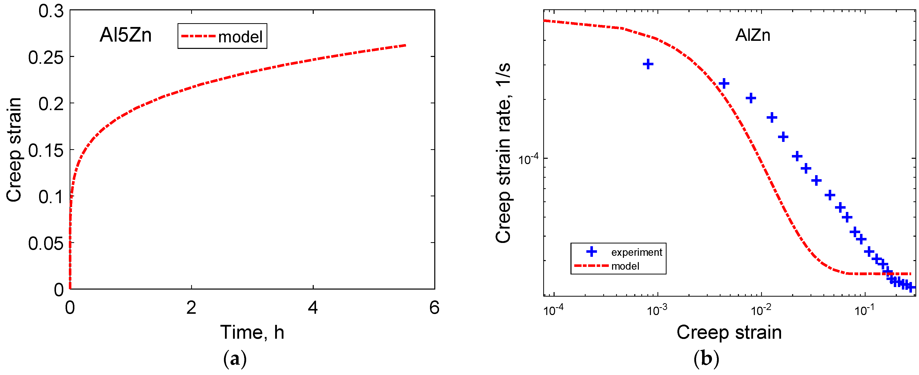
δi is the linear misfit parameter which is −0.02 for Zn in Al. The resulting value of the solid solution hardening σi is 4.6 MPa. For h(σ) in Equation (8), values for Al are applied [31]. The computed time dependence is given in Figure 2a and the creep strain rate versus strain is shown in Figure 2b.
Before the secondary stage is reached, both the model and the observations follow an approximately straight line, although the slopes are not identical. This type of behavior with a straight line in a double logarithmic diagram is referred to as the ϕ-model. It is a characteristic feature of many materials [28].
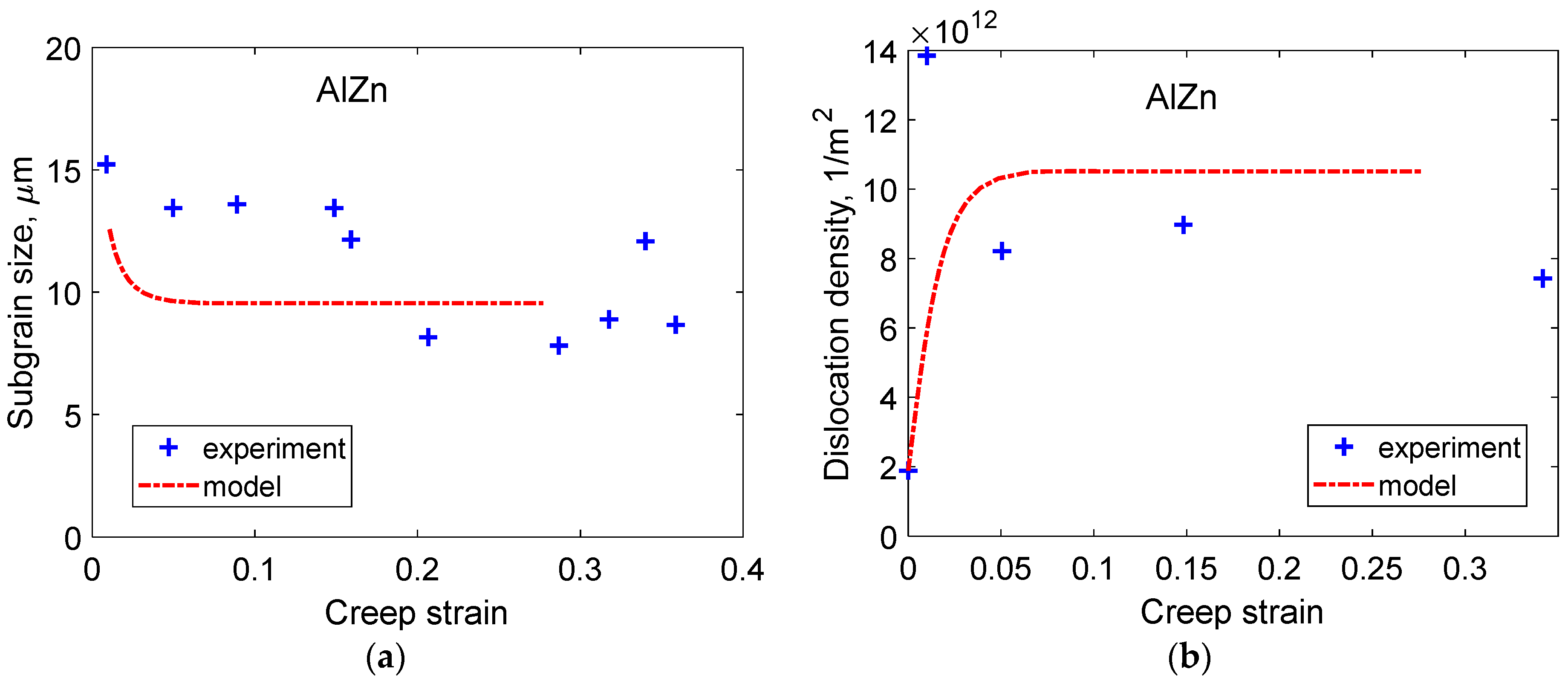
The creep rate is controlled by the effective stress according to Equations (11) and (12). It is now assumed that also the subgrain size is determined by the effective stress. Thus, by combining Equations (5) and (12), a simple model for the subgrain size can be obtained. The results are illustrated in Figure 3a.
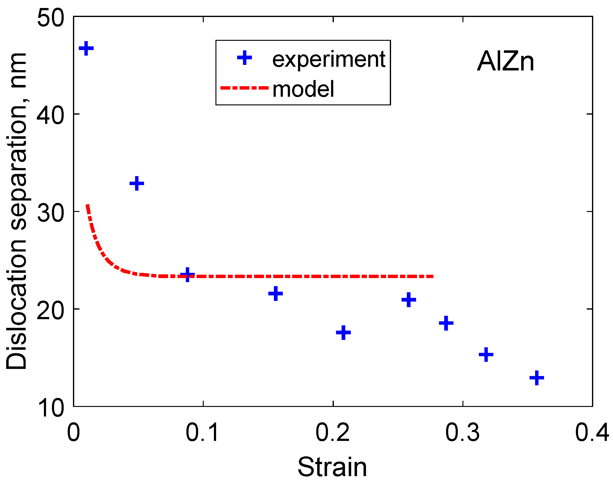
The strain dependence of the dislocation density can also be derived with the help of Equation (10). The predictions are given in Figure 3b. Now when the dislocation density has been determined, the dislocation separation can be computed with the help of Equation (6). Most of the dislocations are assumed to be located in the subgrain boundaries. The model values are compared to the experiments in Figure 4.
2.3. Cell Formation at Constant Strain Rate
During tensile and compression testing at ambient temperature, dislocation cells are created in virtually all alloys. Koneva et al. [32] has made a brief review of cell formation. The cell diameter is reduced with increasing strain in the same way as for creep. They found that the cell diameter was inversely proportional to the square root of the dislocation density
This is fully consistent with Equations (5) and (10). Equations (3), (5) and (16) gives
where μsub = 1 and 2 for dislocations in the subgrain interior and walls, respectively. For Cu, a value of Krho = 15 was obtained. This figure is reasonably consistent with the commonly found value of Ksub = 10. For alloys, Koneva et al. found considerably smaller values: Krho = 2 to 5 for Cu-Al and for 2 to 5 for Cu-Mn. This is an indication that Ksub can be smaller for alloys than for pure metals. Koneva et al. also collected values from earlier investigations, but they do not seem to be in agreement with more recent findings.
As pointed out, the above subgrain boundaries are in general considered to be built up by one layer of dislocations. However, cell walls have a finite width wcell. Then, Equation (6) has to be replaced by
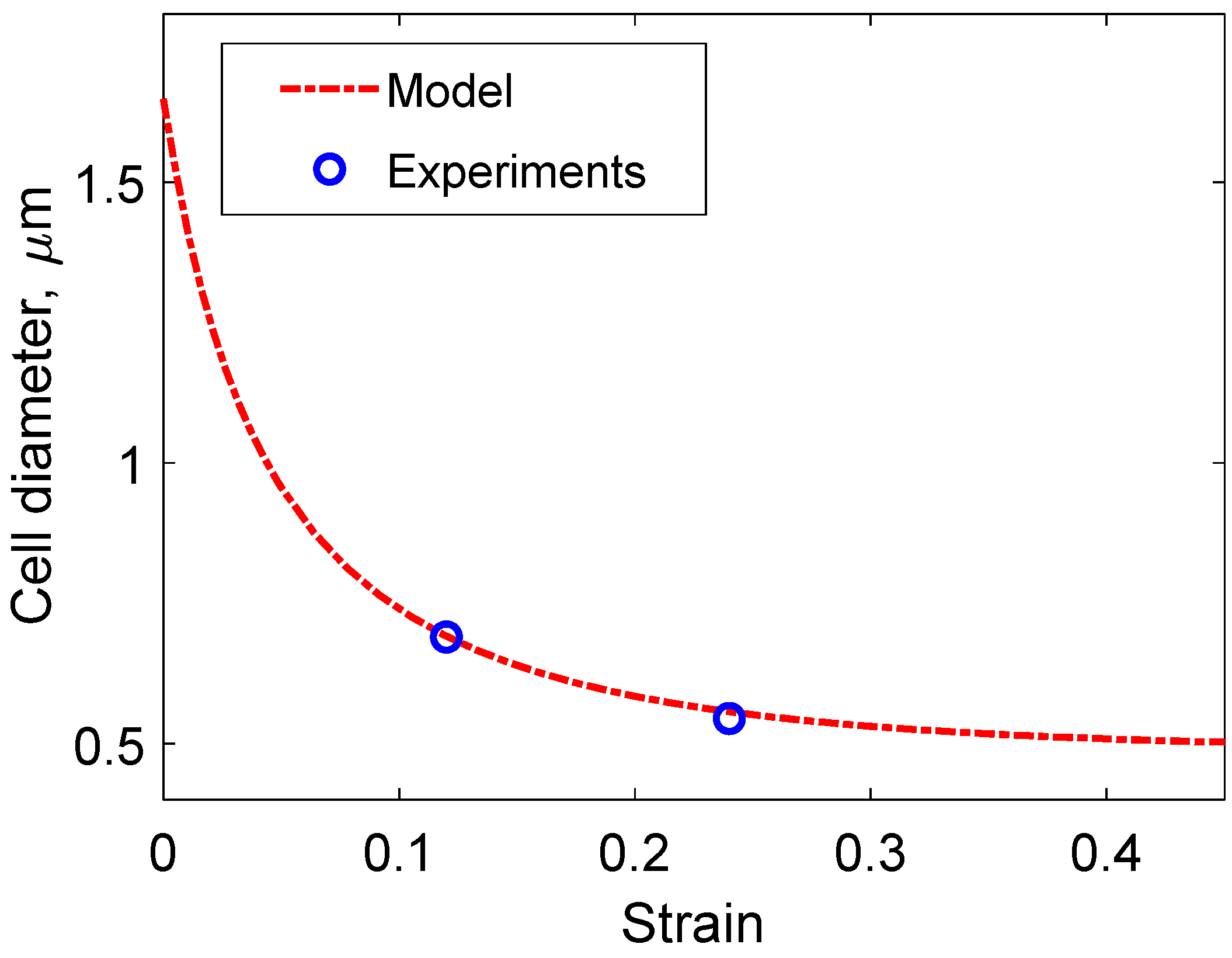
The separation distance in Equation (18) is assumed to be same along the cell boundary and perpendicular to it. In the boundaries, several types of dislocations have to be considered [16]. Equations for the development of each dislocation type will be given in Section 3. Once the strain dependence of the dislocation densities has been established, the dislocation stress can be computed with Equation (3) and the cell size with Equation (5). Results for the influence of the creep strain on the cell size are illustrated in Figure 5. The cell size is reduced with increasing strain and tends towards a stationary value.
Dislocation locks are formed in the boundaries, which are stabilized by the locks. The locks are believed to be dominated by Cottrell–Lomer locks, which are built up of immobile partial dislocation configurations [33]. It has been assumed that the width of the cell boundaries is related to the density of locks ρlock [16].
If Equations (18) and (19) for the dislocation separation and wall width are combined, they can explicitly be expressed in terms of the dislocation densities
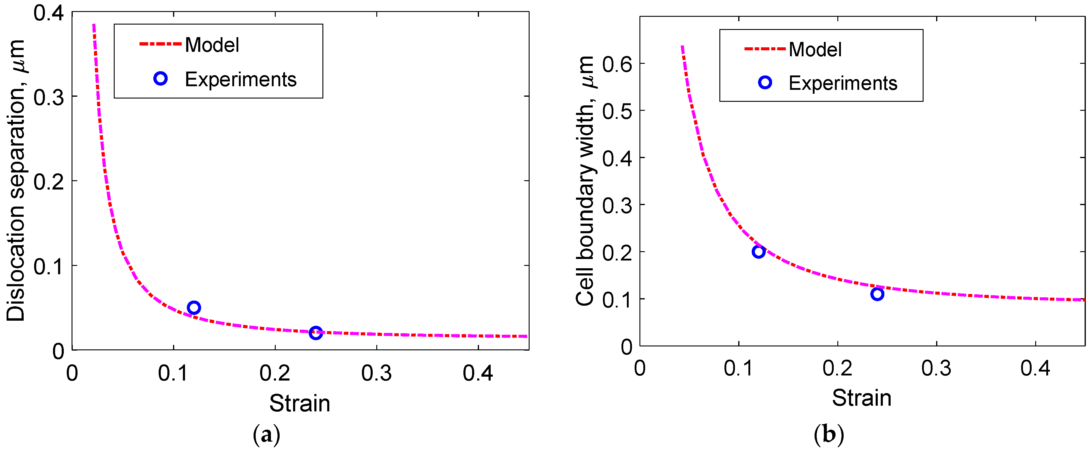
These equations are compared to experimental data in Figure 6.
The dislocation separation and the wall width decrease with increasing strain in a similar way that was observed for the cell size in Figure 5. However, the rate of the decrease is more rapid than in Figure 5. These findings are not consistent with those of Koneva et al. [32]. They proposed a constant ratio between the cell diameter and the boundary width.
In [2], measurements of the substructure as a function of strain for a 18Cr8Ni austenitic stainless at 865 °C at constant strain rate are presented. The subgrain size and the dislocation separation decreased with increasing strain in the same way as for Cu-OFP. There was a rapid increase in the dislocation density with increasing strain, which leveled off to a stationary value. We attempted to use the dislocation model to simulate this behavior. Unfortunately, the published stress strain curve was not consistent with the model.
3. Influence of Cold Work on the Creep Rate
For an annealed material, the low initial dislocation density increases rapidly during primary creep and tends towards a stationary value in the secondary stage. This behavior can be represented by Equation (7). With the help of this equation and Equation (11), the creep rate during the primary stage can be computed. It has been demonstrated that the observed behavior can be described quite well [17,28]. For cold worked material, on the other hand, the initial dislocation density is high and according to Equation (7) it would reach the same stationary value as for annealed material. This is the consequence of basic creep recovery theory. However, this is not in accordance with observations. For example, for austenitic stainless steel, cold work can raise the creep strength significantly [34,35,36,37]. For a review, see [38]. The increase in creep strength is not observed under all conditions. If the temperature is too high or the cold work strain is too large, the microstructure can become unstable and the material may recrystallize. The effect of cold work on the creep strength was for a long time a major puzzle in the theory of creep that has only recently been clarified.
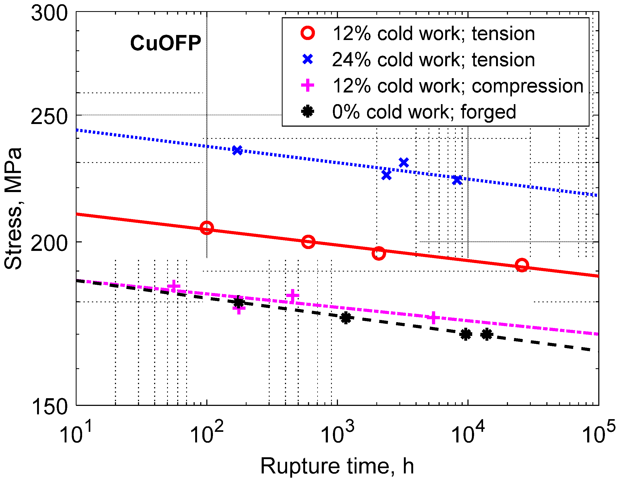
The effect of cold work on the creep strength of Cu-OFP (Cu with 50 ppm P) will be analyzed in this section. In Figure 7, observations for creep rupture data are given.
Results are shown for 0%, 12%, and 24% cold work. The effect of cold work is quite dramatic. 12% cold work raises the rupture time by three orders of magnitude and 24% by six orders. Only if the cold work was carried out in tension would these large increases be observed. With cold work in compression, only a small effect on the rupture time was found. The creep testing was performed in tension. Thus, if the cold work and the testing were made in the same direction, a major effect of the cold work was recorded, but not if the direction of cold work was reversed.
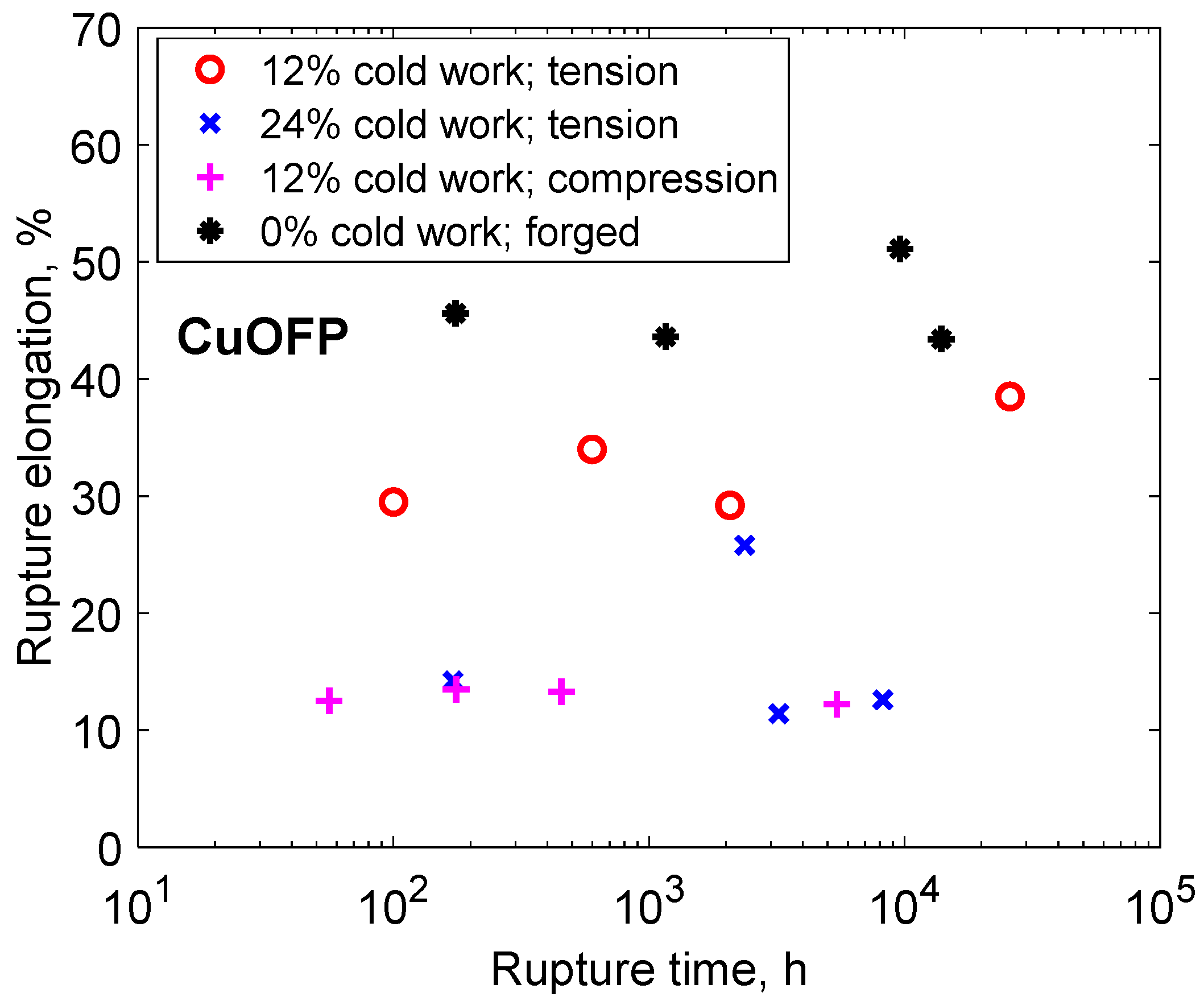
The creep ductility is typically reduced with increasing amounts of cold work. This is clearly observed for Cu-OFP as well (Figure 8).
For Cu-OFP in a soft condition the creep ductility is quite high, about 40%. For 12% cold work, the ductility is still high, about 30%. For 24% cold work, the ductility takes values just above 10%. For 12% cold work in compression, the ductility is modest, in spite of the fact that the increase in creep strength is limited.
The effect of substructure must be considered to explain the influence of cold work [16]. This has also been proposed in the literature, but without providing any analysis that could explain the magnitude of the influence [4,39]. As was summarized in Section 1 and Section 2, a substructure was formed during deformation in almost all alloys. The dislocations move towards the subboundaries, and in this way the substructure is created. However, all dislocations do not move in the same direction. Dislocations with opposite Burgers vectors or orientation flow in opposite directions. This is evident from the Peach–Koehler formula
where F is the force on a dislocation with direction ξ and Burgers vector b. By changing the sign of the Burgers vector, the sign of F is reversed. As a consequence, dislocations with different Burgers vectors move to different positions at the boundaries. At the two sides of a boundary, the dislocations tend to have different signs. The dislocations become polarized. All of the dislocations are not polarized, but the outer layers of the boundaries are assumed to be.
The presence of polarized dislocation has a major effect on the rate of recovery. Since dislocations of opposite signs are not available amongst polarized ones, static recovery cannot take place. Polarized dislocations are also called unbalanced and unpolarized dislocations for balanced since matching are not present and present for them, respectively.
The cell and subgrain boundaries are assumed to consist of three types of dislocations: balanced, unbalanced, and locks with densities of ρbnd, ρbnde, and ρlock. The dislocations are mainly located in the boundaries and the ones in the cell interiors are neglected. The equations for the different types of dislocation are given in Equations (23)–(25) [16].
In Equation (23) for balanced dislocations, work hardening, dynamic recovery, and static recovery are considered in the same way as in Equation (7). The inclusion of the factor kbnd is the only difference. The reason is that the Taylor Equation (3) has been modified in relation to the common formulation in Equation (1). If only balanced dislocation is present, Equation (23) should give the same result as Equation (7). The equation corresponding to (23) for unbalanced dislocations is
There are two important differences between Equations (23) and (24). There is no term for static recovery in Equation (24). This is the result of the absence of matching dislocation that was discussed in detail above. The second difference is that both unbalanced and unbalanced dislocations contribute to the generation of unbalanced ones, since both types move across the cell interiors in a similar way.
The second term on the RHS of Equations (23) and (24) represents dynamic recovery. This type of recovery is, for example, of major importance for stress strain curves at ambient temperatures. If dynamic recovery is not taken into account, stress strain curves would be straight, which is certainly not what is observed. Dynamic recovery reduces the work hardening rate with increasing strain. In the modeling of dynamic recovery, it is usually assumed that dislocations with opposite Burgers vector are annihilated when they are close enough [40]. With this description, the mechanism is very close to that of static recovery. The problem is that these two recovery mechanisms have very different temperature and time dependence. Dynamic recovery is only weakly temperature dependent, whereas static recovery is proportional to the self-diffusion coefficient with quite a strong influence of temperature. In addition, dynamic recovery is strain dependent and static recovery time dependent.
To resolve these difficulties, Argon has suggested that dynamic recovery is due to what happens when the dislocations generated during work hardening pass through cell boundaries [33]. It is known that each generated dislocation travels a distance of about 3 cell diameters [41], so it clearly crosses cell boundaries. Dislocations will be removed and low energy configuration will be formed when the dislocations penetrate the cell boundaries. Some of these low energy configurations are Cottrell–Lomer locks. This mechanism gives a possible explanation for the observed temperature and strain dependence of dynamic recovery. The strain dependence of the lock density ρlock can be described by the following equation [16]
The formation of locks has contribution from both balanced and unbalanced dislocations. The locks are exposed to both dynamic and static recovery; dynamic recovery since the dislocations passing through the boundaries remove locks; static recovery, since when climb takes place even complex dislocation configurations reduce the energy content and their number of dislocations.
Experimental stress strain curves can be accurately reproduced with the help of Equations (7) and (10) [42] with a homogenous distribution of dislocations. If the dislocations are to be assumed to be located in the boundaries, it should be possible to simulate the stress strain curves with Equations (23) and (25) combined with Equation (3). The resulting curves should be the same. This is the case with kbnd = and kbnde = . The value of klock is smaller. A value of 0.1 has been chosen. With these constants, the curves in Figure 5 and Figure 6 are obtained.
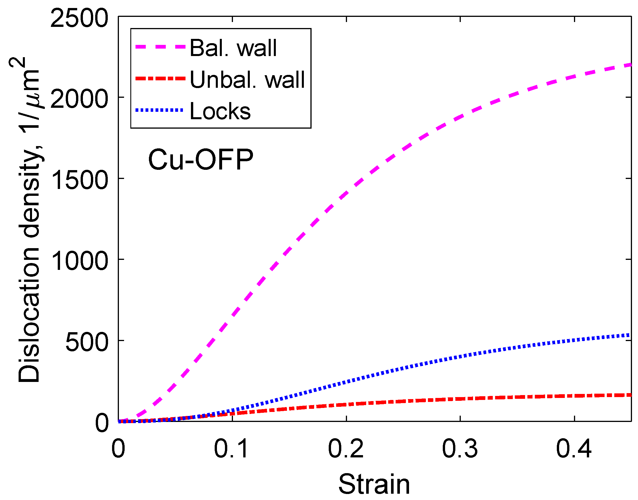
The influence of cold work in Figure 7 will now be considered. At ambient temperature, cold work of 12% and 24% gives flow stresses of 201 and 241 MPa, respectively. If the dislocations are mainly located in the boundaries, which is what the observations suggest [3], and using Equation (3), the stress values correspond to total dislocation densities in the cell walls of 8.7 × 10¹⁴ and 1.5 × 10¹⁵ 1/m2. The dislocation densities are assessed as average values over the volume of the cells. The development of the dislocation densities with strain is shown in Figure 9. The balanced dislocation content dominates in Figure 9.
For the influence of the cold work, the unbalanced dislocation content ρbnde plays an important role. The reason is that it is not exposed to static recovery. The presence of a back stress σback reduces the creep rate
For undeformed material, the secondary creep rate is given by Equation (8). For cold worked material, Equation (8) is still applicable, but with σback as a major contribution to σdisl according to Equation (3). From the 50 ppm alloying with P in Cu-OFP, there is a contribution to σi from solution hardening of about 20 MPa at 75 °C [27].
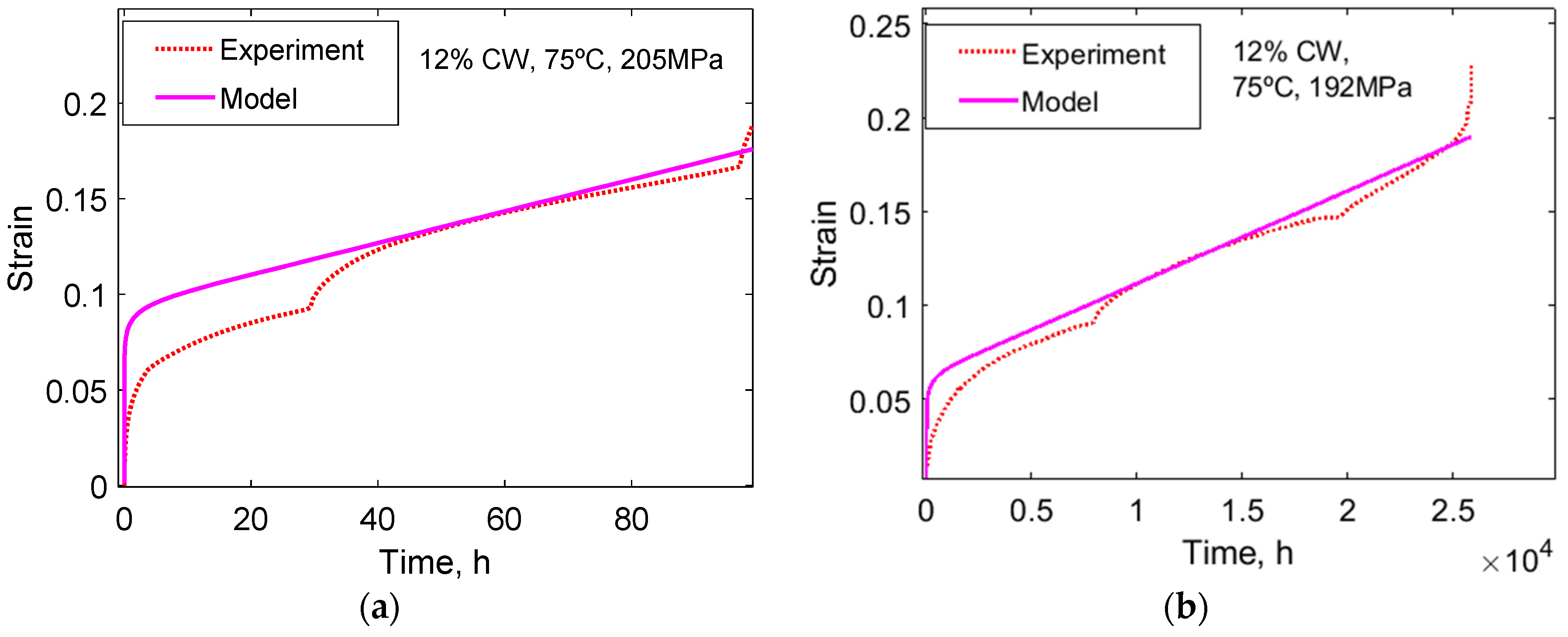
The validity of Equation (11) and its time integral has been demonstrated for Cu without cold work in [17]. Creep strain curves for 12% cold-work Cu-OFP are illustrated in Figure 10.
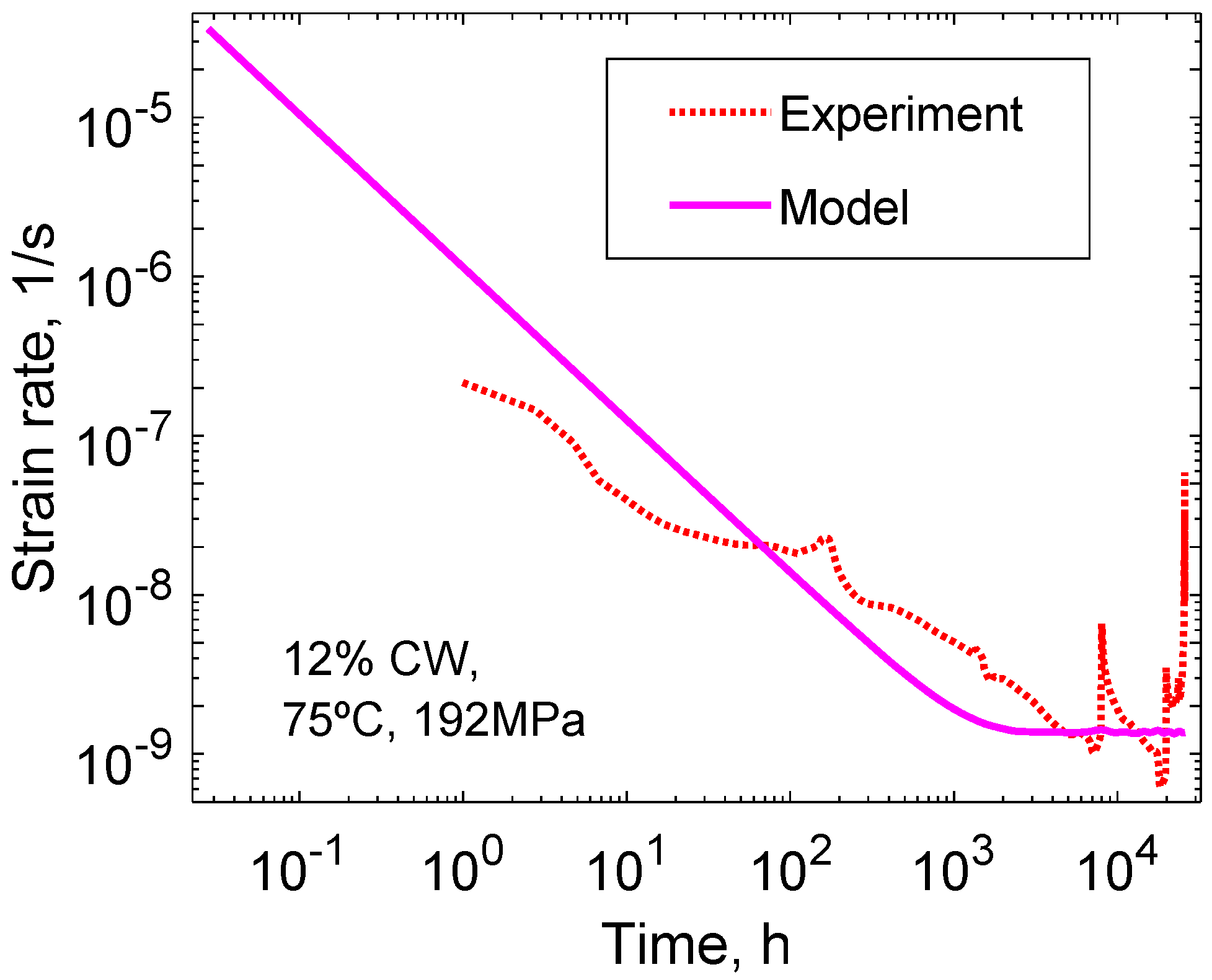
Distinct primary and second creep are present in Figure 10. The strain during primary creep is somewhat exaggerated in the model. The creep rate in the secondary creep rate is well reproduced. It should be noticed that the creep rate is three orders of magnitude lower than for soft Cu and it can still be accurately represented. This is a result of the lower recovery rate of the unbalanced dislocations. The observed amount of tertiary creep is limited. The tertiary creep that is present is probably due to necking. It is possible to take it into account in the model [15], but that is not done in Figure 10. The creep rate versus time for the second case in Figure 10 is shown in Figure 11.
In Figure 11, the slope of the curve in the primary stage is constant. The author refers to this behavior as the ϕ-model. It is observed for many types of materials without cold work, cf. Figure 2b and Figure 15 below [28]. Evidently, it is at least approximately applicable to cold worked material as well. The drop in the strain rate with time Figure 11 is quite dramatic. The drop is typically much larger than for soft material, a fact that the model can cope with [17].
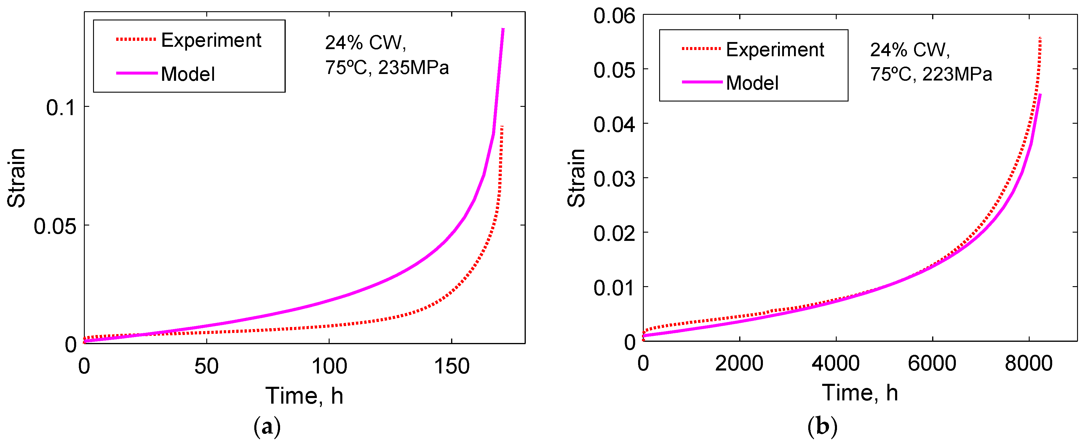
Creep strain versus time curves for 24% cold deformed Cu-OFP are given in Figure 12.
In Figure 12, the creep rate is about six orders of magnitude lower than for soft copper. The model can evidently simulate these low creep rates. If Figure 10 and Figure 12 are compared, it is clear that the creep curves are very different for 12% and 24% cold work. For 12% cold work, secondary creep is dominating the creep curves and the amount of tertiary creep is limited. For 24% cold there is no primary creep and only limited secondary creep, and the main part of the creep curves is due to tertiary creep. In spite of the difference, the model can reproduce the creep curves in Figure 12 in a reasonable way. For 24% cold work in comparison to 12% cold work, the cell size, the cell wall width, and the dislocation separation are smaller, see Figure 5, Figure 6 and Figure 7. The gradual increase in the creep rate for 24% cold work is due to enhanced recovery.
By taking a back stress from the unbalanced dislocations into account, according to Equation (18), it can be summarized that many of the features of creep of cold worked copper can be described. The creep rates are three and six orders of magnitude lower after 12% and 24% cold than in the soft condition. For both degrees of cold work, the whole creep curves can be simulated in an acceptable way in spite of their differences. The presence of unbalanced dislocations can also explain why the effect of cold work essentially disappears when the cold work is performed in compression and the creep testing takes place in tension. When the loading direction is reversed, the unbalanced dislocations move away from the boundaries and no back stress appears.
It has been assumed above that it is the stabilized substructure due to the presence of unbalanced dislocations that is the main origin of the effect of cold work on creep. The substructure can also be stabilized with the help of particles. The most well-known case is for modified 9%Cr steels, where long term creep strength is improved by locking the subboundaries with M23C6 carbides [43]. It is well established that cold work can improve the creep strength fort austenitic stainless steels. One mechanism that has been suggested is that the movement of subboundaries could be reduced due to the presence of particles, but detailed analysis of the effect has not been carried out [34,35].
4. Formation of a Dislocation Back Stress
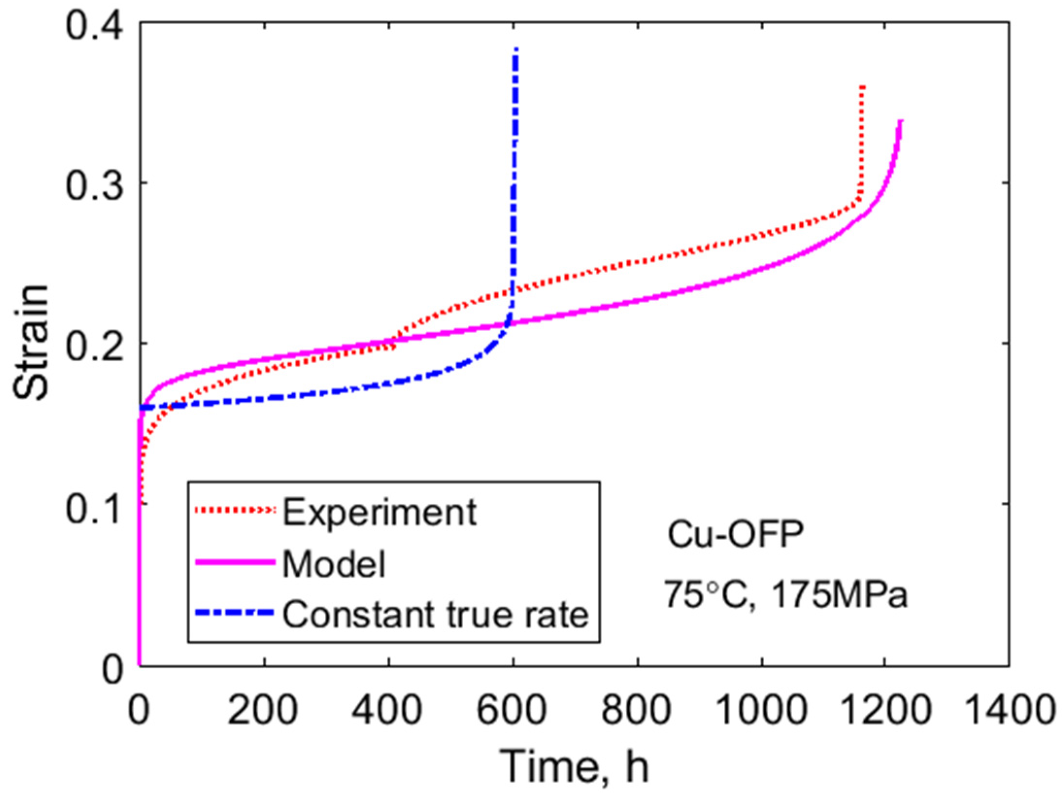
A creep curve for Cu-OFP in a forged condition (soft) at 75 °C is shown in Figure 13. Distinct primary, secondary, and tertiary stages are evident. The creep curve looks much the same as at much higher temperatures at about half the melting point, and that is a typical feature for copper at near ambient temperatures.
This might not seem very surprising but it has very important technical consequences. When modeling secondary creep, for example, with finite element software (FEM), it is usually assumed that true strain rate is constant. Next, we will illustrate what happens if this starting point is used. For simplicity, it is illustrated with the help of a Norton equation so that the creep rate can be represented with a power law relation
where A0 is a constant and σ0 is the nominal applied stress. In Figure 13, the stress exponent nN is about 70. The creep test was performed at constant load. To take into account the effect of the reduction of the specimen cross section during the test, the factor eε is introduced. In this way, the stress is changed from a nominal to a true value. The parameters in Equation (27) are set in the following way. The starting strain of the creep curve is put as ε0 = 0.17 to be able to handle the role of primary creep to some extent. The Norton creep curve is furthermore assumed to cross the experimental curve at 600 h by choosing the value of A0. The resulting curve is illustrated in Figure 13. It is evident that the Norton curve has no resemblance to the experimental curve. It can be concluded that an expression with a constant true strain rate cannot describe the creep strain behavior. It is easily verified that the choice of values of the parameters A0 and ε0 do not affect this conclusion.
The strain rate in Equation (27) is strongly influenced by the factor exp(nN ε). For example, for ε = 0.1 this factor is 1100. The magnitude of this factor gives an extremely rapid increase in the strain rate, an increase that has never been observed. An assumption of a constant true strain rate at near ambient temperatures for Cu in the secondary stage is fully inconsistent with observations.
To be able to model not only the primary and secondary creep but also tertiary creep, the expression for the effective stress in Equations (11) and (12) has to be modified
where σ is the true applied stress, σ is the nominal applied stress, σi is the internal stress, and σdisl is the dislocation stress. The true applied stress σ is related to the nominal stress as
In the expression for the dislocation stress, it is vital to take into account the back stress according to Equation (26), or more precisely according to Equation (3). The resulting creep curve is included in Figure 13. It will now be explained why this approach works.
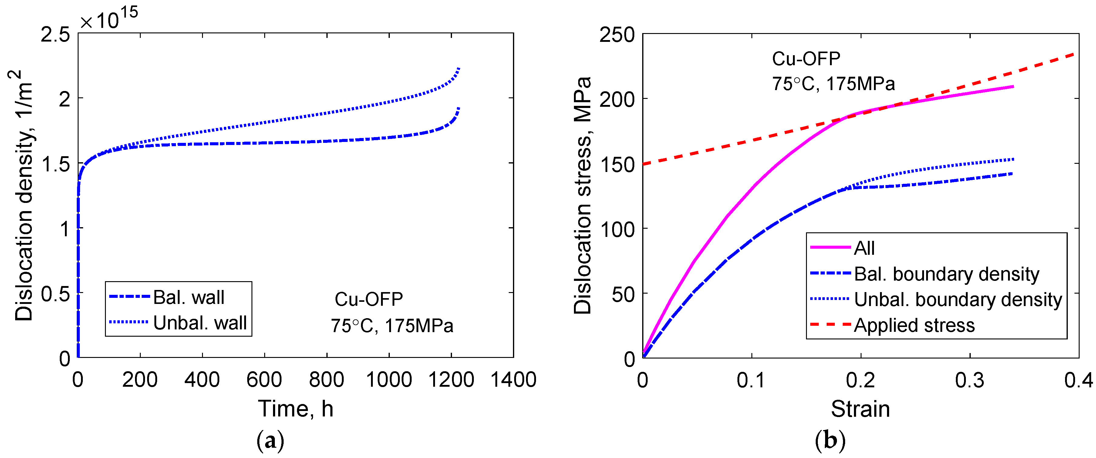
In Figure 14a, the dislocation densities ρbnd and ρbnde are given as a function of time. The densities are derived with the help of Equations (23) and (24). The resulting dislocation stresses versus strain are shown in Figure 14b using Equation (3). The stresses are illustrated for the balanced content ρbnd, for the unbalanced content ρbnde, and for the total content ρbnd + ρbnde. In this case, the small contribution from ρlock is ignored. The relation between ρbnd and ρbnde is not known. It is assumed that they are of about the same size. This gives kbnd = kbnde = .
In Figure 14a, the balanced dislocation density is approximately constant. However, the unbalanced content continues to increase in the secondary stage. How this influences the dislocation stresses is illustrated in Figure 14b. The total dislocation stress from both the balanced and the unbalanced content is marked as ‘all’. During the secondary stage, the total dislocation stress matches the true applied stress. In this way, the creep rate is prevented from increasing in an uncontrolled way. However, in the primary and in the tertiary stages, the true applied stress exceeds the total dislocation stress and consequently the creep rate is higher in these stages. The starting stress is 150 MPa, which is less than the applied stress of 175 MPa. The difference is the yield strength.
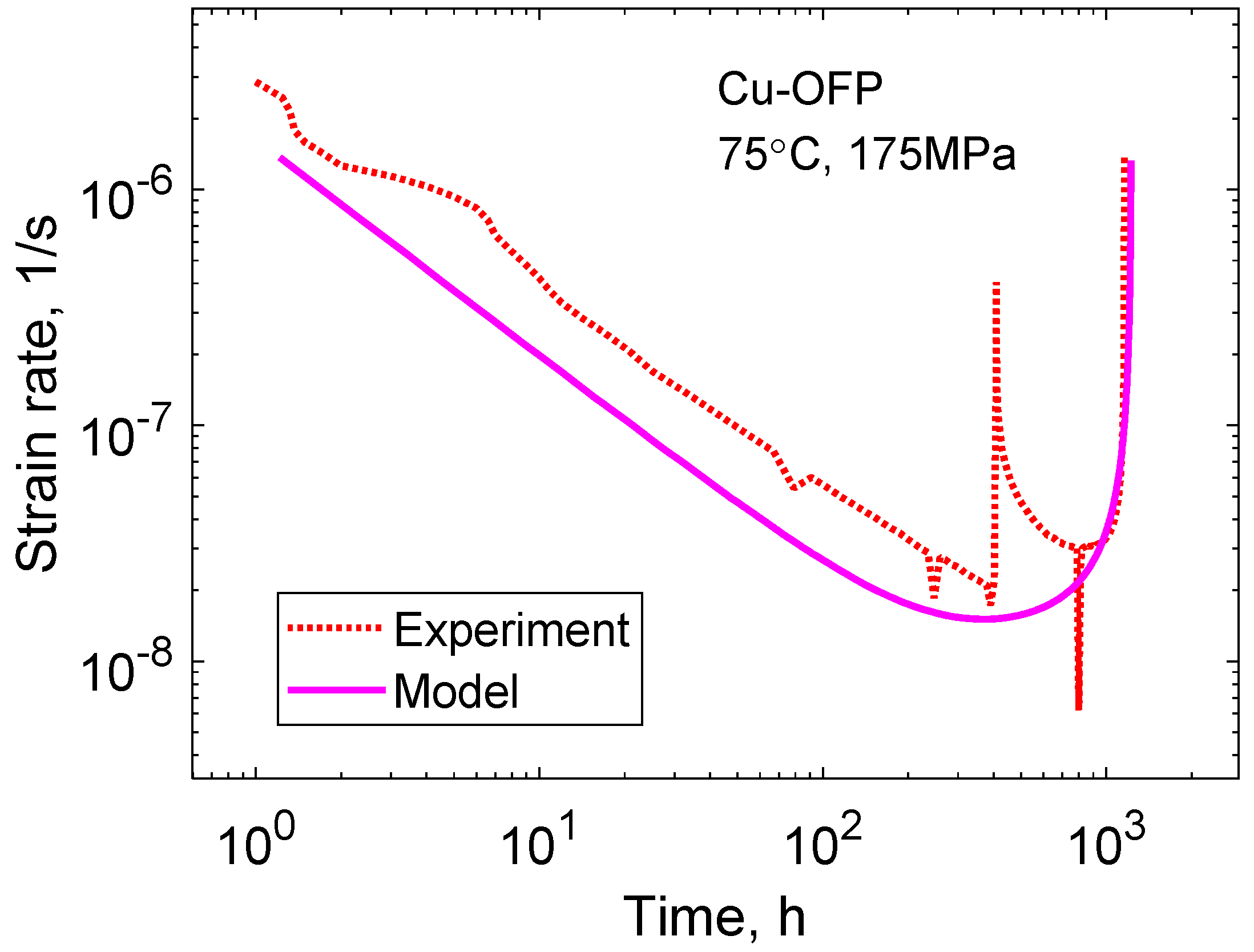
The whole creep curve in Figure 13 is reasonably described by the model, including tertiary creep. Another way of making a direct comparison with experiment is to consider the creep rate versus time curve. This is done in Figure 15.
Additionally, the creep rate version time is represented in an acceptable way. Both the primary and tertiary stages can be handled. However, the presence of cusps in the experiments makes a detailed comparison difficult.
It has been demonstrated that the presence of the back stress explains why the creep rate does not shoot off in the way that the true stress would suggest. In addition, due to the inclusion of a back stress, tertiary creep can be modeled.
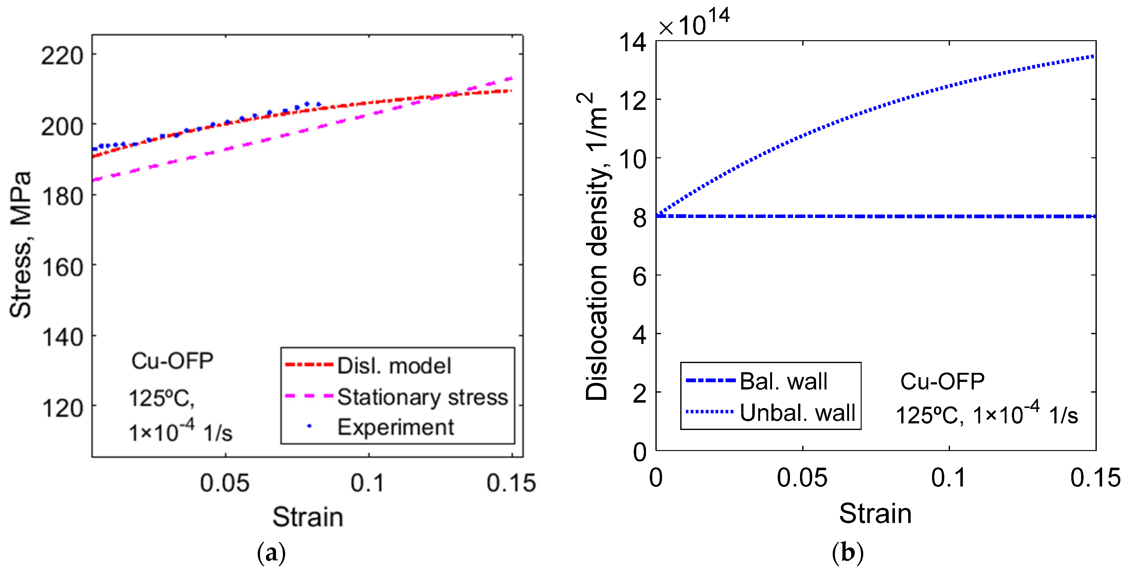
There also appears to be an effect of the back stress on stress strain curves from tensile tests at constant strain rate. In Figure 16, a case for 15% cold worked Cu-OFP at 125 °C is shown. A model curve using Equations (3), (23) and (24) is also illustrated.
It is assumed that the basic equation for the development of the dislocation density, Equation (7), is valid not only for creep but also for stress strain curves at constant strain rate. This means that the maximum stress in the stress strain curves is approximately given by the stationary creep stress at the same temperature and strain rate
where σstat0 and σstat are the nominal and the true stationary stress at 1 × 10⁻⁴ 1/s and 125 °C. The stress strain curves follows but are not identical to the stationary stress. The closeness of the curves verifies the principle.
The development of the balanced and unbalanced dislocation densities is shown in Figure 16b. Assuming that the balanced and the unbalanced densities are equal at zero strain, the values of kbnd and kbnde in Equations (23) and (24) can be fixed. For details, see [17]. It is evident from Figure 16b that the balanced dislocation density is constant, whereas the unbalanced content increases with strain. This increase explains how the flow stress can match the rise in the true stress.
According to the modeling and observations presented above, the back stress as defined in the analysis has a major impact on both creep and stress strain curves. It was shown that the effect is large for creep curves and cannot be neglected. This is of importance in stress analysis with finite element methods. There are two alternative ways to handle the situation. The first one is to compute the back stress explicitly by modeling the balanced and the unbalanced dislocation densities. However, this would require the development of special software. The other alternative is to replace the true stress σ in the stress analysis with σ∙exp(−ε). There is no major practical problem in doing this, but there is a psychological barrier because this is in direct contrast to what people have learned to do. However, neglecting the effect of the back stress would give rise to major errors.
The full effect of the back stress has only been demonstrated at near ambient temperatures for copper. However, the derivation is general and there are no assumptions that are specific for copper. Thus, the effect is likely to present in other materials as well. The effect of the back stress is likely to disappear at sufficiently high temperature because the unbalanced dislocation density cannot be expected to be stable any longer. Results for copper at 250 °C show that the effect is still there [44].
5. Summary
- At ambient or near ambient temperatures, dislocations form tangles that develop into cells during plastic deformation in practically all metals. In most metals, the cell structure is well developed after a strain of about 0.3. If higher temperatures are considered, subgrains are formed instead, consisting of a single layer of dislocations. Both the presence of dislocation cells and subgrains is referred to as substructure. If the stacking fault is low, a planar dislocation structure can be created instead of subgrains.
- There is a large amount of information on substructure in the literature. However, quantitative modeling of the development of substructure which is presented in this paper has only appeared recently. The presented modeling can describe data for Al-Zn and for copper.
- Dislocations with opposite Burgers vectors move in different direction during plastic deformation and end up at opposite positions at the cell walls. This implies that the dislocations have different Burgers vectors at the two sides of the cell walls. These dislocations are said to be unbalanced or polarized.
- The presence of unbalanced dislocations has a major impact on creep properties at near ambient temperatures and probably also at somewhat higher temperatures. Since unbalanced dislocations do not have matching ones with opposite Burgers vector, they are not exposed to static recovery. This gives a much more stable dislocation structure, and it is most likely the main reason why cold work can significantly raise the creep strength, in some cases by many orders of magnitude.
- For example, for copper, creep curves at near ambient temperatures have an appearance that is quite similar to that at much higher temperatures in spite of a high stress exponent. The high stress exponent would nominally give an enormous increase in the strain rate with increasing strain, but that is not observed. The reason is that the unbalanced dislocations create a back stress that counteracts the increase in the true stress. It is vital to take the effect of the back stress into account in stress analysis, for example, with finite element methods. Otherwise, the predicted creep rate can exceed the real one by many orders of magnitude.
Funding
Financial support from the Swedish Nuclear Fuel and Waste Management Co (SKB), grant number 25639 is gratefully acknowledged.
Institutional Review Board Statement
Not relevant for this study.
Informed Consent Statement
Consent was obtained from all persons involved in this study.
Data Availability Statement
Sources of data have been given in Figures captions and elsewhere.
Conflicts of Interest
The author declares no conflict of interest.
References
- Michel, D.J.; Moteff, J.; Lovell, A.J. Substructure of type 316 stainless steel deformed in slow tension at temperatures between 21° and 816 °C. Acta Metall. 1973, 21, 1269–1277. [Google Scholar] [CrossRef]
- MKassner, E.; Pérez-Prado, M.T. Five-power-law creep in single phase metals and alloys. Prog. Mater. Sci. 2000, 45, 1–102. [Google Scholar] [CrossRef]
- Wu, R.; Pettersson, N.; Martinsson, Å.; Sandström, R. Cell structure in cold worked and creep deformed phosphorus alloyed copper. Mater. Charact. 2014, 90, 21–30. [Google Scholar] [CrossRef]
- Bendersky, L.; Rosen, A.; Mukherjee, A.K. Creep and dislocation substructure. Int. Met. Rev. 1985, 30, 1–16. [Google Scholar] [CrossRef]
- Sherby, O.D.; Klundt, R.H.; Miller, A.K. Flow stress, subgrain size, and subgrain stability at elevated temperature. Metall. Trans. A 1977, 8, 843–850. [Google Scholar] [CrossRef]
- Kassner, M.E.; Miller, A.K.; Sherby, O.D. Separate roles of subgrains and forest dislocations in the isotropic hardening of type 304 stainless steel. Metall Trans A 1982, 13, 1977–1986. [Google Scholar] [CrossRef]
- Orlová, A. Constitutive description of creep in polygonized substructures. Mater. Sci. Eng. A 1995, 194, L5–L9. [Google Scholar] [CrossRef]
- Mughrabi, H. Dislocation wall and cell structures and long-range internal stresses in deformed metal crystals. Acta Metall. 1983, 31, 1367–1379. [Google Scholar] [CrossRef]
- Straub, S.; Blum, W.; Maier, H.J.; Ungar, T.; Borbély, A.; Renner, H. Long-range internal stresses in cell and subgrain structures of copper during deformation at constant stress. Acta Mater. 1996, 44, 4337–4350. [Google Scholar] [CrossRef]
- Sandstrom, R. Subgrain Growth Occurring by Boundary Migration. Acta Metall. Mater. 1977, 25, 905–911. [Google Scholar] [CrossRef]
- Magnusson, H.; Sandstrom, R. The role of dislocation climb across particles at creep conditions in 9 to 12 pct Cr steels. Metall. Mater. Trans. A 2007, 38, 2428–2434. [Google Scholar] [CrossRef]
- Straub, S.; Blum, W.; Röttger, D.; Polcik, P.; Eifler, D.; Borbély, A.; Ungár, T. Microstructural stability of the martensitic steel X20CrMoV12-1 after 130000 h of service at 530 °C. Steel Res. 1997, 68, 368–373. [Google Scholar] [CrossRef]
- Polcik, P.; Sailer, T.; Blum, W.; Straub, S.; Buršík, J.; Orlová, A. On the microstructural development of the tempered martensitic Cr-steel P 91 during long-term creep—A comparison of data. Mater. Sci. Eng. A 1999, 260, 252–259. [Google Scholar] [CrossRef]
- Blum, W.; Straub, S.; Polcik, P.; Mayer, K.H. Quantitative investigation of microstructural evolution of two melts of the martensitic rotor steel X12CrMoWVNbN10-1-1 during long-term creep. VGB PowerTech 2000, 80, 59–66. [Google Scholar]
- Sui, F.; Sandström, R. Basic modelling of tertiary creep of copper. J. Mater. Sci. 2018, 53, 6850–6863. [Google Scholar] [CrossRef] [Green Version]
- Sandström, R. The role of cell structure during creep of cold worked copper. Mater. Sci. Eng. A 2016, 674, 318–327. [Google Scholar] [CrossRef]
- Sandström, R. Formation of a dislocation back stress during creep of copper at low temperatures. Mater. Sci. Eng. A 2017, 700, 622–630. [Google Scholar] [CrossRef]
- Kuhlmann-Wilsdorf, D. Theory of plastic deformation: -Properties of low energy dislocation structures. Mater. Sci. Eng. A 1989, 113, 1–41. [Google Scholar] [CrossRef]
- Lavrentev, F.F. The type of dislocation interaction as the factor determining work hardening. Mater. Sci. Eng. 1980, 46, 191–208. [Google Scholar] [CrossRef]
- Orlová, A. On the relation between dislocation structure and internal stress measured in pure metals and single phase alloys in high temperature creep. Acta Metall. Mater. 1991, 39, 2805–2813. [Google Scholar] [CrossRef]
- Staker, M.R.; Holt, D.L. The dislocation cell size and dislocation density in copper deformed at temperatures between 25 and 700 °C. Acta Metall. 1972, 20, 569–579. [Google Scholar] [CrossRef]
- Kocks, U.F.; Mecking, H. Physics and phenomenology of strain hardening: The FCC case. Prog. Mater. Sci. 2003, 48, 171–273. [Google Scholar] [CrossRef]
- Holt, D.L. Dislocation cell formation in metals. J. Appl. Phys. 1970, 41, 3197–3201. [Google Scholar] [CrossRef]
- Challenger, K.D.; Moteff, J. Quantitative characterization of the substructure of aisi 316 stainless steel resulting from creeP. Metall. Trans. 1973, 4, 749–755. [Google Scholar] [CrossRef]
- Ganesan, V.; Mathew, M.D.; Parameswaran, P.; Laha, K. Effect of Nitrogen on Evolution of Dislocation Substructure in 316LN SS during Creep. Procedia Eng. 2013, 55, 36–40. [Google Scholar] [CrossRef] [Green Version]
- de Bellefon, G.M.; van Duysen, J.C.; Sridharan, K. Composition-dependence of stacking fault energy in austenitic stainless steels through linear regression with random intercepts. J. Nucl. Mater. 2017, 492, 227–230. [Google Scholar] [CrossRef]
- Sandström, R. Fundamental Models for the Creep of Metals, in Creep; InTech: London, UK, 2017. [Google Scholar]
- Sandstrom, R. Basic model for primary and secondary creep in copper. Acta Mater. 2012, 60, 314–322. [Google Scholar] [CrossRef]
- Zhang, J.-S. 2—Evolution of Dislocation Substructures during Creep, in High Temperature Deformation and Fracture of Materials; Woodhead Publishing: Thorston, UK, 2010; pp. 14–27. [Google Scholar]
- Sandström, R.; Korzhavyi, P.A. Modelling the contribution from solid solution hardening to the creep strength of austenitic stainless steels. In Proceedings of the 10th Liège Conference on Materials for Advanced Power Engineering, Liége, Belgium, 14–17 September 2014. [Google Scholar]
- Spigarelli, S.; Sandström, R. Basic creep modelling of aluminium. Mater. Sci. Eng. A 2018, 711, 343–349. [Google Scholar] [CrossRef]
- Koneva, N.A.; Starenchenko, V.A.; Lychagin, D.V.; Trishkina, L.I.; Popova, N.A.; Kozlov, E.V. Formation of dislocation cell substructure in face-centred cubic metallic solid solutions. Mater. Sci. Eng. A 2008, 483–484, 179–183. [Google Scholar] [CrossRef]
- Argon, A. Strengthening Mechanisms in Crystal Plasticity; Oxford University Press: Oxford, UK, 2008. [Google Scholar]
- Vijayanand, V.D.; Nandagopal, M.; Parameswaran, P.; Laha, K.; Mathew, M.D. Effect of Prior Cold Work on Creep Rupture and Tensile Properties of 14Cr-15Ni-Ti Stainless Steel. Procedia Eng. 2013, 55, 78–81. [Google Scholar] [CrossRef] [Green Version]
- Pilloni, G.; Quadrini, E.; Spigarelli, S. Interpretation of the role of forest dislocations and precipitates in high-temperature creep in a Nb-stabilised austenitic stainless steel. Mater. Sci. Eng. A 2000, 279, 52–60. [Google Scholar] [CrossRef]
- Adelus, J.L.; Guttmann, V.; Scott, V.D. Effect of prior cold working on the creep of 314 alloy steel. Mater. Sci. Eng. 1980, 44, 195–204. [Google Scholar] [CrossRef]
- Furuta, T.; Kawasaki, S.; Nagasaki, R. The effect of cold working on creep rupture properties for helium-injected austenitic stainless steel. J. Nucl. Mater. 1973, 47, 65–71. [Google Scholar] [CrossRef]
- Müller, F.; Scholz, A.; Berger, C.; Husemann, R.-U. Influence of cold working in creep and creep rupture behaviour of materials for Super-Heater Tubes of Modern High-End Boilers and for Built-in Sheets in Gas Turbines. In Proceedings: Creep & Fracture in High Temperature Components: Design & Life Assessment Issues: 2nd International ECCC Conference, Zurich, Switzerland, 21–23 April 2009; Shibli, I.A., Holdsworth, S.R., Eds.; DEStech Publications, Inc.: Lancaster, PA, USA, 2009. [Google Scholar]
- Challenger, K.D.; Moteff, J. A correlation between strain hardening parameters and dislocation substructure in austenitic stainless steels. Scr. Metall. 1972, 6, 155–160. [Google Scholar] [CrossRef]
- Roters, F.; Raabe, D.; Gottstein, G. Work hardening in heterogeneous alloys—a microstructural approach based on three internal state variables. Acta Mater. 2000, 48, 4181–4189. [Google Scholar] [CrossRef]
- Ambrosi, P.; Schwink, C. Slip line length of copper single crystals oriented along [100] and [111]. Scr. Metall. 1978, 12, 303–308. [Google Scholar] [CrossRef]
- Sandström, R.; Hallgren, J. The role of creep in stress strain curves for copper. J. Nucl. Mater. 2012, 422, 51–57. [Google Scholar] [CrossRef]
- Magnusson, H.; Sandstrom, R. Creep strain modeling of 9 to 12 pct Cr steels based on microstructure evolution. Metall. Mater. Trans. A 2007, 38, 2033–2039. [Google Scholar] [CrossRef]
- Sandström, R.; Sui, F. Modeling of tertiary creep in copper at 215 and 250 °C. Journal of Engineering Materials and Technology. Trans. ASME 2021, 143, 031001. [Google Scholar]
Figure 1.
Cell structure in Cu-OFP after 24% cold working. Experimental background in [3].
Figure 1.
Cell structure in Cu-OFP after 24% cold working. Experimental background in [3].

Figure 2.
Creep strain versus time (a) and creep rate versus strain (b) for Al5Zn at 250 °C and 16 MPa. Experimental data from [2,29].

Figure 3.
Subgrain size (a) and dislocation density (b) versus strain for Al5Zn at 250 °C and 16 MPa. Experimental data from [2,29].

Figure 4.
Dislocation separation in the subgrain boundaries versus strain for Al5Zn at 250 °C and 16 MPa. Experimental data from [2,29].

Figure 5.
Cell diameters as a function of strain for Cu-OFP at 75 °C and 1 × 10⁻⁵ 1/s. Experimental data from [3]. Redrawn with permission from ref. [16]. Copyright 2022 Elsevier.

Figure 6.
(a) Dislocation separation in the cell boundaries and (b) cell boundary width as a function of strain for Cu-OFP at 75 °C and 1 × 10⁻⁵ 1/s. Experimental data from [3]. Redrawn with permission from ref. [16]. Copyright 2022 Elsevier.

Figure 7.
Stress versus rupture time for 12% and 24% cold deformed Cu-OFP at 75 °C. For comparison, data for material without cold deformation is included. The lines are fitted to the experimental data to illustrate the influence of rupture time. Experimental data from [3].
Figure 7.
Stress versus rupture time for 12% and 24% cold deformed Cu-OFP at 75 °C. For comparison, data for material without cold deformation is included. The lines are fitted to the experimental data to illustrate the influence of rupture time. Experimental data from [3].

Figure 8.
Rupture elongation versus rupture time for 12% and 24% cold deformed Cu-OFP at 75 °C. For comparison, material without cold deformation is included. Experimental data from [3].
Figure 8.
Rupture elongation versus rupture time for 12% and 24% cold deformed Cu-OFP at 75 °C. For comparison, material without cold deformation is included. Experimental data from [3].

Figure 9.
Densities of balanced, unbalanced, and lock dislocations in the cell boundaries as a function of strain for Cu-OFP. Redrawn with permission from ref. [16]. Copyright 2022 Elsevier.
Figure 9.
Densities of balanced, unbalanced, and lock dislocations in the cell boundaries as a function of strain for Cu-OFP. Redrawn with permission from ref. [16]. Copyright 2022 Elsevier.

Figure 10.
Creep strain versus time for 12% cold-work Cu-OFP at 75 °C (a) 205 MPa and (b) 192 MPa. Model results from integration of Equation (11). Redrawn with permission from ref. [16]. Copyright 2022 Elsevier.
Figure 10.
Creep strain versus time for 12% cold-work Cu-OFP at 75 °C (a) 205 MPa and (b) 192 MPa. Model results from integration of Equation (11). Redrawn with permission from ref. [16]. Copyright 2022 Elsevier.

Figure 11.
Creep rate versus time for 12% cold-work Cu-OFP at 75 °C and 192 MPa. Model results from Equation (11). Redrawn with permission from ref. [16]. Copyright 2022 Elsevier.
Figure 11.
Creep rate versus time for 12% cold-work Cu-OFP at 75 °C and 192 MPa. Model results from Equation (11). Redrawn with permission from ref. [16]. Copyright 2022 Elsevier.

Figure 12.
Creep strain versus time for 24% cold-work Cu-OFP at 75 °C, (a) 235 MPa, and (b) 223 MPa. Model results from integration of Equation (11). Redrawn with permission from ref. [16]. Copyright 2022 Elsevier.
Figure 12.
Creep strain versus time for 24% cold-work Cu-OFP at 75 °C, (a) 235 MPa, and (b) 223 MPa. Model results from integration of Equation (11). Redrawn with permission from ref. [16]. Copyright 2022 Elsevier.

Figure 13.
Creep strain versus time for Cu-OFP at 75 °C and 175 MPa. Forged material. The model curve is derived with Equation (28). The cusp on the experimental curve is due to a reloading of the creep machine. Redrawn with permission from ref. [17]. Copyright 2022 Elsevier.
Figure 13.
Creep strain versus time for Cu-OFP at 75 °C and 175 MPa. Forged material. The model curve is derived with Equation (28). The cusp on the experimental curve is due to a reloading of the creep machine. Redrawn with permission from ref. [17]. Copyright 2022 Elsevier.

Figure 14.
Model results for the same case as in Figure 13 (Cu-OFP at 75 °C and 175 MPa). (a) Dislocation densities versus time, Equations (23) and (24); (b) Dislocation stresses versus strain, Equation (3). Redrawn with permission from ref. [17]. Copyright 2022 Elsevier.

Figure 15.
Creep rate versus time for the curve in Figure 13 (Cu-OFP, 75 °C, and 175 MPa). Forged material. Redrawn with permission from ref. [17]. Copyright 2022 Elsevier.

Figure 16.
Stress strain curve for 15% cold worked Cu-OFP at 125 °C and 1 × 10⁻⁴ 1/s; (a) the experimental curve is compared to modeling results with Equations (3), (23) and (24) for balanced and unbalanced boundary dislocations; (b) balanced and unbalanced boundary (wall) dislocation density. Experiments from [42]. Redrawn with permission from ref. [17]. Copyright 2022 Elsevier.

Publisher’s Note: MDPI stays neutral with regard to jurisdictional claims in published maps and institutional affiliations. |
© 2022 by the author. Licensee MDPI, Basel, Switzerland. This article is an open access article distributed under the terms and conditions of the Creative Commons Attribution (CC BY) license (https://creativecommons.org/licenses/by/4.0/).
Share and Cite
MDPI and ACS Style
Sandström, R. Formation of Cells and Subgrains and Its Influence on Properties. Metals 2022, 12, 497. https://doi.org/10.3390/met12030497
AMA Style
Sandström R. Formation of Cells and Subgrains and Its Influence on Properties. Metals. 2022; 12(3):497. https://doi.org/10.3390/met12030497
Chicago/Turabian StyleSandström, Rolf. 2022. "Formation of Cells and Subgrains and Its Influence on Properties" Metals 12, no. 3: 497. https://doi.org/10.3390/met12030497
Note that from the first issue of 2016, this journal uses article numbers instead of page numbers. See further details here.