Structural Materials Durability Statistical Assessment Taking into Account Threshold Sensitivity

Abstract

This work presents an experimental—analytical study of the possibility of applying the method of the greatest probability to evaluate the sensitive thresholds of the bottom (N₀) and top (N_k) of the statistical distribution of the mechanical structural characteristics. For the structural materials alloyed steel 15Cr2MoVA, steel C45 and aluminium alloy D16T1, the statistical distribution of proportional limit, yield strength, ultimate tensile strength, reduction in area, cyclic stress was estimated, as well as the following statistical parameters: mathematical mean, average square deviation, dispersion, asymmetry, variation coefficient, and excess. Purpose: to determine whether the limits of the sensitivity of the statistical distribution of the mechanical characteristics have been computed using the maximum likelihood method. Value: there is a certain upward and downward flattening of the probability curves in the statistical distribution curves of the fatigue test results. This implies that the chosen law of the distribution of random variables has an effect on the appearance of errors. These errors are unacceptable given the importance of accurately determining the reliability and durability of transport means, shipbuilding, machinery, and other important structures. Our results could potentially explain why sensitive limits cannot be applied to the statistical distribution of the mechanical characteristics of structural materials.

1. Introduction

Development of new machines and structures with high operational capabilities and specific capacities, as well as the necessity to reduce their metal consumption while increasing strength and durability is an urgent and challenging task, especially considering the high cost and uniqueness of a number of machines and structures (transport means, steam and gas turbine bodies and rotors, nuclear reactors and steam generators, pipelines, critical elements of welded and detachable joints, etc.). However, to achieve maximum results, it is difficult to increase the durability of structural elements that meet the strength criteria and reduce the consumption of metals [1,2,3,4,5,6,7].

Probabilistic methods for assessing the strength and durability of various structures are continuously increasing in application. Methods offer use in statistical data on mechanical characteristics during cyclic loading of materials. The contribution of probabilistic computation methods, probabilistic corroboration of allowable stresses, and strength safety margins in static and cyclic strength calculations is made by exceptional researchers such as Weibull, W.A. [8,9], Freudenthal, A.M. and Gumbel, E.J. [10,11], Iida, K. and Inoue, H. [12], Serensen, S.V.; Kogayev, V.P. and Shneiderovich, R.M. [13,14], Stepnov, M.N. [15].

The mechanical properties of the material are used to assess the durability and reliability of the transport means and vehicle units, as well as parts. The accurate determination of the life of parts depends on the accuracy with which the mechanical properties have been determined. The knowledge of the variation in actual load conditions also has an important contribution to make. Errors in approximate calculation methods must also be taken into account, as well as human and estimation errors, etc. However, there is still the possibility of an error in the determination of properties during tests. The equipment operates at high loads in many production areas. This causes cyclic deformation of the elastic-plastic in individual structural elements. Therefore, it is important to create strong, economical, and reliable structures. This can be done using the latest design and computational advances in the development process [16,17,18,19,20,21].

Statistical processing of the mechanical properties of structural and component materials is performed using probability methods, which have certain weaknesses despite their wide application. The work [22] proposes a simple and rapid test method to measure the probabilistic distributions of strength and the elastic modulus of natural aggregates of high-strength concrete. The results were represented using the Weibull probabilistic distribution function. The mechanical properties of the aggregates varied significantly. Matvienko et al. [23] present a method to assess the probability of fracture of structural components of technical systems subjected to monotonic and cyclic loading, which allows the scattering of mechanical properties of materials to be taken into account. Paper [24] analysed the mechanical reliability of magnesium alloys and systematically estimated them using Weibull statistical analysis. The findings have very important implications for the safety and reliability assessment of magnesium alloys for lightweight applications. The authors [25] present a statistical evaluation of the mechanical properties of aluminium alloys based on data obtained from more than 12,000 material tensile tests (certificates). The results can serve as a basis for future updates of normative documents for the design of aluminium structures. Research by Armentani et al. [26] focuses on the fatigue behaviour of 200 small single-lap, multiple-riveted joint specimens, widely used for aeronautic structures. Statistical analysis was performed using the Anderson–Darling test to investigate whether the data sets fit a distribution function. The study [27] addresses the complexity involved in computing the fatigue life of the casted structure with porosity effects. The probabilistic analysis approach not only predicts the fatigue life limit of the structure, but also provides the fatigue life limit for the known porosity values of any casted aluminium bearing support structure used in aero engines. Makhutov et al. [28] presents the results of experimental studies and calculations of strengths and durability for low-alloy and austenitic steels with varying mechanical properties. Daunys et al. [29,30] have investigated the dependence of low cycle fatigue life on the mechanical properties of joint steels welded in nuclear power plants. Raslavičius et al. [31] investigated the low cycle durability of the primary nozzles of WWER reactors (Water-Water Energetic Reactor) of nuclear power plants made of steels 22 k and 15Cr2MoVA. The study describes the specific case of the 15Cr2MoVA steel defective housing of the nozzle made of steel 15Cr2MoVA and after crack repair along the length of the diameter of the nozzle. The analysis of the welded specimens showed good agreement between the empirical and theoretical curves and can be used in the lifetime and fatigue life predictions for WWER pressure vessels still applicable in the power generation industry. Bazaras [32] and Daunys et al. [33] have investigated the probabilistic low cycle fatigue life and the dependence of low-cycle durability on the mechanical properties of the WWER nuclear power plant reactor of 15Cr2MoVA steel and structural steel C45.

Other researchers [34,35,36] presented stochastic methods in their articles to assess the phenomenon of fatigue crack growth and have shown the limitations of deterministic methods to obtain reliable predictions. The authors of the articles have performed an assessment of fracture mechanics within a general damage tolerance framework. The presented methods are used to predict the probability distribution of the residual fatigue life. The paper [37] investigates the growth of fatigue cracks (FCGs) under random loading using analytical methods. Two methods of the cycle-by-cycle technique and the central limit theorem (CLT) were used. The analysis shows good agreement between the results of the analysis and the tests.

Stepnov and Giacintov [38] present the results of high-cycle fatigue tests for materials. A large number of specimens made of structural aluminum alloys AB and B95 have been tested for high-cycle fatigue. Certain upward and downward curves and, occasionally, only downward bends of the probability curves could be observed on the probability plot for the statistical distribution curves of the fatigue test results. This means that the selected law of distribution of a random measure has a certain impact on the emergence of errors, i.e., certain deviations from the hypothetical curve develop. Such errors are undesirable due to the importance of a precise determination of the reliability and durability of transport means structures [39,40,41,42].

According to [38], statistical processing of the results of the cyclic durability test has involved the so-called threshold sensitivity measures. These measures correspond to the minimum and maximum number of durability cycles in which specimen failure may occur. It should also be noted that experimental and theoretical results tend to correspond better to each other, and the errors of statistical processing of results decrease, where these measures have been used during the statistical processing of test results.

The references provide only minor information on the application of the threshold sensitivity measures to a statistical assessment of low-cycle durability test results and refrain from analysing the following questions:

• Are there threshold sensitivity measures for statistical distribution in the analysis of mechanical properties of materials?
• Have threshold sensitivity measures for the statistical distribution been used in the statistical processing of low-cycle fatigue tests?
• Can threshold sensitivity measures for the statistical distribution be applied successfully to processing of the results of the tests of mechanical properties of materials?

Based on the topics discussed above, the main outcomes of this paper are as follows: (i) the attempt to analyse whether the application of the maximum likelihood method allows for determining the threshold sensitivity values N₀ (bottom) and N_k (top) for statistical distribution of mechanical properties, (ii) generation of the statistical distribution curves for mechanical parameters, and (iii) verification of the influence of the statistical distribution curves on the statistical distribution parameters of mechanical properties of a structural materials.

2. Materials and Methods

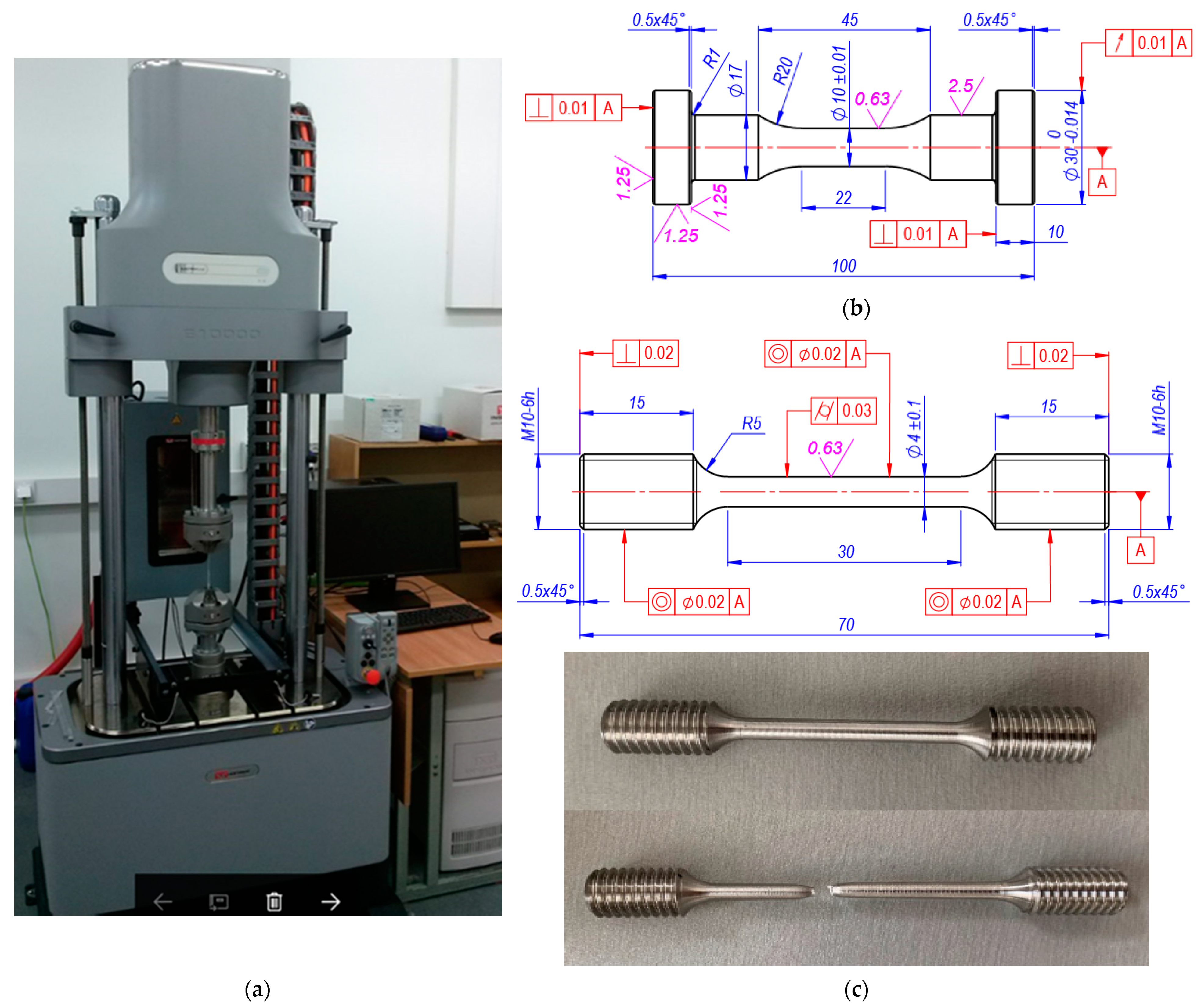
2.1. Experiment and Materials

The experimental setup consists of a 50 kN UMM-5T testing machine (Kaunas University of Technology, Kaunas, Lithuania) and an electronic part, which is designed to record stress-strain diagrams, cycles, and load reversal. A deformation rate of 4 cycles per minute was used for fatigue tests. Fatigue tests have been performed according to the GOST 25502—79 standard (Strength analysis and testing in machine building. Methods of metals mechanical testing. Methods of fatigue testing) [43]. The GOST 22015—76 standard (Quality of product, Regulation and statistical quality evaluation of metal materials and products on speed-torque characteristics) [44] was used to calculate the statistical characteristics.

Experimental monotonic tension tests were carried out with the Instron ElectroPuls E10000T (Norwood, MA, USA) series Servo Hydraulic Fatigue testing system (Figure 1a). Tensile tests have been performed according to ISO 6892-1:2016. (Metallic Materials—Tensile Testing—Part 1: Method of Test at Room Temperature; International Organization for Standardization) [45]. Mechanical characteristics were measured with an error that did not exceed ± 1% of the deformation scale.

The main task of a fatigue load device is to provide a homogeneous deformation state to the specimen to be deformed. This is achieved by the high coaxiality of the grippers and the rigidity of the machine. Samples used for cyclic deformation tests with a linear stress state must provide a homogeneous stress state in the test section of the test specimen until fatigue crack occurs. Figure 1b shows a drawing of the specimen that best satisfies these conditions.

After fatigue tests, specimens were used as workpiece materials to produce monotonous tensile specimens, with the aim of creating material properties nearly identical to those of the material subjected to cyclic loading. Monotonic tensile samples of a circular cross section with d = 4 mm and l = 30 were taken from parts of the cyclic test samples, which had not been subjected to plastic deformation (Figure 1c).

Table 1. The chemical composition of the materials.

Material	C	Si	Mn	Cr	Ni	Mo	V	S	P	Mg	Cu	Al
						%
15Cr2MoVA (GOST 5632-2014)	0.18	0.27	0.43	2.7	0.17	0.67	0.30	0.019	0.013	-	-	-
C45 (GOST 1050-2013)	0.46	0.28	0.63	0.18	0.22	-	-	0.038	0.035	-	-	-
D16T1 (GOST 4784-97)	-	-	0.70	-	-	-	-	-	-	1.6	4.5	9.32

and

Table 2. Mechanical properties of the materials.

Material	epr	σpr	σys	σu	Sk	ψ
	%		MPa			%
15Cr2MoVA (GOST 5632-2014)	0.200	280	400	580	1560	80
C45 (GOST 1050-2013)	0.260	340	340	800	1150	39
D16T1 (GOST 4784-97)	0.600	290	350	680	780	14

show the mechanical properties and chemical composition and of alloyed steel 15Cr2MoVA, structural steel C45, and aluminium alloy D16T1.

Heat resistant steel 15Cr2MoVA has been anisotropic during cyclic loading, that is, it accumulates plastic strain in the direction of tension. Structural steel C45 has been a cyclically stable anisotropic material. The D16T1 aluminium alloy has been cyclically hardened during cyclic loading with stress-limited loading and has not unilaterally accumulated plastic deformation.

Table 3. Low cycle testing programme under strain-controlled loading (${\overline{e}}_0$ = constant).

Material	$\mathbf{Loading} \mathbf{Level}, {\overline{\mathit{e}}}_0$	Number of Specimens, pcs.
15Cr2MoVA	1.8	40
	3.0	80
	5.0	40
C45	2.5	60
	4.0	100
	6.0	60
D16T1	1.0	20
	1.5	80
	2.0	20

shows the low cycle fatigue test programme. Different numbers of samples were used to determine the effect of the sample size on the statistical results.

Figure 2 shows the fatigue curves under strain-controlled loading. These curves have been developed according to the recommendations of the Regularities and Norms in Nuclear Power Engineering (PNAE) [46], which require the development of low cycle fatigue curves after a minimum of 15 specimen tests at different uniformly distributed loading levels.

In this study, three load levels were selected for low cycle fatigue testing. Reference [14] states that to obtain stable scattering of the mechanical characteristics at a single load level, 20–25 specimens should be tested. Under strain-controlled loading, the material will only fail due to fatigue, so all three loading levels have the same value. However, to investigate the effect of the batch of products on statistical performance, the number of samples was increased to 80 at the middle levels and 100 for steel C45. All test equipment’s and methods are explained in detail in the literature [47].

2.2. Review of Sensitivity Calculation Methods

Reference [15] presents the three most common methods for calculating the sensitivity threshold.

Graphical Method. The application of this method involves drawing the statistical distribution curve within the coordinates P − lgN of the probability plot under the normal distribution law. The calculations are completed when the value is characterized by straight-line positioning of the experimental points in coordinate system P – lg (N – N₀) is found. This method, however, provides only an approximate threshold sensitivity value.

Distribution Symmetry Improvement Method. Under this method, the coefficient of skewness is the key indicator of distribution symmetry:

$$S=\frac{m_3}{{\sigma }^3}$$

(1)

With normal deviation, the values of the coefficient of skewness and third central moment of distribution are equal to zero. This is the property that is employed in the search for the sensitivity threshold value. During the calculation, the sensitivity threshold N₀ value is found, the difference between the end members of rank order for random measure X″ = lg (N – N₀) is determined. The R interval is broken down into 9–15 equal parts, and the number of values is determined for each interval. Then, the values of the three initial h₁, h₂, h₃ and third central moment of distribution m₃ are determined:

$$h_1=\frac{1}{n}{\displaystyle \sum x_j{n}_j}, h_2=\frac{1}{n}{\displaystyle \sum x_j^2{n}_j}, h_3=\frac{1}{n}{\displaystyle \sum x_j^3{n}_j}.$$

(2)

$$m_3=h_3-3h_2{h}_1+2h_1^3$$

(3)

If $m_3\ne 0$, a new N₀ value is picked, and the calculations are repeated. If m₃ > 0, N₀ value is increased in the following approximation; if not—reduced. Finally, the sensitivity threshold value is selected, at which the third central moment of random value X″ = lg (N – N₀) becomes equal to zero is selected finally. To speed up the calculation process, it is recommended to create a distribution graph within coordinate system N₀ − m₃.

Least Squares Method. This method has been employed in the present paper. A random size chart, which has been distributed according to the normal law, drawn within the coordinates P − lgN of the probability plot under the normal law is presented as a straight line, the equation of which is as follows:

$$x=\overline{X}+bz$$

(4)

The distribution quantile is the value for the random normalized measure z_p corresponding by given probability measure P. Normalized random measure:

$$z_p=\frac{(x-\overline{X})}{\sigma }$$

(5)

With N₀ selected properly, the difference between the sums of mean square deviations of random measures X″ = lg (N – N₀) and the sums of mean square deviations of the random normalized measure calculated according to Formula (5) will be minimal:

$$Q={{\displaystyle \sum \left[\lg (N_i-N_0)-\overline{X}-b{z}_i\right]}}^2=Q_{\min }$$

(6)

Distribution parameters $\overline{X}$ and b are calculated based on the following equations:

$$\begin{array}{l}\frac{\delta Q}{\delta \overline{X}}=-2{\displaystyle \sum \left[\lg (N_i-N_0)-\overline{X}-b{z}_i\right]}=0,\\ \frac{\delta Q}{\delta b}=-2{\displaystyle \sum \left[\lg (N_i-N_0)-\overline{X}-b{z}_i\right]}=0,\\ \frac{\delta Q}{N_0}=-2/2.3{\displaystyle \sum \left[\frac{\lg (N_i-N_0)-\overline{X}-b{z}_i}{(N_i-N_0)}\right]}=0.\end{array}$$

(7)

In the case of the normal distribution $\sum z_i=0$. Then, measures $\overline{X}$, and b are calculated based on the first two Equation (7):

$$\overline{X}=\frac{1}{n{\displaystyle \sum \left[\lg (N_i-N_0)\right]}}$$

(8)

$$b=\frac{{\displaystyle \sum z_i}\left[\lg (N_i-N_0\right]}{{\displaystyle \sum z_i^2}}$$

(9)

Given Equations (8) and (9), measure N₀ is calculated based on the equation under the system of three Equation (7):

$${\displaystyle \sum \frac{[\lg (N_i-N_0)-1/n{\displaystyle \sum (N_i-N_0)}-z_i{\displaystyle \sum z_i\lg (N_i-N_0)/{\displaystyle \sum z_i^2}}]}{(N_i-N_0)}}=0$$

(10)

Quantile values, given probability P, are picked from the reference [15]. Event probability values are calculated using the following formula

$$P=\frac{(i-0.5)}{n}$$

(11)

2.3. Application of Sensitivity Threshold to Statistical Calculations of High-Cycle Fatigue

In the review of the results of the multicycle fatigue durability test [38] a deviation from the normal distribution has been observed with a low characteristic of the distribution of the analysed random value X′ = lgN_i has been noted. The probability of failure duration points marked in the coordinate system comprises the upward bent curves. Meanwhile, in the case of the theoretical normal distribution, the points are expected to form straight lines.

Application of new random value X″ = lg (N – N₀) to statistical calculations has led to reduction in the deviation from the theoretical normal distribution, and the experimental points in the coordinate system P – lg(N_i – N₀) have comprised straight lines. Value N₀ is referred to as the lower sensitivity threshold of the statistical distribution corresponding to the minimum number of cycles, at which the material is still likely to fail.

For statistical assessment of the high-cycle fatigue test results, it is recommended to apply the law of statistical distribution of logarithmic-normal random measure. After the sensitivity threshold has been introduced into the statistical calculations, the following changes have been observed.

• the scattering of the experimental points has been reduced;
• the statistical distribution curves have become closer to being straight;
• the coefficient of skewness has approached zero, which is characteristic of the normal and logarithmic-normal random measure distribution laws;
• the use of a small number of specimens for the tests results in the errors of calculation of the sensitivity threshold.

It has been detected [38] that in the case of high-cycle fatigue of chromium-molybdenum alloy steel, the curve for the statistical distribution of durability characteristics not only has the lower sensitivity threshold N₀, but also the upper sensitivity threshold N_k. Value N_k is usually higher than N₀ by several grades. Where random measure X″ = lg (N_i – N₀) satisfies the logarithmic-normal law of statistical distribution, and N_k is higher than N₀ by several grades, then random measure:

$$X^{‴}=\frac{N_i-N_0}{N_k-N_i}$$

(12)

Furthermore, satisfy the logarithmic-normal law described by the following expression:

$$\lg \frac{N_i-N_0}{N_k-N_i}\approx \lg (N_i-N_0)-\mathrm{constant}$$

(13)

Following insertion of random measure X‴ into the distribution function

$$F(N)=\frac{1}{\sigma \sqrt{2\pi }}{\displaystyle \underset{\infty }{\overset{\ln X^{‴}}{\int }}\exp }\left[-\frac{\ln {(X^{‴}-{\overline{X}}^{‴})}^2}{2{\sigma }^2}\right]d(\ln X^{‴})$$

(14)

Whereas the key patterns of mechanical properties are analysed as random measures, statistical distribution bounds (N₀—lower, N_k—upper) for these random values may also be determined under the maximum likelihood method. The maximum likelihood method was proposed by A. Fisher [48] and could be used to identify the lower N₀ and upper N_k—values of sensitivity thresholds.

Statistical distribution density is equal to the distribution function derivative:

$$P(N)=F^{\prime }(N)=\frac{1}{\sigma \sqrt{2\pi }}\exp \left[-\frac{\ln {(X^{‴}-{\overline{X}}^{‴})}^2}{2{\sigma }^2}\right]\times \frac{N_k-N_0}{(N_k-N_i)(N_i-N_0)}$$

(15)

With the statistical distribution values available, it is possible to build maximum likelihood function L:

$$L={\displaystyle \prod _{i=1}^{n}P(N_i)}=\frac{1}{{\sigma }^2{(2\pi )}^{\frac{n}{2}}}\times \exp \left[{\displaystyle \sum _{i=1}^n\frac{{(\ln \frac{N_i-N_0}{N_k-N_i}-{\overline{X}}^{‴})}^2}{2{\sigma }^2}}\right]\times {\displaystyle \prod _{i=1}^n\frac{N_k-N_0}{(N_k-N_i)(N_i-N_0)}}$$

(16)

The maximum likelihood function is analysed by taking its logarithm based on natural logarithm:

$$\ln L=-n\ln \sigma -\frac{n}{2}\ln 2\pi -\frac{1}{2{\sigma }^2}\times {\displaystyle \sum _{i=1}^n{\left[\ln \frac{N_i-N_0}{N_k-N_i}-{\overline{X}}^{‴}\right]}^2}+{\displaystyle \sum _{i=1}^n\ln }\frac{N_k-N_0}{(N_k-N_i)(N_i-N_0)}$$

(17)

L(x) has its maximum value within the interval, and are differentiated concerning ${\overline{X}}^{‴}$, σ, N₀, N_k then the maximum likelihood function, at its maximum point, shall be maximal L = maximum. In this case, we receive the following:

$$\frac{\delta \ln L}{\delta \overline{X}}=0, \frac{\delta \ln L}{\delta N_0}=0, \frac{\delta \ln L}{\delta \sigma }=0, \frac{\delta \ln L}{\delta N_k}=0.$$

(18)

Assessment of the maximum likelihood function is the solution of these so-called maximum likelihood equations. These equations usually have only a single solution. Differentiation of the maximum likelihood Equation (17) by ${\overline{X}}^{‴}$, σ, N₀ and N_k has resulted in four equations with four unknowns:

$$\begin{gathered} \frac{\delta \ln L}{\delta \overline{X}}=\frac{1}{{\sigma }^2}{\displaystyle \sum _{i=1}^n\left[\ln \frac{N_i-N_0}{N_k-N_i}-{\overline{X}}^{‴}\right]}=0, \\ \frac{\delta \ln L}{\delta \sigma }=-\frac{n}{\sigma }+\frac{1}{{\sigma }^3}{\displaystyle \sum _{i=1}^n\left[\ln \frac{N_i-N_0}{N_k-N_i}-{\overline{X}}^{‴}\right]}=0, \\ \frac{\delta \ln L}{\delta N_0}=\frac{1}{{\sigma }^2}{\displaystyle \sum _{i=1}^n\left\{\left[\ln \frac{N_i-N_0}{N_k-N_i}-{\overline{X}}^{‴}\right]\frac{1}{N_i-N_0}\right\}}+{\displaystyle \sum _{i=1}^n\frac{N_k-N_i}{(N_k-N_0)(N_i-N_0)}}=0, \\ \frac{\delta \ln L}{\delta N_k}=\frac{1}{{\sigma }^2}{\displaystyle \sum _{i=1}^n\left\{\left[\ln \frac{N_i-N_0}{N_k-N_i}-{\overline{X}}^{‴}\right]\frac{1}{N_k-N_i}\right\}}+{\displaystyle \sum _{i=1}^n\frac{N_0-N_i}{(N_k-N_0)(N_k-N_i)}}=0. \end{gathered}$$

(19)

In Equation (19), ${\overline{X}}^{‴}$ and σ are identified:

$${\overline{X}}^{‴}=\frac{1}{n}{\displaystyle \sum _i^n\ln \frac{N_i-N_0}{N_k-N_i}}, \sigma =\sqrt{\frac{1}{n}{\displaystyle \sum _i^n\left[\ln X^{‴}-{\overline{X}}^{‴}\right]}}.$$

(20)

Expressions ${\overline{X}}^{‴}$ and σ received are statistical estimates of the maximum likelihood function. However, they cannot be identified unless sensitivity thresholds N₀ and N_k are used. This means that the sensitivity thresholds are the key approximations of the maximum likelihood function. The Least Squares Method has been chosen for greater accuracy compared to the graphical methods; moreover, the Least Squares Method requires performing fewer calculations compared to the Distribution Symmetry Improvement Method.

2.4. Description of the Mathematical Model Function and Algorithms

For estimation of the statistical distribution sensitivity thresholds, the four Equation (19) system with four unknowns has been analysed. To identify the bottom sensitivity threshold N₀, the approximation method has been used. Whereas arithmetic mean $\overline{X}$ and average square deviation σ of the distribution function is impossible to identify unless lower N₀ and upper N_k sensitivity thresholds have been identified, the latter shall be calculated at first. The approximation method has been used only for the identification of the lower sensitivity threshold N₀ of the statistical distribution.

The large solution of Equation (19) is challenging and implies a fairly high likelihood of an error with the samples. Hence, to identify sensitivity thresholds N₀ and N_k of statistical distribution, a special algorithm has been used and a special Matlab application capable of performing the functions listed below has been designed:

• Calculation of lower sensitivity threshold N₀ of statistical distribution under approximation method following the selection of lower sensitivity threshold N_k of statistical distribution.
• Provides values of Equation (8) for possible solutions of N₀ and N_k.
• Calculates new random measure $X^{‴}=\frac{N_i-N_0}{N_k-N_i}$ for each mechanical property.
• Calculates failure probability P for each specimen.
• Calculates statistical parameters $\overline{X}$, σ, σ², S, V, and E_x of the distribution for mechanical properties of the analysed structural materials.

Initial sensitivity threshold N₀ shall not exceed the lowest value of the rank order of a mechanical property generated during the tests, and upper sensitivity threshold N_k shall not be lower than the highest value of the rank order of a mechanical property generated during the tests. If not, the calculations made by the application will fail, as random size $\ln \frac{N_i-N_0}{N_k-N_i}$, in this case, will be a logarithm of a negative number.

Under the approximation method, true sensitivity threshold N₀ is approached gradually, as lower sensitivity threshold N₀ of mechanical properties may occur in the first approximation cycle. Afterward, the calculation of Equation (19) and verification of the results obtained are provided in the algorithm. Where the resulting value is greater than or equal to zero, the verification of whether Equation (19) equals zero is performed. If so, the following equation is calculated, and the respective sensitivity thresholds are generated. In case the condition verified is not equal to zero at the initial sensitivity threshold, another approximation cycle is launched, the calculation is repeated, and verification is performed. At the increase in the lower sensitivity threshold, the interval reduces naturally, and the sought value of lower sensitivity threshold N₀ approaches the true value. When solution Equation (19) becomes negative, the MATLAB program returns to the last value of lower sensitivity threshold N₀. Further in the process of calculation, the solution of Equation (19) is found using sensitivity thresholds N₀ and N_k. Then, the condition showing that upper sensitivity threshold N_k is the final one is subject to verification. If it is not final, subsequent upper sensitivity threshold N_k is picked from array N_k, and the program is repeated from the start. If the upper sensitivity threshold N_k is final (eleventh, in this case), the calculations are completed. Then, the condition showing that upper sensitivity threshold N_k is the final one is subject to verification. If it is not final, subsequent upper sensitivity threshold N_k is picked from array N_k, and the program is repeated from the start. If the upper sensitivity threshold N_k is final (eleventh, in this case), the calculations are completed.

3. Results and Discussion

Lower N₀ and upper N_k sensitivity thresholds have been determined (

Table 4. Sensitivity thresholds for mechanical properties.

Mechanical Property	Material	N0	Nk
σpr, MPa	15Cr2MoVA C45 D16T1	184.0	410.0
		206.0	510.0
		201.8	390.0
σy, Mpa	15Cr2MoVA C45 D16T1	276.4	550.0
		206.0	510.0
		245.6	440.0
σu, Mpa	15Cr2MoVA VA 45 D16T1	445.1	700.0
		594.8	1000.0
		535.4	800.0
Sk, Mpa	15Cr2MoVA C45 D16T1	1153.5	2110.0
		874.0	1450.0
		641.7	945.0
ψ, %	15Cr2MoVA C45 D16T1	72.4	91.0
		29.2	55.0
		9.1	24.0
ψu, %	15Cr2MoVA C45 D16T1	5.8	25.3
		9.1	35.0
		10.5	15.0

) for statistical distribution under the calculation methodology discussed in the above paragraph.

Initial data for calculation of the durability of the parts and structural members operating under cyclic load or low-cycle load are the following material mechanical properties: proportionality limit σ_pr, yield strength σ_y, strength limit σ_u, failure resistance S_k, percent area reduction ψ, and percent area reduction at failure ψ_u. Scattering of mechanical properties is determined by: production process factors which determine the metal structure; specimen production process; the test method selected. In statistical investigation of the distribution of mechanical properties, the following three distribution laws are the most common: normal, logarithmic-normal, and Weibull’s. The best distribution of the sum of a fairly large number of independent random values is known to be achieved under the normal law. Hence, the normal distribution law is applied in most papers dealing with statistical investigation. To learn about the variation of statistical characteristics, in particular, the coefficient of skewness, under each distribution law by using the sensitivity threshold measure, all three distribution laws have been applied in the present paper. The following statistical characteristics have been calculated under the normal and logarithmic-normal distribution laws: arithmetic mean, mean square deviation, scattering, the third central moment, coefficient of skewness, and coefficient of variation. Under the methodology provided in reference [38], similar characteristics have been calculated for the Weibull’s distribution. These statistical characteristics have been calculated for two random measures X′ = lgX and X″ = lg(Ni – N₀). The results are provided in

Table 5. Coefficients of skewness for mechanical properties under the statistical distribution laws.

Mechanical Property	Material	Distribution Law
		Normal		Logarithmic-Normal		Weibull’s
		X′	X″	X′	X″	X′	X″
σpr, MPa	15Cr2MoVA C45 D16T1	0.07647	0.000038	−0.3199	−0.000411	0.07793	0.07793
		0.41101	0.000127	0.05815	−0.000137	0.416676	0.416682
		−0.09905	−0.000008	−0.2426	−0.000448	−0.10158	−0.010158
σy, Mpa	15Cr2MoVA C45 D16T1	0.005413	0.000003	−0.3164	−0.000427	0.005516	0.005502
		0.41101	0.000127	0.05815	−0.000137	0.416676	0.416682
		0.1197	0.000092	−0.1258	−0.000489	0.122715	0.122706
σu, Mpa	15Cr2MoVA C45 D16T1	−0.3332	−0.000166	−0.6145	−0.000658	−0.3396	−0.3396
		−0.322	−0.000099	−0.5682	−0.000316	−0.326442	−0.32643
		−0.1403	−0.000108	−0.3343	−0.000743	−0.143851	−0.143855
Sk, Mpa	15Cr2MoVA C45 D16T1	0.2425	0.000121	−0.05469	−0.000387	0.247175	0.247177
		−0.1088	−0.000034	−0.307	−0.000274	−0.110319	−0.110327
		−0.06094	−0.000047	−0.2495	−0.000671	−0.062491	−0.062505
ψ, %	15Cr2MoVA C45 D16T1	1.096878	0.000547	0.901323	−0.000013	1.436741	1.117773
		0.224567	0.000069	0.021761	−0.000081	0.227662	0.227669
		0.528782	0.000407	0.161176	−0.000074	0.542263	0.542267
ψu, %	15Cr2MoVA C45 D16T1	2.37809	0.001186	0.916574	0.000106	2.638781	2.423339
		1.445826	0.000446	0.24641	0.000011	2.219523	1.465758
		0.071902	0.000055	−0.177563	−0.000287	0.246678	0.073743

.

Analysis of the results of the calculation for the coefficient of skewness presented in Table 5 has shown that the value of the coefficient of skewness for measure X″ is considerably lower than that for measure X′. It could therefore be claimed that measure X″ is characterized by more accurate distribution under the normal law, which supports one of the expected advantages of applying the sensitivity threshold. Meanwhile, the values of the coefficients of skewness under the Weibull distribution are little different from each other and are not close to zero, which means that the Weibull’s distribution is not characteristic of random measure X′. Figure 3 and Figure 4 present the statistical distribution curves for the mechanical properties of steel 15Cr2MoVA.

A similar distribution has been observed for the mechanical properties of the other two materials. The graphic distribution view of the probability plot would suggest the following conclusions: due to greater scattering, distribution curves for random measure X″ are more sloped and differ considerably from the expected straight line. This contradicts the statement that, where the sensitivity threshold is used for statistical investigation, the statistical distribution graphs should be very close to straight lines [38]. Several patterns could be observed during the analysis of the calculated statistical properties (

Table 6. Statistical properties for mechanical properties of structural materials under the logarithmic-normal law taking into account sensitivity thresholds N₀ and N_k.

Property	Material	$\overline{\mathit{X}}$	σ	D	S	V	Ex
σpr, MPa	15Cr2MoVA	0.0145	0.4154	0.1726	−0.8310	−2.0004	1.2513
	C45	0.0109	0.4380	0.1918	−1.0160	−2.3199	1.8201
	D16T1	0.0193	0.4575	0.2093	−0.1727	−0.3776	0.2053
σy, Mpa	15Cr2MoVA	0.0169	0.4411	0.1946	0.7756	1.7582	5.0906
	C45	0.0109	0.4380	0.1918	−1.0160	−2.3199	1.8201
	D16T1	0.0199	0.4541	0.2062	0.4916	1.0824	0.6362
σu, Mpa	15Cr2MoVA	0.0165	0.4332	0.1877	1.3853	3.1976	1.7565
	C45	0.0117	0.4020	0.1616	0.0496	0.1233	0.5252
	D16T1	0.0192	0.3350	0.1122	0.2878	0.8591	4.6627
Sk, Mpa	115Cr2MoVA	0.0159	0.5068	0.2568	−0.1880	−0.3709	2.0149
	C45	0.0113	0.3651	0.1333	−0.5566	−1.5247	2.7141
	D16T1	0.0188	0.3666	0.1344	−0.2374	−0.6476	2.9361
ψ, %	15Cr2MoVA	0.0137	0.3307	0.1093	−1.1230	−3.3962	6.4751
	C45	0.0111	0.4228	0.1787	−0.7040	−1.6650	0.1065
	D16T1	0.0158	0.4902	0.2403	−1.5768	−3.2166	0.4385
ψu, %	15Cr2MoVA	0.0134	0.7288	0.5312	−1.1051	−1.5163	−0.7647
	C45	0.0081	0.7878	0.6206	−1.3378	−1.6983	−0.8945
	D16T1	0.0191	0.3477	0.1209	0.1802	0.5183	4.2422

) for the structural materials analyzed (steels 15Cr2MoVA, 45 and aluminium alloy D16T1), characterized by different cyclic properties (cyclically hardening, cyclically stable, cyclically softening). Taking into account sensitivity measures N₀ and N_k, for the statistical distribution of the mechanical properties, statistical parameters of the statistical distribution of all mechanical characteristics—statistical distribution skewness S, coefficient of variation V, as well as the kurtosis E_x—have been observed to develop fairly high values different from zero. This indicates that sensitivity thresholds N₀ and N_k affect agreement of statistical distribution to the logarithmic—normal law instead of supporting the agreement.

With measures N₀. and N_k already calculated, statistical distribution curves for all the analyzed mechanical properties (σ_pr, σ_y, σ_u, S_k, ψ, ψ_u) of the material have been developed within the coordinates $P-X^{‴}=\frac{N_i-N_0}{N_k-N_i}$. The statistical distribution curves are presented in Figure 5 and Figure 6 for steel 15Cr2MoVA, Figure 7 for steel C45 and Figure 8 for aluminum alloy D16T1.

In Figures, the statistical distribution curves have also been evaluated using 95% probability intervals (centre line indicates empirical distribution function; the right and left lines are limits of the confidence intervals).

Analysis of the nature of the statistical distribution curves has suggested that all the strength characteristics (σ_pr, σ_y, σ_u, S_k) for steel 15Cr2MoVA have demonstrated fairly satisfactory conformity to the normal distribution law, good absorption into the straight line within the mean failure probability range, and fit into the 95% probability interval (Figure 5).

Plasticity properties ψ, ψ_u of this type of steel also develop similar characteristics (Figure 6). However, they show a downward or upward bend at low and high probability values, developing the form discussed in the references. Statistical distribution curves for the mechanical properties of steel C45 have demonstrated a similar behaviour (Figure 7). They are fairly good at maintaining the sequence of strength properties (σ_pr, σ_y, σ_u, S_k). Meanwhile, they overlap in the case of steel 15Cr2MoVA.

Statistical distributions for mechanical properties of the aluminium alloy D16T1 have been demonstrating a similar behaviour to steel 15Cr2MoVA and steel C45 (Figure 8). Figure 9, Figure 10 and Figure 11 present the statistical distribution curves for the same mechanical properties (σ_pr, σ_y, σ_u, S_k) of the analysed structural material steels 15Cr2MoVA, C45, D16T without taking into account the sensitivity thresholds. These statistical distribution curves show a good approximation to the straight-line in the range of low, average, and high probabilities of strength. It could be concluded that sensitivity thresholds N₀ and N_k are not characteristic of mechanical properties. The same has been demonstrated by the statistical numeric parameters of the statistical distribution of mechanical properties (skewness S, coefficient of variation V, and kurtosis E_x).

The comparison of numeric values of the statistical parameters and characteristics of the statistical distribution curves has suggested that this is one of the reasons for the statistical curves to move considerably further from the hypothetical straight line described by the logarithmic-normal distribution law within the range of low and high probabilities.

4. Conclusions

Resulting from the statistical investigation of mechanical properties of the structural materials including the application of the maximum likelihood method to the identification of the sensitivity thresholds N₀ and N_k for the statistical distribution, the following conclusions could be drawn:

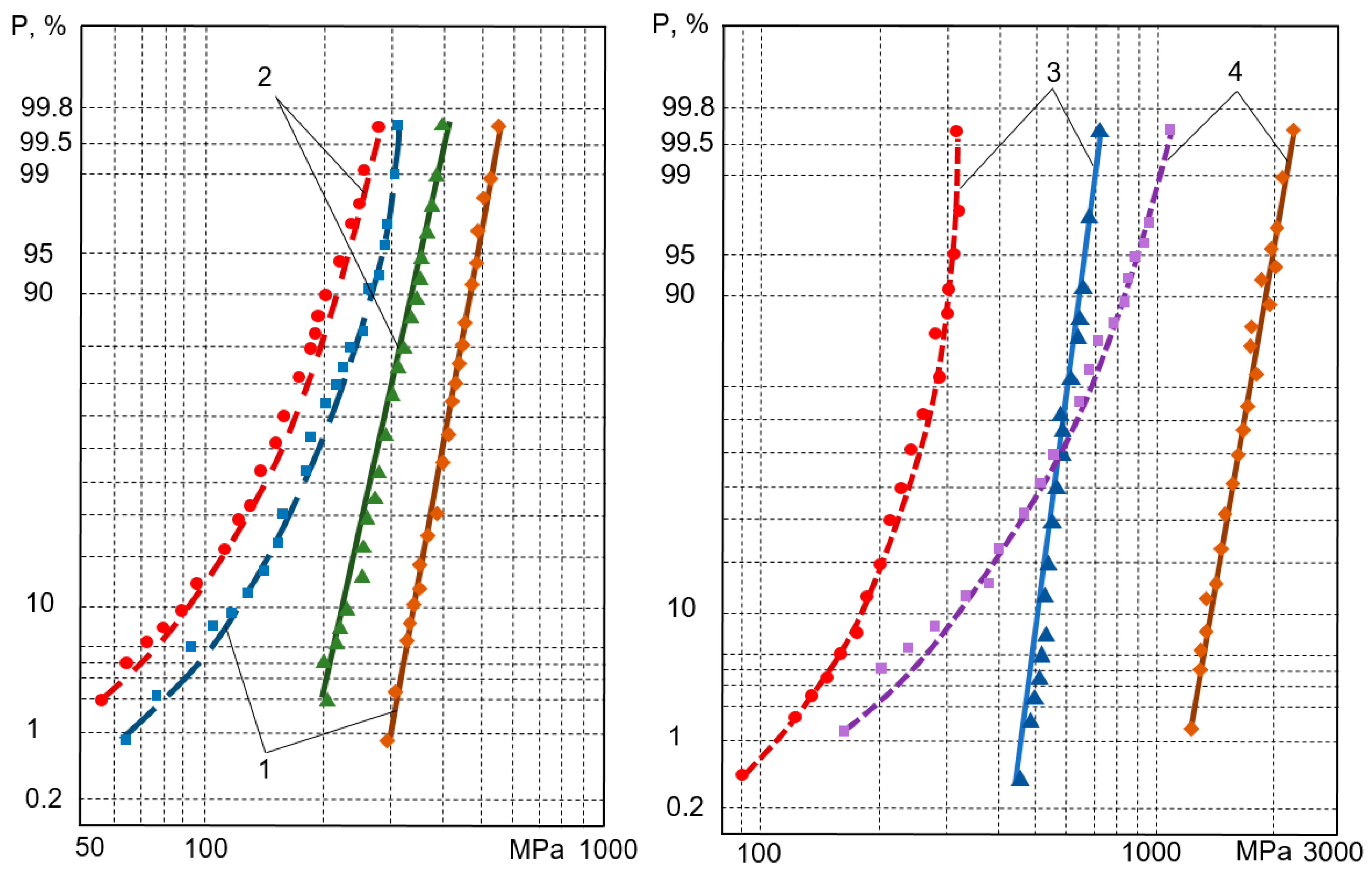
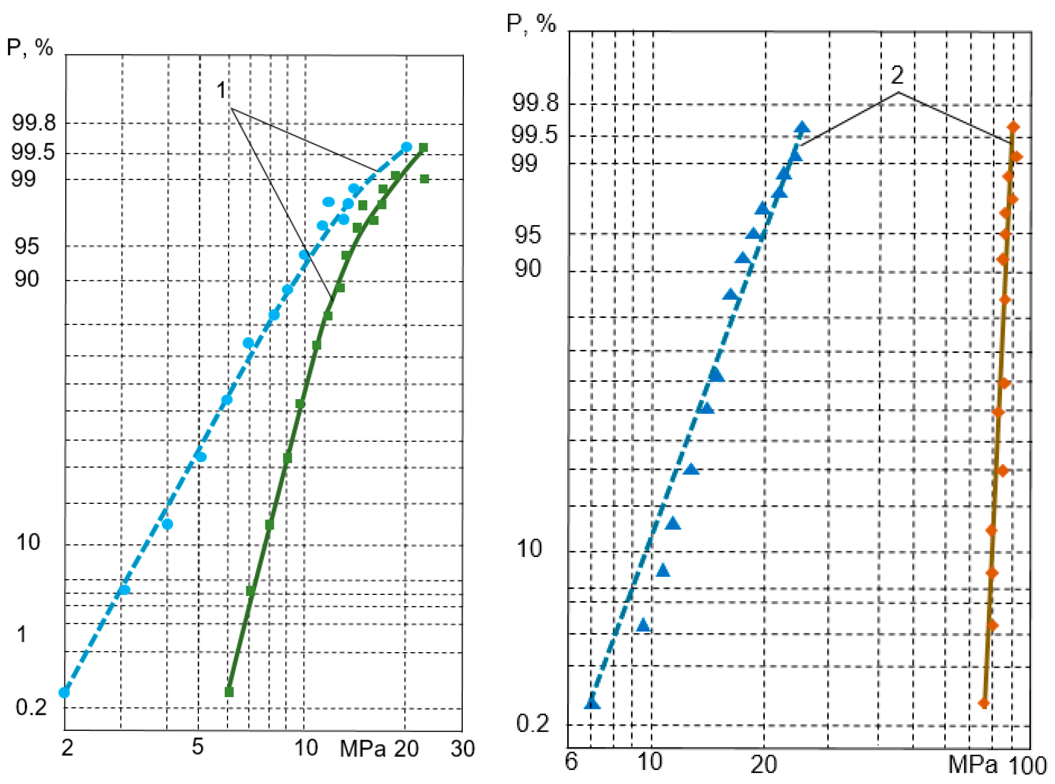
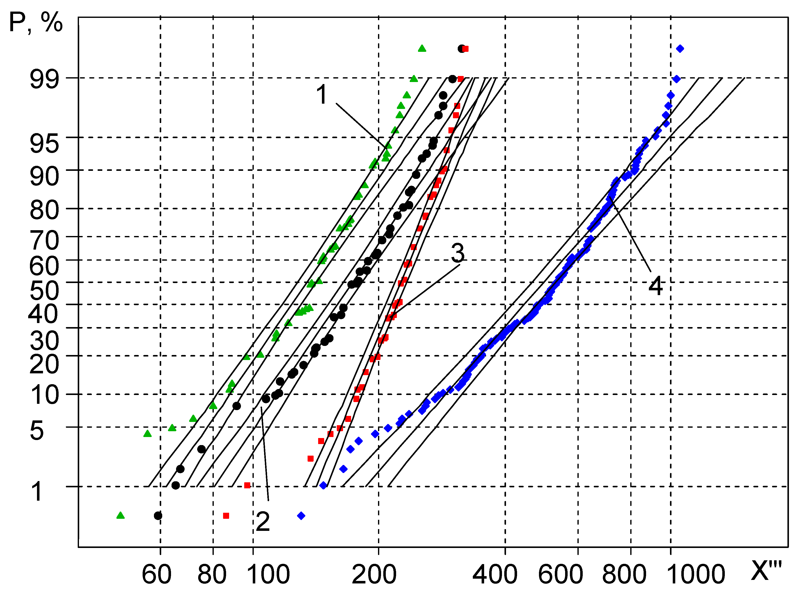
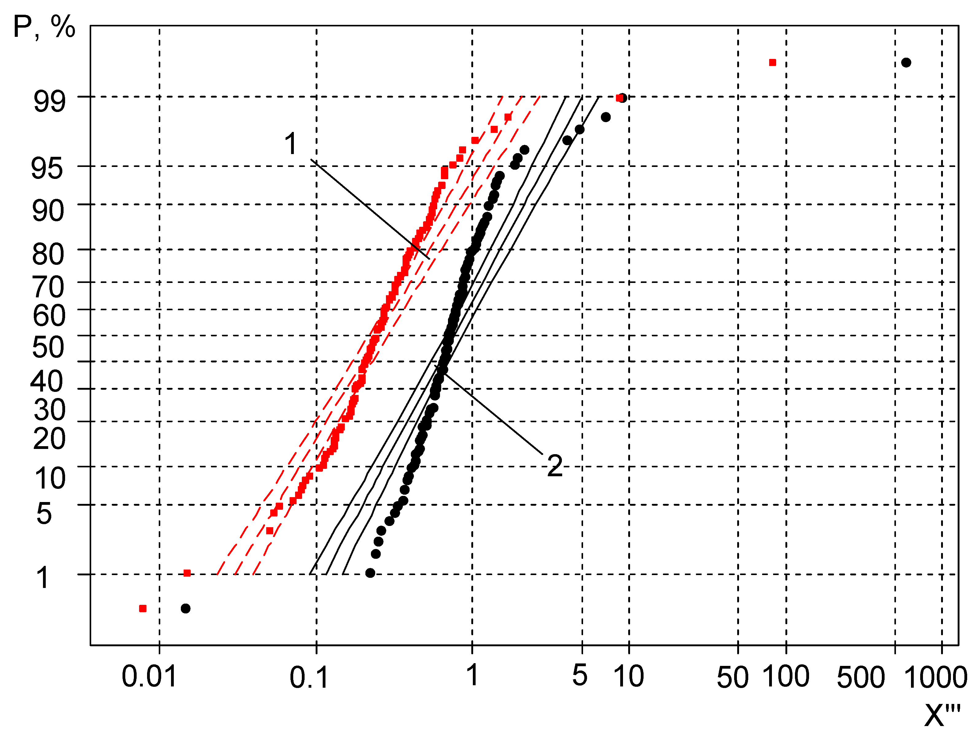
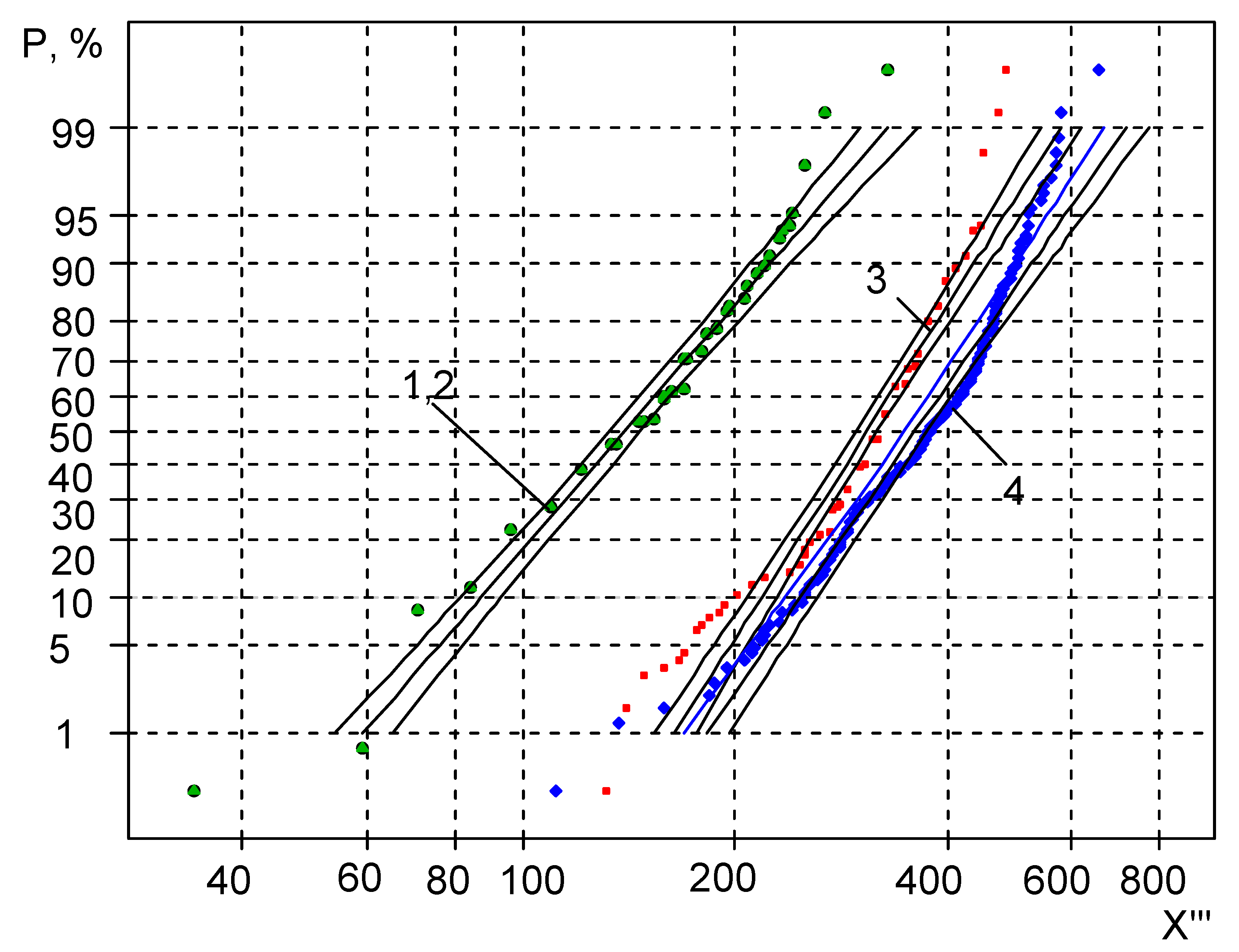
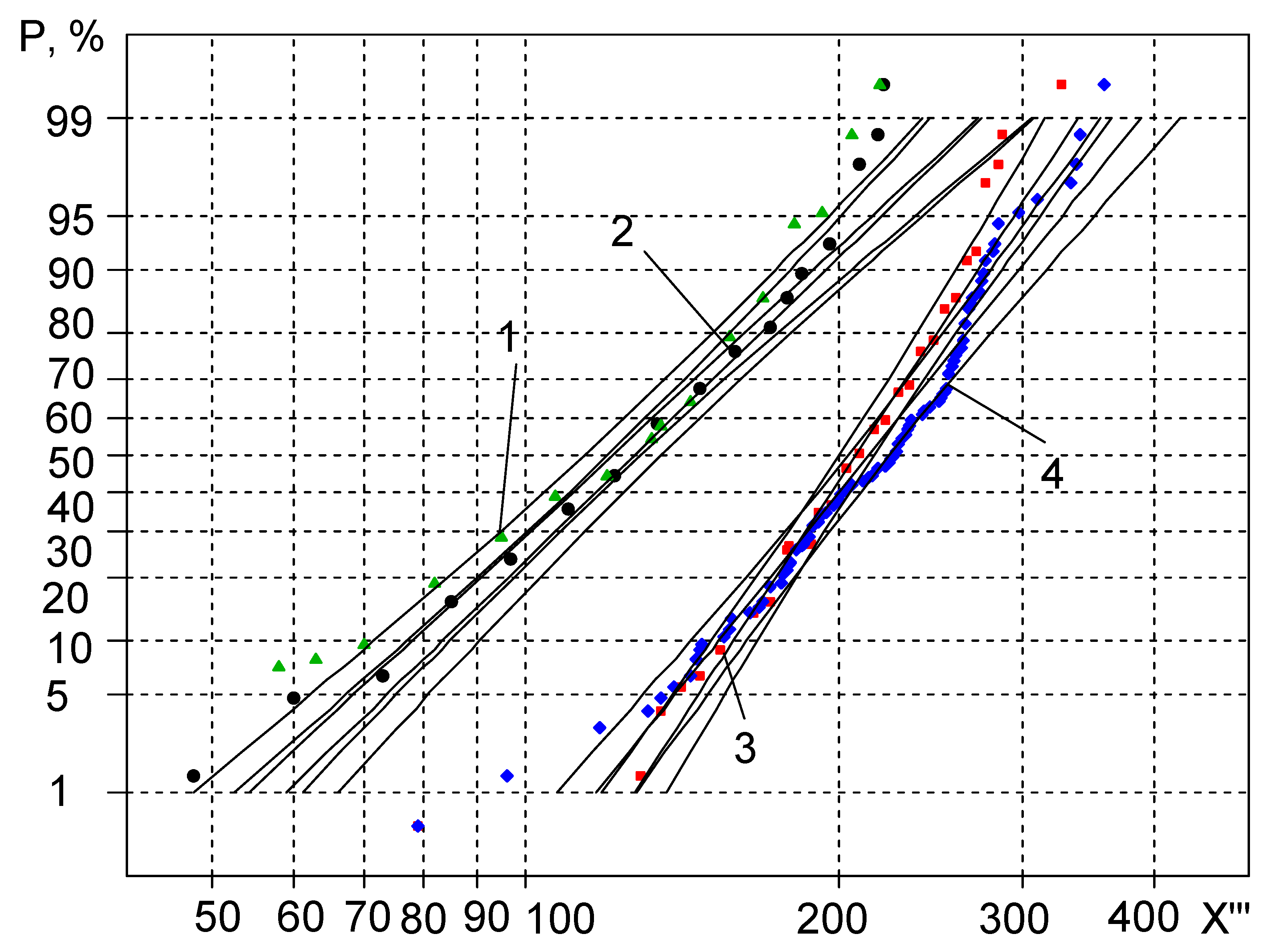
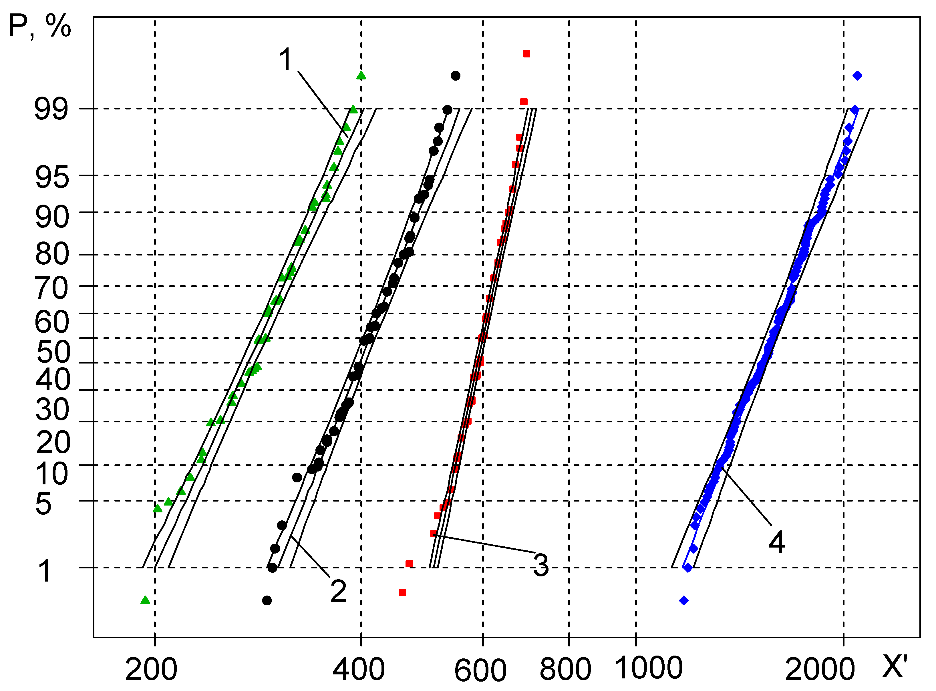
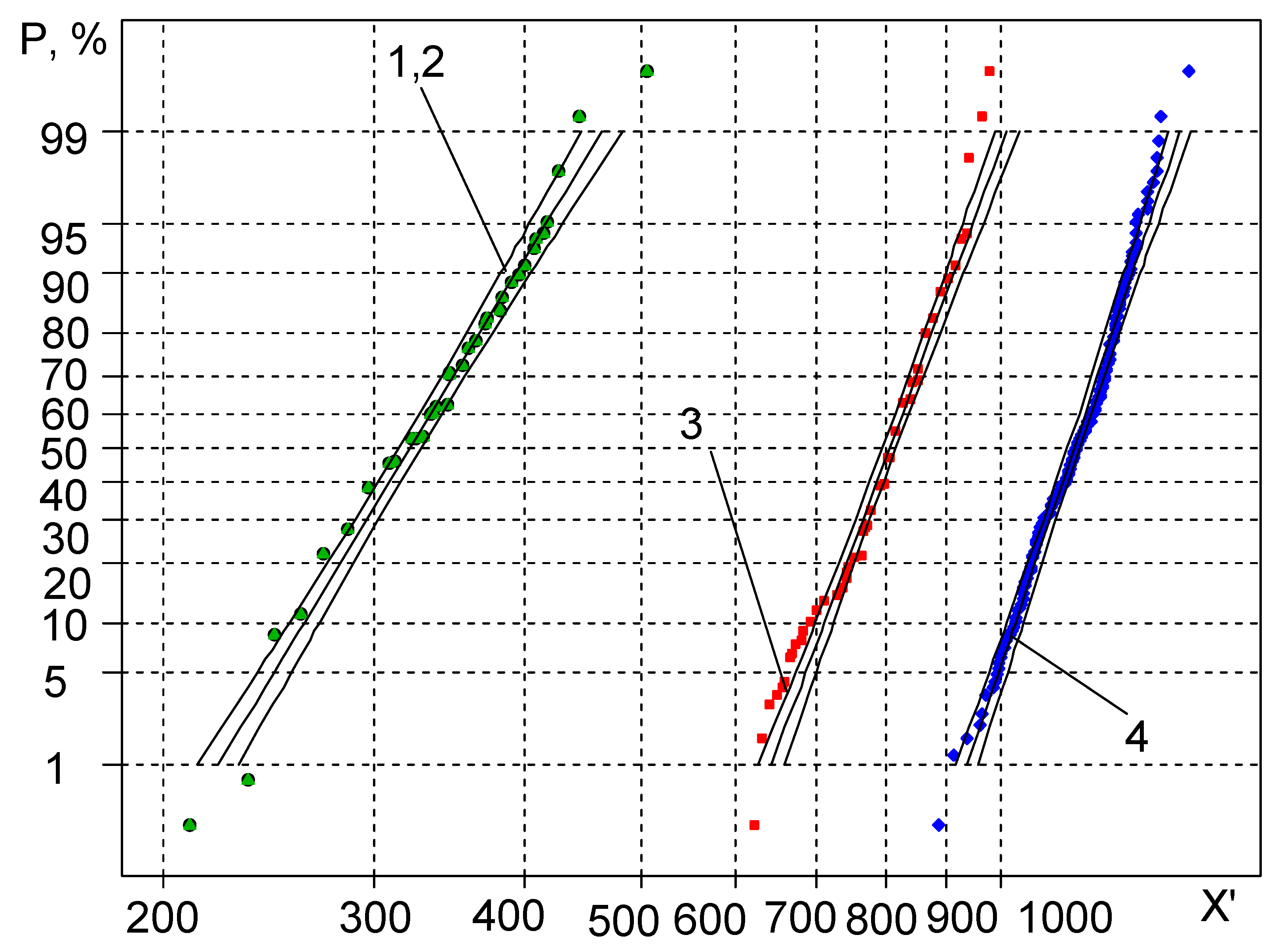
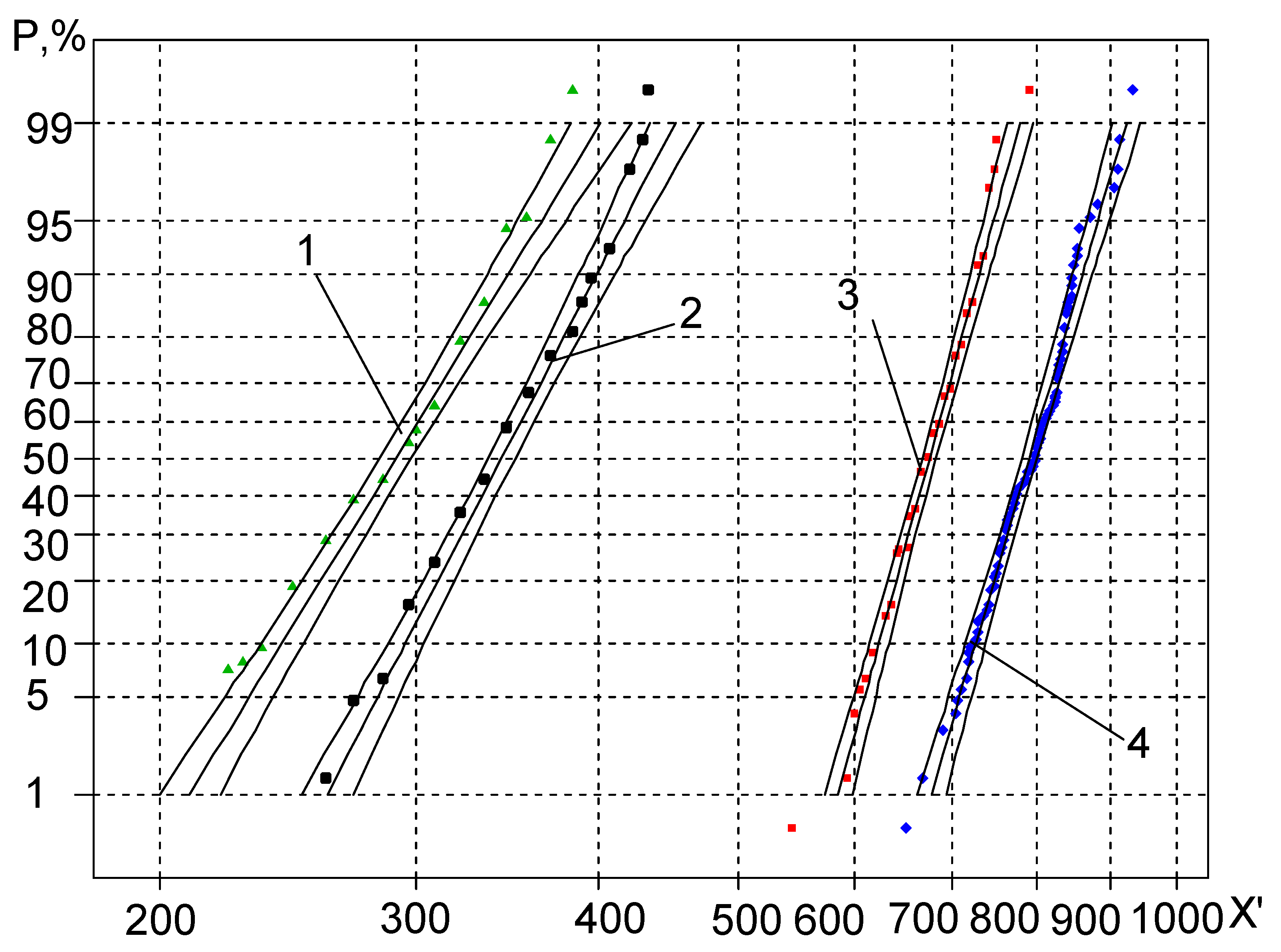
• Analysis of the graphical representation of the distribution in the probabilistic plot shows that the distribution curves for the random variable X″ are more skewed due to the higher variance. The lower part of the distribution curves for size X′ is more downward skewed. This slightly contradicts the statements in the references that, using a sensitivity threshold, the plots of the statistical distributions must be very close to straight lines. This flattening of the curves can be explained by the value of the sensitivity threshold being very close in value to the first members of the X′ variation series. As a result, the first components of X″ are closer to zero, which causes the curves to flatten.
• Application of the sensitivity threshold measure has led to decrease in the coefficient of skewness down to zero; however, the results have not corresponded to the hypothetical straight-line, unlike expected. This demonstrates that, application of the sensitivity threshold would be unreasonable.
• In the calculation of the statistical characteristics of the Weibull distribution, the coefficient of skewness S_k for the variable measures X′ and X″, the difference between the values is small. This suggests that the Weibull’s distribution is not characteristic of measure X′.
• The minimum number of elements of rank order, which still allows a reliable calculation of the sensitivity threshold measure N₀, was different for each material and did not depend directly on the initial number of elements.
• Sensitivity thresholds N₀ and N_k cannot be used for the description of the statistical distribution of mechanical characteristics skewness, coefficient of variation, and kurtosis develop values that are fairly distant from zero, supporting the fact that the statistical distribution moves further from the norm rather than approximating it.
• During analysis of the statistical distribution curves for mechanical properties, it has been observed that the application of sensitivity thresholds N₀ and N_k within the ranges of the average probabilities of statistical distribution has led to a fairly good straight line approximation of the curves, while the curves tend to bend downward and upward in the case of low and high probability values and develop the primal form.
• The estimated values of the random variable X‴ (the approximate part of the straight line) belong to the range of 40–60% probability values, allowing 50% acceptance probability values of the random variables to perform further low cycle fatigue calculations.

References

1. Makhutov, N.A. Structural Durability, Resource and Tech. Safety; Nauka: Novosibirsk, Russia, 2005; Volume 1. (In Russian) [Google Scholar]
2. Makhutov, N.A. Structural Durability, Resource and Tech. Safety; Nauka: Novosibirsk, Russia, 2005; Volume 2. (In Russian) [Google Scholar]
3. Zhu, S.-P.; Huang, H.-Z.; Smith, R.; Ontiveros, V.; He, L.-P.; Modarres, M. Bayesian framework for probabilistic low cycle fatigue life prediction and uncertainty modeling of aircraft turbine disk alloys. Probabilistic Eng. Mech. 2013, 34, 114–122. [Google Scholar] [CrossRef]
4. Zhu, S.-P.; Huang, H.-Z.; Peng, W.; Wang, H.-K.; Mahadevan, S. Probabilistic physics of failure-based framework for fatigue life prediction of aircraft gas turbine discs under uncertainty. Reliab. Eng. Syst. Saf. 2016, 146, 1–12. [Google Scholar] [CrossRef]
5. Heyraud, H.; Robert, C.; Mareau, C.; Bellett, D.; Morel, F.; Belhomme, N.; Dore, O. A two-scale finite element model for the fatigue design of large welded structures. Eng. Fail. Anal. 2021, 124, 105280. [Google Scholar] [CrossRef]
6. Burger, M.; Dreßler, K.; Speckert, M. Load assumption process for durability design using new data sources and data analytics. Int. J. Fatigue 2021, 145, 106116. [Google Scholar] [CrossRef]
7. Gadolina, I.V.; Makhutov, N.A.; Erpalov, A.V. Varied approaches to loading assessment in fatigue studies. Int. J. Fatigue 2021, 144, 106035. [Google Scholar] [CrossRef] [PubMed]
8. Weibull, W. Fatigue Testing and Analysis of Results; Pergamon Press: New York, NY, USA, 1961; Available online: https://books.google.lt/books?hl=lt&lr=&id=YM4gBQAAQBAJ&oi=fnd&pg=PP1&dq=Weibull,+W.+Fatigue+Testing+and+Analysis+of+Results&ots=VIVGA6VzJY&sig=UsrDkGvsP8go6hPS6IuYK3q9-H0&redir_esc=y#v=onepage&q=Weibull%2C%20W.%20Fatigue%20Testing%20and%20Analysis%20of%20Results&f=false (accessed on 20 December 2021).
9. Weibull, W.; Rockey, K.C. Fatigue Testing and Analysis of Results. J. Appl. Mech. 1962, 29, 607. [Google Scholar] [CrossRef]
10. Freudenthal, A.M.; Gumbel, E.J. On the statistical interpretation of fatigue tests. Proc. R. Soc. Lond. Ser. A 1953, 216, 309–332. [Google Scholar] [CrossRef]
11. Freudenthal, A.M.; Gumbel, E.J. Physical and Statistical Aspects of Fatigue. Adv. Appl. Mech. 1956, 4, 117–158. [Google Scholar] [CrossRef]
12. Iida, K.; Inoue, H. Evaluation of low cycle fatigue design curve based on life distribution shape. J. Soc. Nav. Archit. Jpn. 1973, 133, 235–247. [Google Scholar] [CrossRef]
13. Serensen, S.V.; Shneiderovich, R.M. Deformations and rupture criteria under low-cycles fatigue. Exp. Mech. 1966, 6, 587–592. [Google Scholar] [CrossRef]
14. Serensen, S.V.; Kogayev, V.P.; Shneiderovich, R.M. Load Carrying Ability and Strength Evaluation of Machine Components, 3rd ed.; Mashinostroeniya: Moscow, Russia, 1975; pp. 255–311. (In Russian) [Google Scholar]
15. Stepnov, M.N. Statistical Methods for Computation of the Results of Mechanical Experiments, Mechanical Engineering; Mashinostroeniya: Moscow, Russia, 2005. (In Russian) [Google Scholar]
16. Jiang, Z.; Han, Z.; Li, M. A probabilistic model for low-cycle fatigue crack initiation under variable load cycles. Int. J. Fatigue 2022, 155, 106528. [Google Scholar] [CrossRef]
17. Makhutov, N.A.; Panov, A.N.; Yudina, O.N. The development of models of risk assessment complex transport systems. In Proceedings of the IOP Conference Series: Materials Science and Engineering, Proceedings of the V International Scientific Conference, Survivability and Structural Material Science (SSMS 2020), Moscow, Russia, 27–29 October 2020; Institute of Physics Publishing (IOP): Moscow, Russia, 2020; Volume 1023. Available online: https://scholar.google.lt/scholar?hl=lt&as_sdt=0%2C5&q=The+development+of+models+of+risk+assessment+complex+transport+systems&btnG= (accessed on 22 December 2021).
18. Tomaszewski, T.; Strzelecki, P.; Mazurkiewicz, A.; Musiał, J. Probabilistic estimation of fatigue strength for axial and bending loading in high-cycle fatigue. Materials 2020, 13, 1148. [Google Scholar] [CrossRef] [PubMed] [Green Version]
19. Li, X.-K.; Chen, S.; Zhu, S.-P.; Ding Liao, D.; Gao, J.-W. Probabilistic fatigue life prediction of notched components using strain energy density approach. Eng. Fail. Anal. 2021, 124, 105375. [Google Scholar] [CrossRef]
20. Strzelecki, P. Determination of fatigue life for low probability of failure for different stress levels using 3-parameter Weibull distribution. Int. J. Fatigue 2021, 145, 106080. [Google Scholar] [CrossRef]
21. Correia, J.; Apetre, N.; Arcari, A.; Jesus, A.D.; Muñiz-Calvente, M.; Calçada, R.; Berto, F.; Fernández-Canteli, A. Generalized probabilistic model allowing for various fatigue damage variables. Int. J. Fatigue 2017, 100, 187–194. [Google Scholar] [CrossRef]
22. Angulo, S.C.; Silva, N.V.; Lange, D.A.; Tavares, L.M. Probability distributions of mechanical properties of natural aggregates using a simple method. Constr. Build. Mater. 2020, 233, 117269. [Google Scholar] [CrossRef]
23. Matvienko, Y.G.; Kuzmin, D.A.; Reznikov, D.O.; Potapov, V.V. Assessment of the Probability of Fatigue Fracture of Structural Components with Accounting for the Statistical Scatter of Mechanical Properties of the Material and the Residual Defectness. J. Mach. Manuf. Reliab. 2021, 50, 302–311. [Google Scholar] [CrossRef]
24. Guo, S.; Liu, R.; Jiang, X.; Zhang, H.; Zhang, D.; Wang, J.; Pan, F. Statistical Analysis on the Mechanical Properties of Magnesium Alloys. Materials 2017, 10, 1271. [Google Scholar] [CrossRef] [PubMed] [Green Version]
25. Skejić, D.; Dokšanović, T.; Čudina, I.; Mazzolani, F.M. The Basis for Reliability-Based Mechanical Properties of Structural Aluminium Alloys. Appl. Sci. 2021, 11, 4485. [Google Scholar] [CrossRef]
26. Armentani, E.; Greco, A.; De Luca, A.; Sepe, R. Probabilistic Analysis of Fatigue Behavior of Single Lap Riveted Joints. Appl. Sci. 2020, 10, 3379. [Google Scholar] [CrossRef]
27. Narayanan, G. Probabilistic fatigue model for cast alloys of aero engine applications. Int. J. Struct. Integr. 2021, 12, 454–469. [Google Scholar] [CrossRef]
28. Makhutov, N.A.; Zatsarinny, V.V.; Reznikov, D.O. Fatigue prediction on the basis of analysis of probabilistic mechanical properties. AIP Conf. Proc. 2020, 2315, 40025. [Google Scholar] [CrossRef]
29. Daunys, M.; Šniuolis, R. Statistical evaluation of low cycle loading curves parameters for structural materials by mechanical characteristics. Nucl. Eng. Des. 2006, 236, 13. [Google Scholar] [CrossRef]
30. Daunys, M.; Šniuolis, R.; Stulpinaite, A. Evaluation of cyclic instability by mechanical properties for structural materials. Mechanics 2012, 18, 280–284. [Google Scholar] [CrossRef] [Green Version]
31. Raslavičius, L.; Bazaras, Ž.; Lukoševičius, V.; Vilkauskas, A.; Česnavičius, R. Statistical investigation of the weld joint efficiencies in the repaired WWER pressure vessel. Int. J. Press. Vessel. Pip. 2021, 189, 104271. [Google Scholar] [CrossRef]
32. Bazaras, Z. Analysis of probabilistic low cycle fatigue design curves at strain cycling. Indian J. Eng. Mater. Sci. 2005, 12, 411–418. Available online: https://scholar.google.lt/scholar?hl=lt&as_sdt=0%2C5&q=Bazaras%2C+Z.+2005.+Analysis+of+probabilistic+low+cycle+fatigue+design+curves+at+strain+cycling%2C+Indian+Journal+of+Engineering+%26+Material+Sciences+2%3A+411-418.&btnG= (accessed on 22 December 2021).
33. Daunys, M.; Bazaras, Z.; Timofeev, B.T. Low cycle fatigue of materials in nuclear industry. Mechanics 2008, 73, 12–17. Available online: https://scholar.google.lt/scholar?hl=lt&as_sdt=0%2C5&q=28.%09Daunys%2C+M.%3B+Bazaras%2C+Z.%3B+Timofeev%2C+B.+T.+Low+cycle+fatigue+of+materials+in+nuclear+industry&btnG= (accessed on 22 December 2021).
34. Giannella, V. Stochastic approach to fatigue crack-growth simulation for a railway axle under input data variability. Int. J. Fatigue 2021, 144, 106044. [Google Scholar] [CrossRef]
35. Giannella, V.; Sepe, R.; Borrelli, A.; De Michele, G.; Armentani, E. Numerical investigation on the fracture failure of a railway axle. Eng. Fail. Anal. 2021, 129, 105680. [Google Scholar] [CrossRef]
36. Giannella, V.; Perrella, M.; Citarella, R. Efficient FEM-DBEM coupled approach for crack propagation simulations. Theor. Appl. Fract. Mech. 2017, 91, 76–85. [Google Scholar] [CrossRef]
37. Salari, M. Fatigue crack growth reliability analysis under random loading. Int. J. Struct. Integr. 2020, 11, 157–168. [Google Scholar] [CrossRef]
38. Stepnov, M.N.; Giacintov, E.V. Fatigue of Light Structural Alloys; Mashinostroeniya: Moscow, Russia, 1973; pp. 8–22. (In Russian) [Google Scholar]
39. Ulbrich, D.; Selech, J.; Kowalczyk, J.; Jóźwiak, J.; Durczak, K.; Gil, L.; Pieniak, D.; Paczkowska, M.; Przystupa, K. Reliability Analysis for Unrepairable Automotive Components. Materials 2021, 14, 7014. [Google Scholar] [CrossRef] [PubMed]
40. Żurek, J.; Małachowski, J.; Ziółkowski, J.; Szkutnik-Rogoż, J. Reliability Analysis of Technical Means of Transport. Appl. Sci. 2020, 10, 3016. [Google Scholar] [CrossRef]
41. Ballo, F.; Comolli, F.; Gobbi, M.; Mastinu, G. Motorcycle Structural Fatigue Monitoring Using Smart Wheels. Vehicles 2020, 2, 648–674. [Google Scholar] [CrossRef]
42. Lukoševičius, V.; Makaras, R.; Rutka, A.; Keršys, R.; Dargužis, A.; Skvireckas, R. Investigation of Vehicle Stability with Consideration of Suspension Performance. Appl. Sci. 2021, 11, 9778. [Google Scholar] [CrossRef]
43. GOST 25502-79 Standard; Strength Analysis and Testing in Machine Building. Methods of Metals Mechanical Testing. Methods of Fatigue Testing; Standardinform: Moscow, Russia, 1993.
44. GOST 22015-76 Standard; Quality of Product. Regulation and Statistical Quality Evaluation of Metal. Materials and Products on Speed-torque Characteristics; Standardinform: Moscow, Russia, 2010.
45. EN ISO 6892-1:2016; Metallic Materials—Tensile Testing—Part. 1: Method of Test. at Room Temperature; International Organization for Standardization (ISO): Geneva, Switzerland, 2016.
46. Regularities and Norms in Nuclear Power Engineering (PNAE) No. G-7-002-89; Rules of Equipment and Pipelines Strength Calculation of Nuclear Power Plant; Energoatomizdat: Moscow, Russia, 1989.
47. Daunys, M. Cycle Strength and Durability of Structures; Technologija: Kaunas, Lithuania, 2005. (In Lithuanian) [Google Scholar]
48. Severini, T.A. Likelihood Methods in Statistics; Oxford University Press: Oxford, UK, 2001. [Google Scholar]
Figure 1. Equipment for tensile testing experiment (a), shape and dimension of the specimens for: (b) low—cycle fatigue tension-compression experiments, (c) monotonous tensile experiments (Units in mm).
Metals 12 00175 g001
Figure 2. Low cycle fatigue durability curves under strain-controlled loading: 1—aluminium alloy D16T, 2—alloyed steel 15Cr2MoVA, 3—structural steel C45.
Metals 12 00175 g002
Figure 3. Statistical distribution curves for mechanical properties of steel 15Cr2MoVA: random value X′ (straight lines) and random value X″ (dashed lines); 1—σy, 2—σpr, 3—σu, 4—Sk.
Metals 12 00175 g003
Figure 4. Statistical distribution curves for mechanical properties of steel 15Cr2MoVA: random value X′ (straight lines) and random value X″ (dashed lines); 1—ψ, 2—ψu.
Metals 12 00175 g004
Figure 5. Statistical distribution curves for the mechanical properties of steel 15Cr2MoVA with identified sensitivity thresholds N0 and Nk (1—σy, 2—σpr, 3—σu, 4—Sk).
Metals 12 00175 g005
Figure 6. Statistical distribution curves for the mechanical properties of steel 15Cr2MoVA with identified sensitivity thresholds N0 and Nk (1—ψ, 2—ψu).
Metals 12 00175 g006
Figure 7. Statistical distribution curves for the mechanical properties of steel C45 with identified sensitivity thresholds N0 and Nk (1—σy, 2—σpr, 3—σu, 4—Sk).
Metals 12 00175 g007
Figure 8. Statistical distribution curves for the mechanical properties of steel D16T with identified sensitivity thresholds N0 and Nk (1—σy, 2—σpr, 3—σu, 4—Sk).
Metals 12 00175 g008
Figure 9. Statistical distribution curves for the mechanical properties of steel 15Cr2MoVA without adjusting for the sensitivity thresholds N0 and Nk (1—σy, 2—σpr, 3—σu, 4—Sk).
Metals 12 00175 g009
Figure 10. Statistical distribution curves for the mechanical properties of steel C45 without adjusting for the sensitivity thresholds N0 and Nk (1—σy, 2—σpr, 3—σu, 4—Sk).
Metals 12 00175 g010
Figure 11. Statistical distribution curves for the mechanical properties of steel D16T without adjusting for the sensitivity thresholds N0 and Nk (1—σy, 2—σpr, 3—σu, 4—Sk).
Metals 12 00175 g011