A 3D Polycrystalline Plasticity Model for Isotropic Linear Evolution of Intragranular Misorientation with Mesoscopic Plastic Strain in Stretched or Cyclically Deformed Metals

Abstract

Two-dimensional electron back-scattered diffraction (2D-EBSD) mapping has been widely used for indicating the polycrystalline plasticity through intragranular misorientation parameters KAM and GROD, based on the empirically linear relationship between their average values and the mesoscopic plastic strain, in both stretched and cyclically deformed metals. However, whether the intragranular misorientation measured on the 2D-EBSD observational plane objectively reflects the 3D polycrystalline plasticity or not is a rarely reported issue. In this research, we firstly compared the KAM and GROD values measured on 2D-EBSD observational planes with different angles to loading axis of a specimen in both undeformed clamp sections and deformed gauge section, to verify whether their average values increase isotropically or not with mesoscopic plastic strain. Then, we proposed six fundamental assumptions and developed a modified 3D polycrystalline plasticity model based on the 2D polycrystalline plasticity model in our previous work. This 3D polycrystalline plasticity model can explain the isotropic linear evolution of intragranular misorientation in deformed low alloy steel with uniform equiaxial grains.

1. Introduction

Two-dimensional (2D) electron back-scattered diffraction (EBSD) mapping is now a standard analysis on intragranular misorientation in both stretched and cyclically deformed metals, whose contrast can further indicate the mesoscopic plastic strain distribution [1] through intragranular misorientation parameters such as Kernel Averaged Misorientation (KAM) and Grain Reference Orientation Deviation (GROD) firstly proposed by Wright, S.I. et al. [2,3]. KAM is typically defined as the averaged misorientation between a kernel point and its surrounding points excluding those out of grain boundary, which is also called “Local Misorientation (M_L)” by Kamaya, M. [4]. GROD is typically defined as the misorientation between an individual point and the intragranular reference point, whose average value is also called “Crystal Deformation (C_d)” or “Modified Crystal Deformation (MCD)” by Kamaya, M. [5,6]. Their capability of indicating mesoscopic plastic strain is based on the following experimental phenomenon: both $\overline{KAM}$ (M_ave) and $\overline{GROD}$ (C_d, MCD) averaged over multiple grains always linearly increase with the tensile strain ${\epsilon }^{\mathrm{T}}$ or cyclic strain upper ${\epsilon }_{\max }^{\mathrm{C}}$ applied in specimens according to abundant EBSD observation results reported in Refs. [4,5,6,7,8,9], as shown in Figure 1. To this end, average $\overline{KAM}$ and $\overline{GROD}$ have been widely used for identifying the fracture modes [10,11,12,13,14], evaluating the fatigue [15,16,17] and creep [18,19,20] damage degree, analyzing the grain boundary induced micro-cracking [21] or fretting contact-induced micro-cracking [22], and predicting the fatigue crack tip growth rate da/dN [23] or driving force ∆K [9] as two important mesoscopic plasticity indicators.

The linear evolution of average $\overline{KAM}$ and $\overline{GROD}$ with mesoscopic plastic strain was only reported by the above literature [4,5,6,7,8,9] as a common phenomenon in polycrystalline metals without providing any physical model explanations, which weakens its reliability in the industry application. According to the mainstream view represented by Wilkinson, A.J. [24,25,26,27,28,29], Kysar, J.W. [30,31,32,33,34,35], Pantleon, W. [36] and Raabe, D. [37,38] et al., KAM is regarded as an EBSD-based metric approximately measuring a special category of intragranular dislocations termed “geometrically necessary dislocation” [39,40], which can be derived from the continuum dislocation theory established by Nye, J.F. [41], Bilby, B.A. [42] and Kroner, E. [43]. However, the local geometrically necessary dislocation density cannot be linearly linked to the mesoscopic plastic strain, although it has a positive correlation with the plastic deformation in most cases. Harte, A. et al. [44] compared intragranular misorientation and plastic strain on the surface of a deformed Ni-based superalloy and revealed that the above linear relationship only works between the average misorientation and mean grain distortion in a statistical sense, while the local misorientation is the result of the number, strength and spatial distribution of intragranular slip modes and their interactions with microstructural features such as grain boundaries.

At the same time, the selection of a 2D-EBSD observational plane relative to the three-dimensional (3D) mesoscopic stress/strain principal axes is also a potential factor which may influence the $\overline{KAM}$ and $\overline{GROD}$ values. In other words, whether the linear evolution of average $\overline{KAM}$ and $\overline{GROD}$ with plastic strain reported in the above literature has the nature of isotropy or not is also an important issue to be clarified for polycrystalline metals with uniform equiaxial grains, which was rarely investigated currently. In our previous work [45], a 2D polycrystalline plasticity model considering the grain boundaries’ constraint effect on intragranular lattice rotation was established. However, the above 2D polycrystalline plasticity model has not yet been generalized to the 3D case. To address the above issues, both experimental and theoretical work was carried out in this research.

On one hand, mechanical tests on low alloy steel with uniform equiaxial grains were carried out by standard round bar specimens in this research at first, and then followed by 2D-EBSD observations on those deformed or undeformed sections. Since the linear evolution law of average $\overline{KAM}$ and $\overline{GROD}$ has been confirmed by many studies [4,5,6,7,8,9], we mainly focused on comparing the $\overline{KAM}$ and $\overline{GROD}$ values measured on 2D-EBSD observational planes with different angles to loading axis in the same specimen, to verify whether they increase isotropically or not with the mesoscopic plastic strain. The isotropic evolution law is very important for averaged $\overline{KAM}$ and $\overline{GROD}$ because these parameters can serve as the objective plasticity indicators in actual applications only if their values are independent of the observation, including the selection of 2D-EBSD observational planes.

On the other hand, a 3D polycrystalline plasticity model was established based on six fundamental assumptions to explain the linear evolution law of averaged $\overline{KAM}$ and $\overline{GROD}$ reported by other studies [4,5,6,7,8,9], as well as their isotropic evolution law observed in this research. The polycrystalline plasticity model contains two scale levels: mesoscopic scale and microscopic scale. It is assumed that the Representative Volume Element (RVE, contains multiple grains) in the mesoscopic scale is homogeneous isotropic and follows the classical J₂ finite strain plasticity theory [46], while each grain in the microscopic scale follows the crystal plasticity theory. Several necessary simplifications, such as spherical grain hypothesis and minimum activated slip factors number hypothesis, were made in the above assumptions to make the mathematical derivation of $\overline{KAM}$ and $\overline{GROD}$ evolution easier.

2. Materials and Methods

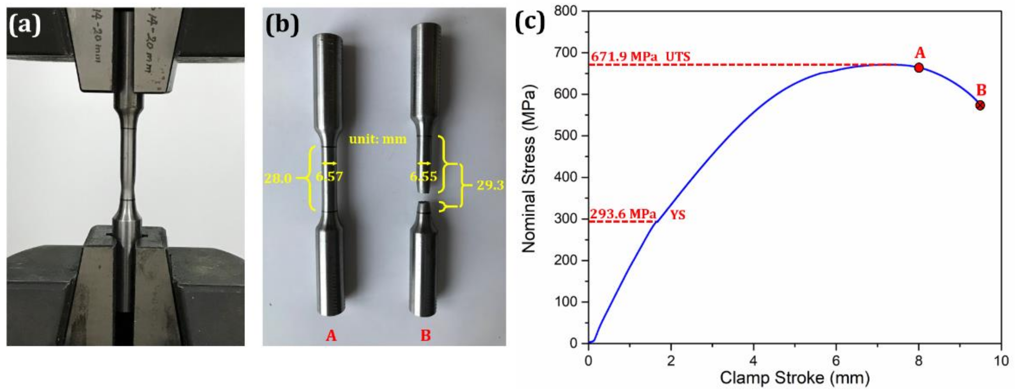
2.1. Material and Mechanical Tests

The material used in this research is type 40Cr low alloy steel in Chinese Brand, whose chemical elements and mechanical properties are shown in

Table 1. Chemical elements and mechanical properties of type 40Cr low alloy steel.

Chemical Elements (wt.%)	C	Cr	Si	Mn
	0.36%	1.56%	0.41%	1.27%
Mechanical Properties	Yield Strength (YS)		Ultimate Tensile Strength (UTS)
	293.6 MPa		671.9 MPa

. The samples for tensile mechanical tests were cut from a hot rolled plate. For higher resolution under EBSD observation, it was annealed at 850 °C for about 120 min, and followed by furnace cooling. The microstructures after heat treatment are uniform equiaxial grains made up of Body-Centered Cubic (BCC) ferrite and pearlite phases, and no initial texture exists before the plastic deformation. The metallographic figure and Inverse Pole Figure (IPF) can be referred to Ref. [9], belonging to our previous work using the same material.

The mechanical tests were carried out by two round bar specimens in type WDW-100^® machine (Instron Inc., Norwood, MA, USA) at room temperature based on ASTM E8-08 [47] standard as shown in Figure 2a, and the loading speed for tension was set as 0.5 mm/min (statically loading). The diameters of gauge section and clamp section of round bar specimen are 7 and 14 mm, respectively, while the initial gauge length and clamp length are 25 mm and 38 mm respectively. Specimen B was continually elongated until rupture to give the full nominal stress–clamp stroke curve, while Specimen A was interrupted at nominal stress of 664.6 MPa before the obvious necking behavior appears for the following EBSD observation and analysis, as shown in Figure 2b,c. Due to the lack of extensometer, the gauge length cannot be tracked in real time, which has little effect on discussing related issues because we only care about the final gauge length in this research. The final gauge lengths of interrupted Specimen A and ruptured Specimen B are 28 and 29.3 mm, respectively, corresponding to the elongations of 12% and 17.2%.

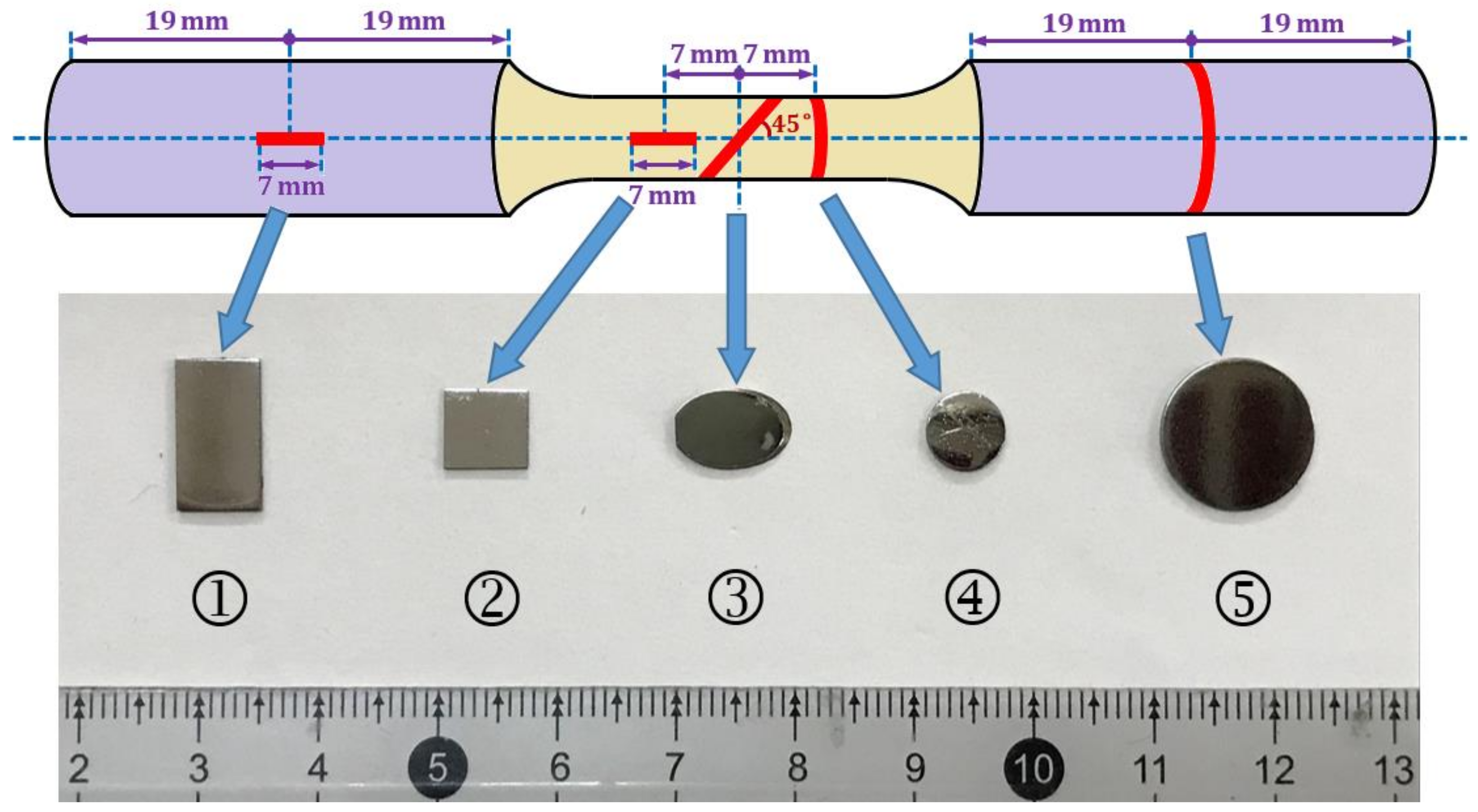
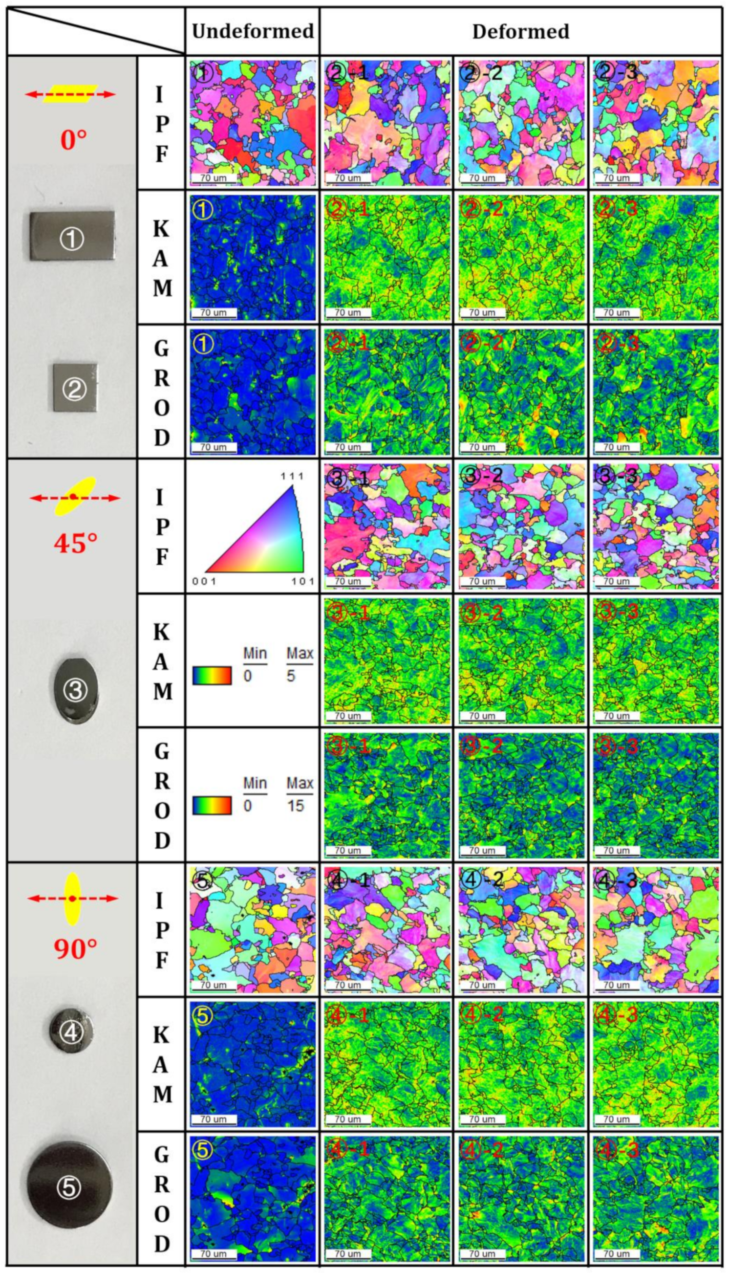
2.2. 2D-EBSD Observations

Two-dimensional electron back-scattered diffraction observations (2D-EBSD) were carried out on five planes ➀–➄ with different angles to loading axis in both clamp sections and gauge section of interrupted Specimen A, whose exact locations are shown in Figure 3. Therein, two planes ➀ and ➄ are located in clamp sections at two ends with angles of 0° and 90° to loading axis, respectively, which are undeformed during the tensile mechanical test. Meanwhile, three other planes ➁, ➂ and ➃ are located in gauge section in the middle with angles of 0°, 45°and 90° to loading axis, respectively, which are uniformly elongated to 12% during the tensile mechanical test. The comparison between ➀ and ➄ is aimed at confirming the isotropic distribution of initial intragranular misorientation before deformation, while the comparison among ➁, ➂ and ➃ is aimed at revealing the isotropic evolution law of intragranular misorientation during deformation.

All the samples for the following 2D-EBSD observations were removed from the interrupted Specimen A by electro discharge cutting method. After the typical grinding procedure, these samples were firstly polished by specified cloth adhered with 3.5, 2.5, 1.5 and 0.5 μm diamond particles for 10–15 min every step and then attached in an aluminum platform and followed by 2–3 h vibratory polishing in Buehler VibroMet 2^® machine (Buehler Group Inc., Lake Bluff, IL, USA) to release the sample surface residual stress. The specified polishing liquid used in Buehler VibroMet 2^® machine contains tiny (~100 nm) SiO₂ particles and acid solution, which can help remove the slight deformation layer in the polished sample surface through coupled mechanical–chemical effects to ensure the Kikuchi patterns quality.

The 2D-EBSD observational region size is set as 200 μm × 200 μm, and the scanning step size is a = 0.8 μm. Then, 2D-EBSD scanning records the orientation information in the observational plane as three Euler angles $\left({\varphi }_1,\varphi ,{\varphi }_2\right)$ point by point through Hough transformation of Kikuchi patterns as shown in Figure 4a,b. The type of field emission scanning electron microscope (SEM) used in this research is TESCAN MIRA 3 LMH^® (TESCAN ORSAY HOLDING a.s., Kohoutovice, Czech Republic). The EBSD camera equipped in SEM platform is Nordly II^® (Oxford Instruments plc., Oxford, UK), and the matched EBSD data collection software is Aztec^® (Oxford Instruments plc., Oxford, UK). All the data were saved in square structure as shown in Figure 4b,c, and then analyzed by OIM Analysis 6.2^® (EDAX Inc., Pleasanton, CA, USA).

For the convenience of calculating misorientation, the Euler angles $\left({\varphi }_1,\varphi ,{\varphi }_2\right)$, which represent three relative rotations between local lattice coordinate ([100], [010], [001]) and global sample coordinate (RD, TD, ND) and are usually converted into the orientation matrix $\mathit{g}$ as shown in Equation (1):

$$\mathit{g}=\left[\begin{array}{ccc}\cos {\varphi }_2& \sin {\varphi }_2& 0\\ -\sin {\varphi }_2& \cos {\varphi }_2& 0\\ 0& 0& 1\end{array}\right]\left[\begin{array}{ccc}1& 0& 0\\ 0& \cos \varphi & \sin \varphi \\ 0& -\sin \varphi & \cos \varphi \end{array}\right]\left[\begin{array}{ccc}\cos {\varphi }_1& \sin {\varphi }_1& 0\\ -\sin {\varphi }_1& \cos {\varphi }_1& 0\\ 0& 0& 1\end{array}\right]$$

(1)

The misorientation $\Delta {\theta }_{\mathrm{A}}^{\mathrm{B}}$ between two different points A and B can then be calculated as shown in Equation (2), where ${\mathit{g}}_{\mathrm{A}}$ and ${\mathit{g}}_{\mathrm{B}}$ represent the orientation matrixes of points A and B, respectively. $S_k{|}_{k=1~24}$ indicate the 24 symmetry operators of BCC lattice, which can be referred to in Refs. [22,48]. The minimum lattice rotation angle of the above 24 equivalent lattice rotation operations converting orientation of point A into orientation of point B is then set as the misorientation $\Delta {\theta }_{\mathrm{A}}^{\mathrm{B}}$ between them.

$$\Delta {\theta }_{\mathrm{A}}^{\mathrm{B}}=\underset{i,j=1~24}{\min }\left[\arccos \left(\frac{\mathrm{trace}\left[\left({\mathit{S}}_i·{\mathit{g}}_{\mathrm{B}}\right)·{\left({\mathit{S}}_j·{\mathit{g}}_{\mathrm{A}}\right)}^{-1}\right]-1}{2}\right)\right]$$

(2)

The parameters for quantifying intragranular misorientation in this research are KAM and GROD. KAM (i, j) is defined as the average misorientation between the kernel point (i, j) and its nearest neighboring points (i−1, j), (i, j−1), (i, j+1), (i+1, j) in the same grain as shown in Figure 4c and Equation (3):

$$KAM\left(i,j\right)\stackrel{\mathrm{def}}{=}\frac{1}{4}\left(\Delta {\theta }_{\left(i,j\right)}^{\left(i-1,j\right)}+\Delta {\theta }_{\left(i,j\right)}^{\left(i,j-1\right)}+\Delta {\theta }_{\left(i,j\right)}^{\left(i,j+1\right)}+\Delta {\theta }_{\left(i,j\right)}^{\left(i+1,j\right)}\right)$$

(3)

where any neighboring points outside the grain boundary will be ignored. Another misorientation parameter GROD (m, n) is defined as the misorientation between the individual point (m, n) and the reference point r in the same grain representing its average orientation, where the detailed calculation method of average orientation can be referred to in Refs. [49,50], as shown in the Figure 4c and Equation (4):

$$GROD\left(m,n\right)\stackrel{\mathrm{def}}{=}\Delta {\theta }_r^{\left(m,n\right)}$$

(4)

After the KAM and GROD values in each EBSD scanning point were calculated, the KAM and GROD distribution maps can be drawn by the software OIM Analysis 6.2^® automatically. Instead of KAM (i, j) and GROD (m, n) sensitive to the local microstructural features, $\overline{KAM}$ and $\overline{GROD}$ averaged over the whole 2D-EBSD observational region (P × Q scanning points) containing multiple grains, as shown in Equation (5), are widely used for measuring the mesoscopic plastic strain in the corresponding 2D-EBSD observational position because they are independent of the local microstructural features.

$$\begin{array}{c}\overline{KAM}\\ \overline{GROD}\end{array}=\frac{1}{P\times Q}{\displaystyle \sum }_{i,m=a}^{P·a}{\displaystyle \sum }_{j,n=a}^{Q·a}\begin{array}{c}KAM\left(i,j\right)\\ GROD\left(m,n\right)\end{array}$$

(5)

3. Experimental Results

The IPF, KAM and GROD maps given by 2D-EBSD observations on different planes with angles of 0°, 45° and 90° to loading axis, respectively, in the gauge section and two clamp sections of interrupted Specimen A are shown in Figure 5. Fe₃C layers distributed in the pearlite phase were not recognized as an independent phase separately by the EBSD data collection software; thus, both ferrite and pearlite phases were identified as the single BCC phase. From the IPF maps, we can see the cross profile of each grain enclosed by grain boundary (GB) on the 2D-EBSD observational plane. Most cross profiles present irregular but equiaxial shapes, and their sizes d range from several to dozens of microns. If the equiaxial grain is regarded as a sphere with diameter of $D_{\mathrm{Grain}}$, the difference among those cross profile sizes d shown in the IPF maps should be attributed to not only the different grain sizes $D_{\mathrm{Grain}}$, but also to the different distances H between 2D-EBSD observational plane and grain center (GC), as shown in both Figure 6 (illustration explaining the geometric relationship between 3D grain size $D_{\mathrm{Grain}}$ and cross profile size d) and Equation (6). On one hand, the larger the grain size $D_{\mathrm{Grain}}$ is, the larger the cross profile size d presents on the 2D-EBSD observational plane when its distance H away from GC is constant. On the other hand, the closer the distance away from GC, the larger the cross profile size d presents on the 2D-EBSD observational plane when the grain size $D_{\mathrm{Grain}}$ is constant.

$$d=\sqrt{D_{\mathrm{Grain}}^2-4H^2}$$

(6)

From the KAM and GROD maps, we can see that intragranular misorientation levels are relatively low in two underformed clamp sections but high in deformed gauge section. The intragranular misorientation values averaged over the whole 2D-EBSD observational region containing multiple grains are drawn in Figure 7. The subscript “0” stands for average $\overline{KAM}$ and $\overline{GROD}$ values measured from undeformed clamp sections, different from those from deformed gauge section. For two undeformed clamp sections, the average $\overline{KAM}$ and $\overline{GROD}$ values measured on 2D-EBSD observational planes with angles of 0° and 90° to loading axis, respectively, are almost the same. This reveals the isotropic distribution law of initial intragranular misorientation. For the deformed gauge section, the average $\overline{KAM}$ and $\overline{GROD}$ values repeatedly measured on 2D-EBSD observational planes with angles of 0°, 45° and 90° to loading axis are also almost the same. This reveals the isotropic evolution law of intragranular misorientation during the tensile deformation. In previous works, the linear evolution law of intragranular misorientation during the tensile deformation has been widely confirmed by Refs. [4,5,6,7,8], which laid the foundation for indicating the mesoscopic plastic strain by average $\overline{KAM}$ and $\overline{GROD}$ values. Furthermore, the isotropic evolution law of intragranular misorientation confirmed by this research ensures that average $\overline{KAM}$ and $\overline{GROD}$ values are independent of the 2D-EBSD observational planes selection. This is quite an important property because $\overline{KAM}$ and $\overline{GROD}$ can only serve as objective plasticity indicators if their values are determined by mesoscopic plastic strain while not affected by observational plane selection.

4. Theoretical Discussions

The isotropic linear evolution law of intragranular misorientation (quantified by $\overline{KAM}$ and $\overline{GROD}$) in deformed polycrystalline metals with uniform equiaxial grains has been confirmed by this research as well as by other studies [4,5,6,7,8] as an important experimental phenomenon. To explain the linear evolution law of intragranular misorientation reported by other studies [4,5,6,7,8], our previous work [45] has established a preliminary theoretical model based on several fundamental assumptions in the 2D case. However, this 2D polycrystalline plasticity model has not yet been generalized to the 3D case and thus cannot explain the isotropic evolution law of intragranular misorientation observed in our experimental results here. To address the above issue, a modified 3D polycrystalline plasticity model explaining isotropic linear evolution law of intragranular misorientation was then developed.

4.1. Fundamental Assumptions

To establish the 3D polycrystalline plasticity model for explaining isotropic linear evolution of intragranular misorientation, six fundamental assumptions listed below should be made in advance to simplify the mathematical derivation process of $\overline{KAM}$ and $\overline{GROD}$ evolution law, as shown in Figure 8.

(1)

The intragranular plastic distortion ${\mathit{\beta }}^{\mathrm{p}}$ follows the crystal plasticity theory. No more than five independent slip factors (${\overrightarrow{\mathit{s}}}^1$, ${\overrightarrow{\mathit{n}}}^1$)~(${\overrightarrow{\mathit{s}}}^5$, ${\overrightarrow{\mathit{n}}}^5$) are activated to undertake the intragranular plastic distortion, which are selected from those potential slip factors of specific lattice at a given temperature with the highest five resolved shear stresses ${\tau }^1$~${\tau }^5$ under the mesoscopic stress $\overline{\mathit{\sigma }}$ applied in RVE. The plastic strain is small enough to ensure that the additive decomposition is applicable to the distortion tensor ${\mathit{\beta }}^{\mathrm{p}}$ and the activated slip factors (${\overrightarrow{\mathit{s}}}^{\alpha }$, ${\overrightarrow{\mathit{n}}}^{\alpha }$) can be regarded as approximately fixed during the deformation.

(2)

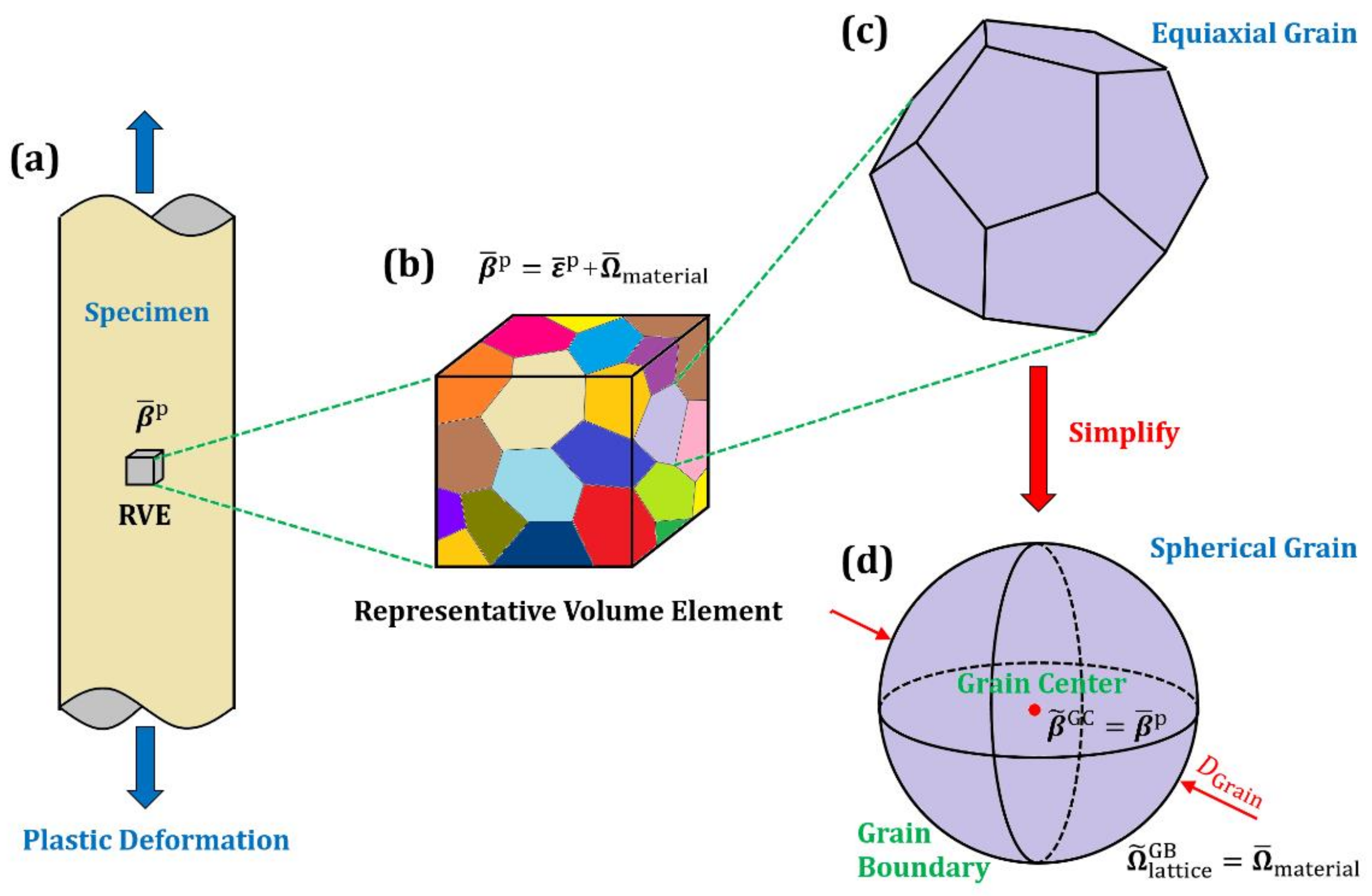
The RVE containing multiple grains can be regarded as homogeneous and isotropic, while its mesoscopic plastic strain ${\overline{\mathit{\epsilon }}}^{\mathrm{p}}$ and mesoscopic stress $\overline{\mathit{\sigma }}$ follow the classical J₂ finite strain plasticity theory: ${\overline{\mathit{\epsilon }}}^{\mathrm{p}}$∥$\overline{\mathit{\sigma }}\prime$, which requires that three principal directions of deviatoric stress tensor $\overline{\mathit{\sigma }}\prime$ and the ratio among three principal stresses of stress tensor $\overline{\mathit{\sigma }}$ are fixed during the whole deformation history.

(3)

The residual material distortion ${\tilde{\mathit{\beta }}}^{\mathrm{GC}}$ at the GC made up of microscopic plastic distortion ${\mathit{\beta }}^{\mathrm{p}}\left(0\right)$ and residual lattice rotation ${\tilde{\Omega }}_{\mathrm{lattice}}\left(0\right)$ is equal to the mesoscopic plastic distortion ${\overline{\mathit{\beta }}}^{\mathrm{p}}$ of RVE, which is the same as that in Taylor’s polycrystalline model.

(4)

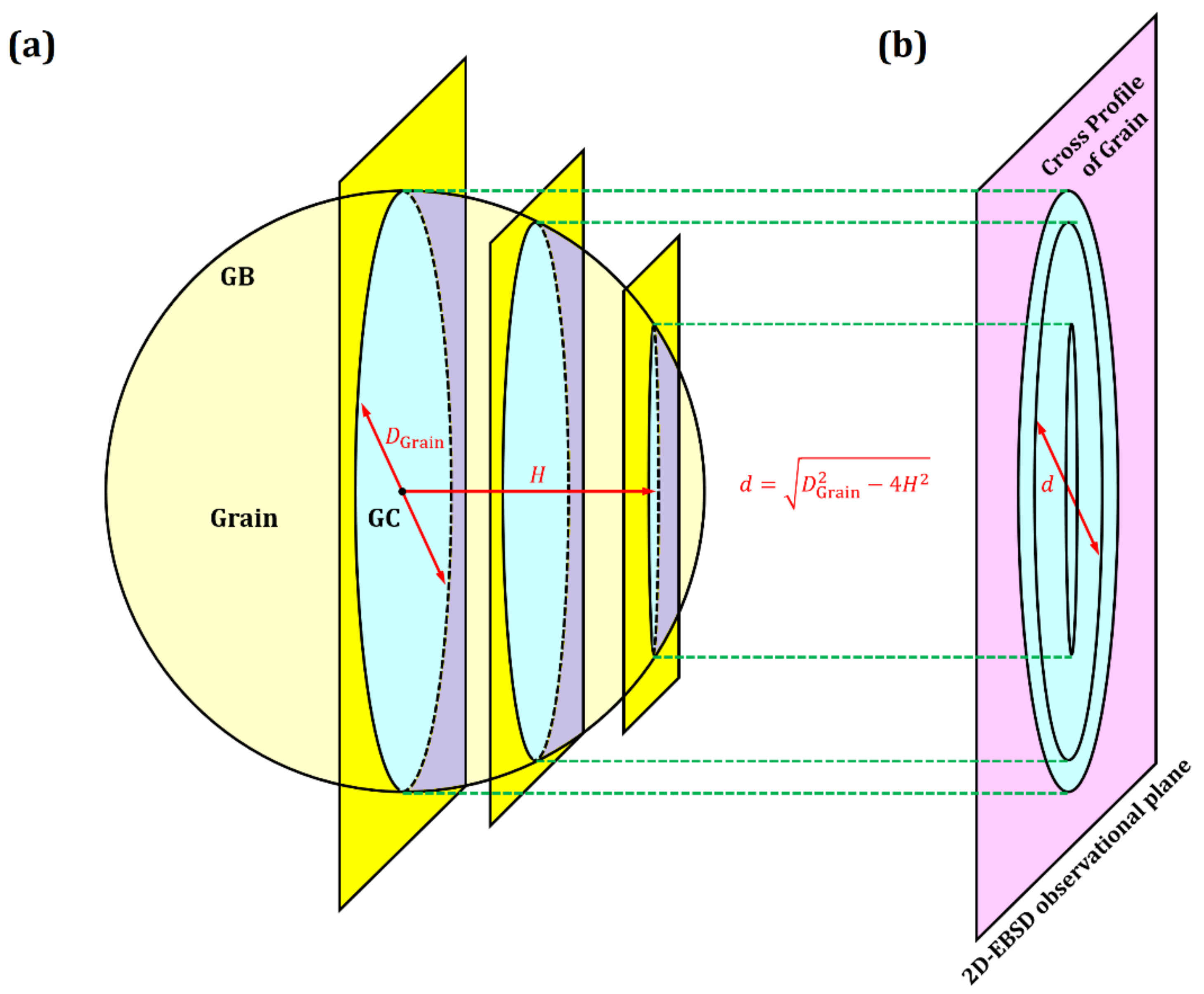
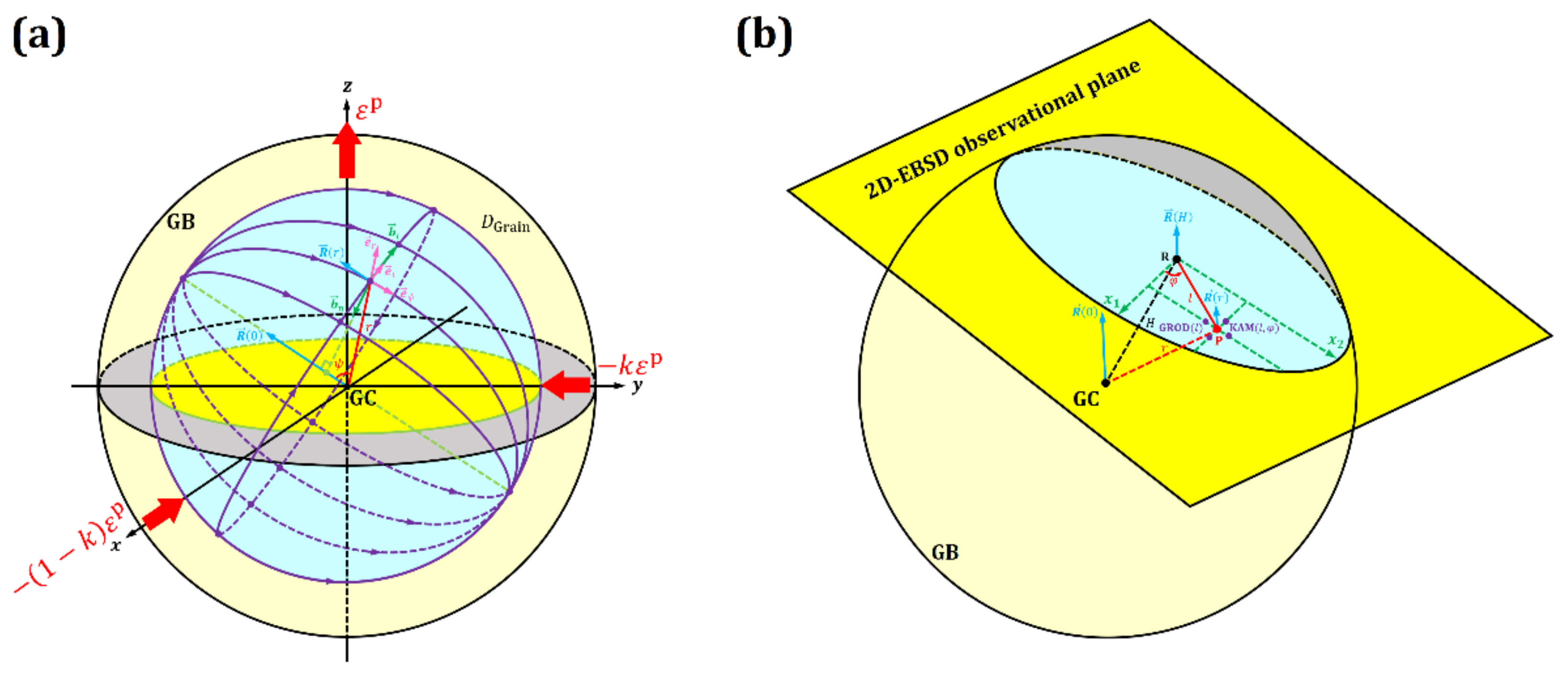
Each equaxial grain can be simplified as a sphere with the same diameter of $D_{\mathrm{Grain}}$, while the distance between its GC and the 2D-EBSD observational plane is H. For each spherical grain cut by the 2D-EBSD observational plane, the ratio $2H/D_{\mathrm{Grain}}$ is a random variable ranging from 0 to 1.

(5)

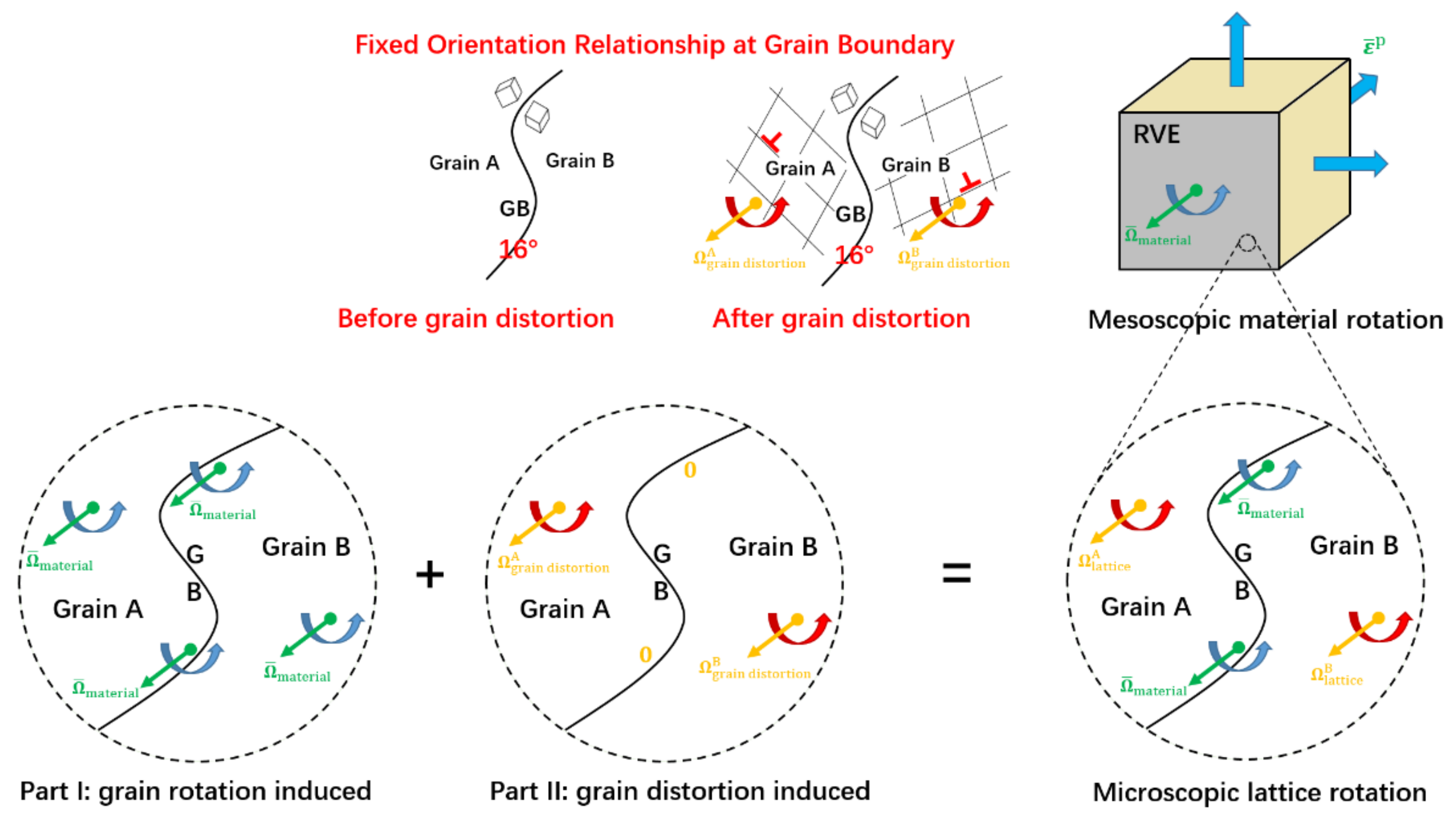
The residual lattice rotation ${\tilde{\Omega }}_{\mathrm{lattice}}^{\mathrm{GB}}$ near the GB is close to the mesoscopic material rotation ${\overline{\Omega }}_{\mathrm{material}}$ of RVE due to the restraint from the fixed orientation relationship between the two sides of GB, as explained by Figure 9. The lattice rotation inside each grain is induced by two parts: one is induced by the overall grain rotation synchronized with the mesoscopic material rotation, and another is induced by the grain distortion accompanied with dislocations slip. Therein, the lattice rotation induced by the grain distortion must be zero near the GB; otherwise, the fixed orientation relationship between the two sides of GB will be broken (e.g., the GB misorientation angle will be changed). Taking this into account, the residual lattice rotation at the GB should be the same as the mesoscopic material rotation, since the other part must be equal to zero. A deeper physical reason is that the interior dislocations cannot be absorbed or released by those GBs at the room temperature.

(6)

The intragranular residual lattice rotation ${\tilde{\Omega }}_{\mathrm{lattice}}$ decreases from GC to GB along the grain radius r linearly and isotropically in spherical grains:${\tilde{\Omega }}_{\mathrm{lattice}}={\tilde{\Omega }}_{\mathrm{lattice}}\left(r\right)$ and ${\partial }^2{\tilde{\Omega }}_{\mathrm{lattice}}/\partial r^2=\mathbf{0}$.

Figure 9. The explanation for the fixed orientation relationship between two sides of GB.

Figure 9. The explanation for the fixed orientation relationship between two sides of GB.

4.2. Establishment of 3D Polycrystalline Plasticity Model

The intragranular residual material distortion $\tilde{\mathit{\beta }}$ after unloading is made up of two parts: the intragranular plastic distortion ${\mathit{\beta }}^{\mathrm{p}}$ and the intragranular residual lattice rotation ${\tilde{\Omega }}_{\mathrm{lattice}}$. Further, the intragranular plastic distortion ${\mathit{\beta }}^{\mathrm{p}}$ is undertaken by the crystallographic slip ${\gamma }_m$ in no more than five independent slip factors (${\overrightarrow{\mathit{s}}}^m$, ${\overrightarrow{\mathit{n}}}^m$) according to Assumption (1), where the unit vector ${\overrightarrow{\mathit{s}}}^m$ represents slip direction, the unit vector ${\overrightarrow{\mathit{n}}}^m$ represents normal direction of slip plane, and m = 1–5, as shown in Equation (7). In this equation, eight quantities ${\gamma }_1$~${\gamma }_5$ and ${\theta }_1$~${\theta }_3$ are unknown, while eight independent sub-equations are given. Therefore, a unique solution can be determined only if the five activated slip factors (${\overrightarrow{\mathit{s}}}^1$, ${\overrightarrow{\mathit{n}}}^1$)~(${\overrightarrow{\mathit{s}}}^5$, ${\overrightarrow{\mathit{n}}}^5$) and the intragranular residual material distortion $\tilde{\mathit{\beta }}$ are known in advance.

$$\stackrel{\tilde{\mathit{\beta }}}{\overbrace{\left[\begin{array}{ccc}-{\epsilon }_1^{\mathrm{p}}& {\gamma }_3^{\mathrm{p}}+{\omega }_3& {\gamma }_2^{\mathrm{p}}-{\omega }_2\\ {\gamma }_3^{\mathrm{p}}-{\omega }_3& -{\epsilon }_2^{\mathrm{p}}& {\gamma }_1^{\mathrm{p}}+{\omega }_1\\ {\gamma }_2^{\mathrm{p}}+{\omega }_2& {\gamma }_1^{\mathrm{p}}-{\omega }_1& {\epsilon }_1^{\mathrm{p}}+{\epsilon }_2^{\mathrm{p}}\end{array}\right]}}=\stackrel{{\mathit{\beta }}^{\mathrm{p}}}{\overbrace{\left({\gamma }_1{\overrightarrow{\mathit{s}}}^1{\overrightarrow{\mathit{n}}}^1+{\gamma }_2{\overrightarrow{\mathit{s}}}^2{\overrightarrow{\mathit{n}}}^2+{\gamma }_3{\overrightarrow{\mathit{s}}}^3{\overrightarrow{\mathit{n}}}^3+{\gamma }_4{\overrightarrow{\mathit{s}}}^4{\overrightarrow{\mathit{n}}}^4+{\gamma }_5{\overrightarrow{\mathit{s}}}^5{\overrightarrow{\mathit{n}}}^5\right)}}+\stackrel{{\tilde{\Omega }}_{\mathrm{lattice}}}{\overbrace{\left[\begin{array}{ccc}0& {\theta }_3& -{\theta }_2\\ -{\theta }_3& 0& {\theta }_1\\ {\theta }_2& -{\theta }_1& 0\end{array}\right]}}$$

(7)

A coordinate system should be established in advance to help describe the evolution of various intragranular physical fields during the grain distortion, and the origin of the coordinate system is naturally located at the GC of each grain. To simplify the expression of mesoscopic plastic distortion ${\overline{\mathit{\beta }}}^{\mathrm{p}}$ of RVE, three axes x, y and z of the coordinate system are parallel to three principal directions of mesoscopic plastic strain ${\overline{\mathit{\epsilon }}}^{\mathrm{p}}$, where the shear plastic strain components ${\gamma }_1^{\mathrm{p}}$~${\gamma }_3^{\mathrm{p}}$ will be equal to zero in that case. At the same time, the mesoscopic stress $\overline{\mathit{\sigma }}$ applied in RVE is made up of the deviatoric part $\overline{\mathit{\sigma }}\prime$ and the hydrostatic part, while the deviatoric part $\overline{\mathit{\sigma }}\prime$ should meet the requirement of ${\overline{\mathit{\epsilon }}}^{\mathrm{p}}$∥$\overline{\mathit{\sigma }}\prime$ according to J₂ finite strain plasticity theory in Assumption (2). The detailed components of ${\overline{\mathit{\beta }}}^{\mathrm{p}}$ and $\overline{\mathit{\sigma }}$ are shown in Equation (8), where ${\epsilon }^{\mathrm{p}}$ is the maximum principal plastic strain along z axis and 0 ≤ k ≤ 1 is the variable controlling the ratio between another two principal plastic strains along the x and y axes. In particular, k is equal to 1/2 in the uniaxial tension case.

$${\overline{\mathit{\beta }}}^{\mathrm{p}}=\stackrel{{\overline{\mathit{\epsilon }}}^{\mathrm{p}}}{\overbrace{\left[\begin{array}{ccc}-\left(1-k\right){\epsilon }^p& 0& 0\\ 0& -k{\epsilon }^p& 0\\ 0& 0& {\epsilon }^p\end{array}\right]}}+\stackrel{{\overline{\Omega }}_{\mathrm{material}}}{\overbrace{\left[\begin{array}{ccc}0& {\omega }_3& -{\omega }_2\\ -{\omega }_3& 0& {\omega }_1\\ {\omega }_2& -{\omega }_1& 0\end{array}\right]}}, \overline{\mathit{\sigma }}=\stackrel{\overline{\mathit{\sigma }}\prime }{\overbrace{\left[\begin{array}{ccc}-\left(1-k\right)\sigma & 0& 0\\ 0& -k\sigma & 0\\ 0& 0& \sigma \end{array}\right]}}+\left[\begin{array}{ccc}\eta & 0& 0\\ 0& \eta & 0\\ 0& 0& \eta \end{array}\right]$$

(8)

According to Assumption (3), the residual material distortion ${\tilde{\mathit{\beta }}}^{\mathrm{GC}}$ at the GC made up of microscopic plastic distortion ${\mathit{\beta }}^{\mathrm{p}}\left(0\right)$ and residual lattice rotation ${\tilde{\Omega }}_{\mathrm{lattice}}\left(0\right)$ is equal to the mesoscopic plastic distortion ${\overline{\mathit{\beta }}}^{\mathrm{p}}$ of RVE. Then, Equation (7) can be applied to the GC and generates to Equation (9).

$${\overline{\mathit{\beta }}}^{\mathrm{p}}={\overline{\mathit{\epsilon }}}^{\mathrm{p}}+{\overline{\Omega }}_{\mathrm{material}}={\tilde{\mathit{\beta }}}^{\mathrm{GC}}=\stackrel{{\mathit{\beta }}^{\mathrm{p}}\left(0\right)}{\overbrace{\left({\gamma }_1{\overrightarrow{\mathit{s}}}^1{\overrightarrow{\mathit{n}}}^1+{\gamma }_2{\overrightarrow{\mathit{s}}}^2{\overrightarrow{\mathit{n}}}^2+{\gamma }_3{\overrightarrow{\mathit{s}}}^3{\overrightarrow{\mathit{n}}}^3+{\gamma }_4{\overrightarrow{\mathit{s}}}^4{\overrightarrow{\mathit{n}}}^4+{\gamma }_5{\overrightarrow{\mathit{s}}}^5{\overrightarrow{\mathit{n}}}^5\right)}}+\stackrel{{\tilde{\Omega }}_{\mathrm{lattice}}\left(0\right)}{\overbrace{\left[\begin{array}{ccc}0& {\theta }_3\left(0\right)& -{\theta }_2\left(0\right)\\ -{\theta }_3\left(0\right)& 0& {\theta }_1\left(0\right)\\ {\theta }_2\left(0\right)& -{\theta }_1\left(0\right)& 0\end{array}\right]}}$$

(9)

According to Assumptions (4) and (5), the residual lattice rotation ${\tilde{\Omega }}_{\mathrm{lattice}}^{\mathrm{GB}}={\tilde{\Omega }}_{\mathrm{lattice}}\left(D_{\mathrm{Grain}}/2\right)$ near the GB of each spherical grain is close to the mesoscopic material rotation ${\overline{\Omega }}_{\mathrm{material}}$ of RVE. Then, Equation (10) connecting the mesoscopic plastic strain ${\overline{\mathit{\epsilon }}}^{\mathrm{p}}$ of RVE to the intragranular misorientation ${\tilde{\Omega }}_{\mathrm{lattice}}\left(0\right)-{\tilde{\Omega }}_{\mathrm{lattice}}\left(D_{\mathrm{Grain}}/2\right)$ between GC and GB of each grain can be established based on Equation (9). From this equation, we can see that the intragranular misorientation will be mainly determined by mesoscopic plastic strain ${\overline{\mathit{\epsilon }}}^{\mathrm{p}}$ rather than ${\overline{\Omega }}_{\mathrm{material}}$ of RVE if Assumption (5) is correct.

$$\stackrel{{\overline{\mathit{\epsilon }}}^{\mathrm{p}}}{\overbrace{\left[\begin{array}{ccc}-\left(1-k\right){\epsilon }^{\mathrm{p}}& 0& 0\\ 0& -k{\epsilon }^{\mathrm{p}}& 0\\ 0& 0& {\epsilon }^{\mathrm{p}}\end{array}\right]}}=\stackrel{{\mathit{\beta }}^{\mathrm{p}}\left(0\right)}{\overbrace{\left({\gamma }_1{\overrightarrow{\mathit{s}}}^1{\overrightarrow{\mathit{n}}}^1+{\gamma }_2{\overrightarrow{\mathit{s}}}^2{\overrightarrow{\mathit{n}}}^2+{\gamma }_3{\overrightarrow{\mathit{s}}}^3{\overrightarrow{\mathit{n}}}^3+{\gamma }_4{\overrightarrow{\mathit{s}}}^4{\overrightarrow{\mathit{n}}}^4+{\gamma }_5{\overrightarrow{\mathit{s}}}^5{\overrightarrow{\mathit{n}}}^5\right)}}+\left[{\tilde{\Omega }}_{\mathrm{lattice}}\left(0\right)-{\tilde{\Omega }}_{\mathrm{lattice}}\left(D_{\mathrm{Grain}}/2\right)\right]$$

(10)

To calculate the intragranular misorientation ${\tilde{\Omega }}_{\mathrm{lattice}}\left(0\right)-{\tilde{\Omega }}_{\mathrm{lattice}}\left(D_{\mathrm{Grain}}/2\right)$ between GC and GB determined by the mesoscopic plastic strain ${\overline{\mathit{\epsilon }}}^{\mathrm{p}}$, the five activated slip factors (${\overrightarrow{\mathit{s}}}^1$, ${\overrightarrow{\mathit{n}}}^1$)~(${\overrightarrow{\mathit{s}}}^5$, ${\overrightarrow{\mathit{n}}}^5$) should be determined first. For the type 40Cr low alloy steel made up of ferrite and pearlite phases used in this research, the potential slip system of BCC lattice at room temperature is mainly the {110}<111> including twelve equivalent slip factors $\left(h^{\alpha } k^{\alpha } l^{\alpha }\right)\left[u^{\alpha } v^{\alpha } w^{\alpha }\right]$ as shown in

Table 2. Twelve equivalent slip factors of BCC lattice at room temperature.

α	1	2	3	4	5	6	7	8	9	10	11	12
(hα kα lα)	(110)	(110)	$(1\stackrel{-}{1}0)$	$(1\stackrel{-}{1}0)$	(101)	(101)	$(10\stackrel{-}{1})$	$(10\stackrel{-}{1})$	(011)	(011)	$(01\stackrel{-}{1})$	$(01\stackrel{-}{1})$
[uα vα wα]	$[1\stackrel{-}{1}1]$	$[\stackrel{-}{1}11]$	[111]	$[11\stackrel{-}{1}]$	$[11\stackrel{-}{1}]$	$[\stackrel{-}{1}11]$	$[1\stackrel{-}{1}1]$	[111]	$[1\stackrel{-}{1}1]$	$[11\stackrel{-}{1}]$	$[\stackrel{-}{1}11]$	[111]

.

The resolved shear stresses ${\tau }^{\alpha }$ of twelve potential equivalent slip factors $\left(h^{\alpha } k^{\alpha } l^{\alpha }\right)\left[u^{\alpha } v^{\alpha } w^{\alpha }\right]$ in one grain with the orientation of $\mathit{g}\left({\varphi }_1,\varphi ,{\varphi }_2\right)$ under mesoscopic stress $\overline{\mathit{\sigma }}$ applied in RVE can be calculated as shown in Equation (11). The five activated slip factors $\left({\overrightarrow{\mathit{s}}}^m,{\overrightarrow{\mathit{n}}}^m\right){|}_{m=1~5}$ for undertaking the intragranular plastic distortion ${\mathit{\beta }}^{\mathrm{p}}$ are selected from the twelve potential slip factors $\left({\overrightarrow{\mathit{s}}}^{\alpha },{\overrightarrow{\mathit{n}}}^{\alpha }\right){|}_{\alpha =1~12}$ with the highest five resolved shear stresses among ${\tau }^1$~${\tau }^{12}$ according to Assumption (1).

$${\overrightarrow{\mathit{s}}}^{\alpha }={\mathit{g}}^T·\left[\begin{array}{c}{u}^{\alpha }\\ v^{\alpha }\\ w^{\alpha }\end{array}\right],\hspace{1em}{\overrightarrow{\mathit{n}}}^{\alpha }={\mathit{g}}^T·\left[\begin{array}{c}{h}^{\alpha }\\ k^{\alpha }\\ l^{\alpha }\end{array}\right],\hspace{1em}{\tau }^{\alpha }=\overline{\mathit{\sigma }}\prime :\left({\overrightarrow{\mathit{s}}}^{\alpha }{\overrightarrow{\mathit{n}}}^{\alpha }\right),\hspace{1em}\left({\overrightarrow{\mathit{s}}}^m, {\overrightarrow{\mathit{n}}}^m\right){|}_{m=1~5}=\left({\overrightarrow{\mathit{s}}}^{\alpha }, {\overrightarrow{\mathit{n}}}^{\alpha }\right){|}_{{\tau }^{\alpha } \in \mathrm{highest}\mathrm{five} \left\{{\tau }^1~{\tau }^{12}\right\}}$$

(11)

Once the intragranular misorientation ${\tilde{\Omega }}_{\mathrm{lattice}}\left(0\right)-{\tilde{\Omega }}_{\mathrm{lattice}}\left(D_{\mathrm{Grain}}/2\right)$ between GC and GB of each grain under the mesoscopic plastic strain ${\overline{\mathit{\epsilon }}}^{\mathrm{p}}$ is determined, the relative lattice rotation vector $\overrightarrow{\mathit{R}}\left(r\right)$ can be then introduced to describe the distribution of intragranular misorientation ${\tilde{\Omega }}_{\mathrm{lattice}}\left(r\right)-{\tilde{\Omega }}_{\mathrm{lattice}}\left(D_{\mathrm{Grain}}/2\right)$ along the grain radius r according to Assumption (6), as shown in Equation (12)

$$\overrightarrow{\mathit{R}}\left(r\right)=\stackrel{R_1\left(r\right)}{\overbrace{\left[{\theta }_1\left(r\right)-{\theta }_1\left(D_{\mathrm{Grain}}/2\right)\right]}}{\overrightarrow{\mathit{e}}}_1+\stackrel{R_2\left(r\right)}{\overbrace{\left[{\theta }_2\left(r\right)-{\theta }_2\left(D_{\mathrm{Grain}}/2\right)\right]}}{\overrightarrow{\mathit{e}}}_2+\stackrel{R_3\left(r\right)}{\overbrace{\left[{\theta }_3\left(r\right)-{\theta }_3\left(D_{\mathrm{Grain}}/2\right)\right]}}{\overrightarrow{\mathit{e}}}_3=\left(1-\frac{2r}{D_{\mathrm{Grain}}}\right)\overrightarrow{\mathit{R}}\left(0\right)$$

(12)

4.3. Linear Evolution Law of Intragranular Misorientation

After establishing the 3D polycrystalline plasticity model, the next issue is to clarify the linear evolution law of intragranular misorientation with the mesoscopic plastic strain ${\overline{\mathit{\epsilon }}}^{\mathrm{p}}$ of RVE based on Equations (10) and (11), while the intragranular misorientation distribution $\overrightarrow{\mathit{R}}\left(r\right)$ is controlled by $\overrightarrow{\mathit{R}}\left(0\right)$ at the GC completely according to Equation (12). Therein, Equation (10) is a system of linear equations; thus, both the crystallographic slip amounts ${\gamma }_1$~${\gamma }_5$ and relative lattice rotation components $R_1\left(0\right)$~$R_3\left(0\right)$ at the GC will be proportional to the maximum principal plastic strain ${\epsilon }^{\mathrm{p}}$ of RVE. However, the change rates of lattice rotation components with the maximum principal plastic strain $C_{1~3}=\mathrm{d}{R}_{1~3}\left(0\right) /\mathrm{d}{\epsilon }^{\mathrm{p}}$ will be influenced by the variable k controlling the ratio between another two principal plastic strains, as well as the lattice orientation ${\varphi }_1,\varphi ,{\varphi }_2$ controlling the grain activated slip factors $\left({\overrightarrow{\mathit{s}}}^m,{\overrightarrow{\mathit{n}}}^m\right){|}_{m=1~5}$.

The analytical expression of $R_{1~3}\left(0\right)=C_{1~3}·{\epsilon }^{\mathrm{p}}$ is too complex to be derived from Equation (10) directly. Therefore, the numerical solutions to Equation (10) were achieved by MATLAB, instead of analytical approach. Figure 10 displayed the numerical solutions to Equation (10) under four special cases: (a) ${\varphi }_1=\varphi ={\varphi }_2=\pi /4$; (b) ${\varphi }_1=\varphi =\pi /4, {\varphi }_2=\pi /5$; (c) ${\varphi }_1=\pi /5, \varphi ={\varphi }_2=\pi /4$; (d)$\varphi =\pi /5,{\varphi }_1={\varphi }_2=\pi /4$. For each case, k value was set as 0.0, 0.5 and 1.0, respectively. The calculation results shown in Figure 10 help us confirm that the lattice rotation components $R_{1~3}\left(0\right)$ at the GC are proportional to the maximum principal plastic strain ${\epsilon }^{\mathrm{p}}$ of RVE, while the lattice rotation change rates $\mathrm{d}{R}_{1~3}\left(0\right)/\mathrm{d}{\epsilon }^{\mathrm{p}}$ are functions of both variable k and Euler angles: $C_{1~3}=C_{1~3}\left(k, {\varphi }_1,\varphi ,{\varphi }_2\right)$.

After confirming the linear relationship between relative lattice rotation components $R_{1~3}\left(0\right)$ at the GC and the maximum principal plastic strain ${\epsilon }^{\mathrm{p}}$ of RVE, the linear evolution law of relative lattice rotation vector $\overrightarrow{\mathit{R}}\left(0\right)$ at the GC can be then determined as shown in Equation (13). The ratio among $C_1$, $C_2$ and $C_3$ is fixed once the variable k and Euler angles ${\varphi }_1,\varphi ,{\varphi }_2$ are fixed (the fixed k corresponds to the proportional loading case of RVE), which means that the direction of relative lattice rotation vector $\overrightarrow{\mathit{R}}\left(0\right)$ at the GC is fixed in the proportional loading case of RVE. At the same time, the relative lattice rotation angle $\left|\overrightarrow{\mathit{R}}\left(0\right)\right|$ is proportional to the maximum principal plastic strain ${\epsilon }^{\mathrm{p}}$ of RVE: $\left|\overrightarrow{\mathit{R}}\left(0\right)\right|=C·{\epsilon }^{\mathrm{p}}$, and the resultant lattice rotation change rate C is the square root of the quadratic sum of three component lattice rotation change rates $C_1$, $C_2$ and $C_3$: $C=\sqrt{C_1^2+C_2^2+C_3^2}$. As a natural result, the resultant C also depends on the variable k and Euler angles ${\varphi }_1,\varphi ,{\varphi }_2$: $C=C\left(k, {\varphi }_1,\varphi ,{\varphi }_2\right)$.

$$\overrightarrow{\mathit{R}}\left(0\right)=\stackrel{R_1\left(0\right)}{\overbrace{C_1\left(k, {\varphi }_1,\varphi ,{\varphi }_2\right){\epsilon }^{\mathrm{p}}}}{\overrightarrow{\mathit{e}}}_1+\stackrel{R_2\left(0\right)}{\overbrace{C_2\left(k, {\varphi }_1,\varphi ,{\varphi }_2\right){\epsilon }^{\mathrm{p}}}}{\overrightarrow{\mathit{e}}}_2+\stackrel{R_3\left(0\right)}{\overbrace{C_3\left(k, {\varphi }_1,\varphi ,{\varphi }_2\right){\epsilon }^{\mathrm{p}}}}{\overrightarrow{\mathit{e}}}_3, \left|\overrightarrow{\mathit{R}}\left(0\right)\right|=\stackrel{=\sqrt{C_1^2+C_2^2+C_3^2}}{\overbrace{C\left(k, {\varphi }_1,\varphi ,{\varphi }_2\right)}}{\epsilon }^{\mathrm{p}}$$

(13)

Furthermore, the influence of variable k and Euler angles ${\varphi }_1,\varphi ,{\varphi }_2$ on lattice rotation change rates $C_{1~3}\left(k, {\varphi }_1,\varphi ,{\varphi }_2\right)$ was investigated through numerical calculation of another five special cases. For each case, variable k and two of the Euler angles $\varphi ,{\varphi }_2$ are fixed: (a) $k=0.25, \varphi ={\varphi }_2=\pi /4$; (b) $k=0.75, \varphi ={\varphi }_2=\pi /4$; (c) $k=0.50, \varphi ={\varphi }_2=\pi /4$; (d)$k=0.50, \varphi =\pi /5, {\varphi }_2=\pi /4$; (e) $k=0.50, \varphi =\pi /4, {\varphi }_2=\pi /5$, and another Euler angle ${\varphi }_1$ ranges from 0° to 360°, which describes the spatial rotation of crystallographic lattice and potential slip factors $\left({\overrightarrow{\mathit{s}}}^{\alpha },{\overrightarrow{\mathit{n}}}^{\alpha }\right){|}_{\alpha =1~12}$ along the z axis (the direction of maximum principal plastic strain ${\epsilon }^{\mathrm{p}}$). The calculation results are shown in Figure 11, from which we can see not only the dependence of $C_{1~3}$ on both variable k and Euler angles ${\varphi }_1,\varphi ,{\varphi }_2$, but also an interesting phenomenon in $C_{1~3}$ evolution with the change of Euler angle ${\varphi }_1$.

The interesting phenomenon mentioned above is as follows. The $C_{1~3}$ values will suddenly “jump” with the change of Euler angle ${\varphi }_1$ if the variable k ≠ 0.5 as shown in Figure 11a,b, while the $C_{1~2}$ values will smoothly change in a sinusoidal way and the $C_3$ value will keep constant with the change of Euler angle ${\varphi }_1$ if the variable k = 0.5 as shown in Figure 11c–e. This is because the two principal deviatoric stresses $-\left(1-k\right)\sigma$ along the x axis and $-k\sigma$ along the y axis of mesoscopic stress $\overline{\mathit{\sigma }}$ are unequal if k ≠ 0.5, in which case the activated slip factors will naturally vary with the spatial rotation of crystallographic lattice along the z axis. On the contrary, if the mesoscopic stress $\overline{\mathit{\sigma }}$ is transversely isotropic in the x-O-y plane when k = 0.5, then the activated slip factors will be fixed during the spatial rotation of crystallographic lattice along the z axis, and the corresponding $\overrightarrow{\mathit{R}}\left(0\right)$ obtained from Equations (10) and (11) under the same mesoscopic plastic strain ${\overline{\mathit{\epsilon }}}^{\mathrm{p}}$ will rotate along the z axis synchronously with the change of Euler angle ${\varphi }_1$. Therefore, the $C_{1~2}$ values smoothly change in a sinusoidal way and the $C_3$ value keeps constant according to their roles in $\overrightarrow{\mathit{R}}\left(0\right)$ as shown in Equation (13).

4.4. Isotropic Evolution Law of Average $\overline{KAM}$ and $\overline{GROD}$

After clarifying the linear evolution law of intragranular misorientation $\overrightarrow{\mathit{R}}\left(0\right)$ at the GC as well as its distribution $\overrightarrow{\mathit{R}}\left(r\right)$ associated with the mesoscopic plastic strain ${\overline{\mathit{\epsilon }}}^{\mathrm{p}}$ of RVE, the intragranular geometrically necessary dislocation ${\mathit{\rho }}_{\mathrm{GND}}\left(\psi \right)$ and its evolution with maximum principal plastic strain ${\epsilon }^{\mathrm{p}}$ can then be determined by the continuum dislocation theory [41,42,43] as shown in Equation (14) and Figure 12a. The detailed derivation of Equation (14) can be referred to in Appendix A.

$${\mathit{\rho }}_{\mathrm{GND}}\left(\psi \right)={\tilde{\Omega }}_{\mathrm{lattice}}\left(r\right)\times \nabla =\frac{2\left|\overrightarrow{\mathit{R}}\left(0\right)\right|}{b{D}_{\mathrm{Grain}}}\left({\overrightarrow{\mathit{b}}}_{\mathrm{n}}{\overrightarrow{\mathit{e}}}_{\psi }-\cos \psi {\overrightarrow{\mathit{b}}}_{\mathrm{t}}{\overrightarrow{\mathit{e}}}_{\mathrm{t}}\right)=\stackrel{{\rho }_{\mathrm{GND}}}{\overbrace{\frac{2C\left(k, {\varphi }_1,\varphi ,{\varphi }_2\right)·{\epsilon }^p}{b{D}_{\mathrm{Grain}}}}}\left(\stackrel{\mathrm{longitude}}{\overbrace{{\overrightarrow{\mathit{b}}}_{\mathrm{n}}{\overrightarrow{\mathit{e}}}_{\psi }}}-\stackrel{\mathrm{latitude}}{\overbrace{\cos \psi {\overrightarrow{\mathit{b}}}_{\mathrm{t}}{\overrightarrow{\mathit{e}}}_{\mathrm{t}}}}\right)$$

(14)

In the above expression, ${\mathit{\rho }}_{\mathrm{GND}}$ reflects the intragranular geometrically necessary dislocation density proportional to the maximum principal plastic strain ${\epsilon }^{\mathrm{p}}$ but is inversely proportional to the grain diameter $D_{\mathrm{Grain}}$ [51], where the dependence of its change rate $C\left(k, {\varphi }_1,\varphi ,{\varphi }_2\right)$ on the grain orientation has been confirmed by Ref. [52]. $\psi$ is the angle between the radius vector $\overrightarrow{\mathit{r}}$ and the relative lattice rotation vector $\overrightarrow{\mathit{R}}\left(0\right)$ at the GC. At the same time, ${\overrightarrow{\mathit{b}}}_{\mathrm{t}}$ is the Burgers vector perpendicular to both $\overrightarrow{\mathit{R}}\left(0\right)$ and $\overrightarrow{\mathit{r}}$, and ${\overrightarrow{\mathit{b}}}_{\mathrm{n}}$ is the Burgers vector perpendicular to both $\overrightarrow{\mathit{R}}\left(0\right)$ and ${\overrightarrow{\mathit{b}}}_{\mathrm{t}}$, where $\left|{\overrightarrow{\mathit{b}}}_{\mathrm{t}}\right|=\left|{\overrightarrow{\mathit{b}}}_{\mathrm{n}}\right|=b$. In addition, ${\overrightarrow{\mathit{e}}}_t$ is the unit vector parallel to ${\overrightarrow{\mathit{b}}}_{\mathrm{t}}$, and ${\overrightarrow{\mathit{e}}}_{\psi }$ is the unit vector perpendicular to both ${\overrightarrow{\mathit{b}}}_{\mathrm{t}}$ and $\overrightarrow{\mathit{r}}$.

From Equation (14) and Figure 12a, we can see that the structure of intragranular geometrically necessary dislocation ${\mathit{\rho }}_{\mathrm{GND}}\left(\psi \right)$ given by this 3D polycrystalline plasticity model is similar with the “longitude” and “latitude” mesh of the Earth, while the $\overrightarrow{\mathit{R}}\left(0\right)$ is like the rotation axis of the Earth. Therein, ${\overrightarrow{\mathit{b}}}_{\mathrm{n}}{\overrightarrow{\mathit{e}}}_{\psi }$ represents the “longitude” dislocation, $\cos \psi {\overrightarrow{\mathit{b}}}_{\mathrm{t}}{\overrightarrow{\mathit{e}}}_{\mathrm{t}}$ represents the “latitude” dislocation, and the distribution of intragranular geometrically necessary dislocation density is uniform along the radius.

Once arbitrary 2D-EBSD observational plane with distance H away from the GC was determined as shown in Figure 12b, the 2D-EBSD scanning coordinate system $\left(x_1,x_2\right)$ located on this plane can then be established. $x_1$ axis is along the scanning direction, $x_2$ axis is along the normal direction, and the origin R of this coordinate system is located at the center of grain cross profile. For each point P on this 2D-EBSD observational plane, the radial distance between GC and point P is $r=\sqrt{H^2+l^2}$, where $l=\sqrt{x_1^2+x_2^2}$ is the distance between origin R and point P on the 2D-EBSD observational plane, and $\phi$ is the angle between RP and $x_1$ axis. The intragranular misorientation parameters KAM and GROD measured on the above 2D-EBSD observational plane can be calculated from intragranular misorientation distribution $\overrightarrow{\mathit{R}}\left(r\right)$ according to their definitions shown in Equations (3) and (4).

KAM is defined as the average absolute value of the $\overrightarrow{\mathit{R}}\left(r\right)$ change within the EBSD scanning step size a along $x_1$ and $x_1$ axes, whose expression in partial derivation format is shown in Equation (15).

$$KAM\left(l,\phi \right)=\frac{a}{2}\left|\frac{\partial \overrightarrow{\mathit{R}}\left(r\right)}{\partial r}·\frac{\partial r}{\partial l}·\frac{\partial l}{\partial x_1}\right|+\frac{a}{2}\left|\frac{\partial \overrightarrow{\mathit{R}}\left(r\right)}{\partial r}·\frac{\partial r}{\partial l}·\frac{\partial l}{\partial x_2}\right|=\frac{l}{\sqrt{H^2+l^2}}\left(\left|\cos \phi \right|+\left|\sin \phi \right|\right)·\frac{a\left|\overrightarrow{\mathit{R}}\left(0\right)\right|}{D_{\mathrm{Grain}}}$$

(15)

$KAM\left(l,\phi \right)$ is influenced by the position metrics $l$ and $\phi$; thus, its local values were averaged over the cross profile of each grain by integral operation. The expression for $KA{M}_{\mathrm{ave}}$ is shown in Equation (16).

$$KA{M}_{\mathrm{ave}}=\frac{{{\displaystyle \int }}_0^{\sqrt{{\left(\frac{D_{\mathrm{Grain}}}{2}\right)}^2-H^2}}{{\displaystyle \int }}_0^{2\pi }KAM\left(l,\phi \right)·ld\phi ·dl}{\pi \left[{\left(\frac{D_{\mathrm{Grain}}}{2}\right)}^2-H^2\right]}=\stackrel{f\left(2H/D_{\mathrm{Grain}}\right)}{\overbrace{\left[\frac{1}{\sqrt{1-{\left(2H/D_{\mathrm{Grain}}\right)}^2}}-\frac{{\left(2H/D_{\mathrm{Grain}}\right)}^2}{1-{\left(2H/D_{\mathrm{Grain}}\right)}^2}\ln \left(\frac{1+\sqrt{1-{\left(2H/D_{\mathrm{Grain}}\right)}^2}}{2H/D_{\mathrm{Grain}}}\right)\right]}}·\frac{4a\left|\overrightarrow{\mathit{R}}\left(0\right)\right|}{\pi D_{\mathrm{Grain}}}$$

(16)

In particular, the $f\left(2H/D_{\mathrm{Grain}}\right)$ is a grain geometrical structure-related coefficient determined by the ratio $2H/D_{\mathrm{Grain}}$ ranging from 0 to 1. As two extreme cases, the expressions for $KA{M}_{\mathrm{ave}}$ in $2H/D_{\mathrm{Grain}}\to 0$ and $2H/D_{\mathrm{Grain}}\to 1$ are shown in Equation (17) according to the limit operation on Equation (16). The case of $2H/D_{\mathrm{Grain}}\to 0$ means that the GC is located on the 2D-EBSD observational plane, where the expression for $KA{M}_{\mathrm{ave}}$ degenerates into 2D polycrystalline plasticity model shown in Ref. [45].

$$\underset{2H/D_{\mathrm{Grain}}\to 0}{\lim }KA{M}_{\mathrm{ave}}=\frac{4a\left|\overrightarrow{\mathit{R}}\left(0\right)\right|}{\pi D_{\mathrm{Grain}}}=\frac{2ab}{\pi }{\rho }_{\mathrm{GND}}=\frac{4a·C\left(k, {\varphi }_1,\varphi ,{\varphi }_2\right)}{\pi D_{\mathrm{Grain}}}{\epsilon }^{\mathrm{p}}, \underset{2H/D_{\mathrm{Grain}}\to 1}{\lim }KA{M}_{\mathrm{ave}}=0$$

(17)

$KA{M}_{\mathrm{ave}}$ is still influenced by the grain geometrical structure-related coefficient $f\left(2H/D_{\mathrm{Grain}}\right)$ and the grain-orientation-related coefficient $C\left(k, {\varphi }_1,\varphi ,{\varphi }_2\right)$. Therefore, these average values $KA{M}_{\mathrm{ave}}^{\mathrm{A}}$, $KA{M}_{\mathrm{ave}}^{\mathrm{B}}\cdots$ are further averaged over multiple grains by their cross profile areas S as shown in Equation (18).

$$\overline{KAM}=\frac{S_{\mathrm{A}}·KA{M}_{\mathrm{ave}}^{\mathrm{A}}+S_{\mathrm{B}}·KA{M}_{\mathrm{ave}}^{\mathrm{B}}+\cdots }{S_{\mathrm{A}}+S_{\mathrm{B}}+\cdots }=\frac{2ab}{\pi }{\overline{\rho }}_{\mathrm{GND}}={\overline{C}}_f\left(k\right)·\frac{4a{\epsilon }^{\mathrm{p}}}{\pi D_{\mathrm{Grain}}}$$

(18)

The ${\overline{\rho }}_{\mathrm{GND}}$ is an equivalent density of intragranular geometrically necessary dislocation density ${\rho }_{\mathrm{GND}}^{\mathrm{A}}$, ${\rho }_{\mathrm{GND}}^{\mathrm{B}}\cdots$ of multiple grains in the 2D-EBSD observational region, which can be calculated by Equation (19).

$${\overline{\rho }}_{\mathrm{GND}}=\frac{\left[1-{\left(2H_{\mathrm{A}}/D_{\mathrm{Grain}}\right)}^2\right]·f\left(2H_{\mathrm{A}}/D_{\mathrm{Grain}}\right)·{\rho }_{\mathrm{GND}}^{\mathrm{A}}+\left[1-{\left(2H_{\mathrm{B}}/D_{\mathrm{Grain}}\right)}^2\right]·f\left(2H_{\mathrm{B}}/D_{\mathrm{Grain}}\right)·{\rho }_{\mathrm{GND}}^{\mathrm{B}}+\cdots }{\left[1-{\left(2H_{\mathrm{A}}/D_{\mathrm{Grain}}\right)}^2\right]+\left[1-{\left(2H_{\mathrm{B}}/D_{\mathrm{Grain}}\right)}^2\right]+\cdots }$$

(19)

The ${\overline{C}}_f\left(k\right)$ is an equivalent factor of various grain orientation related coefficients $C\left(k, {\varphi }_1^{\mathrm{A}},{\varphi }^{\mathrm{A}}, {\varphi }_2^{\mathrm{A}}\right)$, $C\left(k, {\varphi }_1^{\mathrm{B}},{\varphi }^{\mathrm{B}}, {\varphi }_2^{\mathrm{B}}\right)\cdots$ of multiple grains in the 2D-EBSD observational region calculated by Equation (20).

$${\overline{C}}_f\left(k\right)=\frac{\left[1-{\left(2H_{\mathrm{A}}/D_{\mathrm{Grain}}\right)}^2\right]·f\left(2H_{\mathrm{A}}/D_{\mathrm{Grain}}\right)·C\left(k, {\varphi }_1^{\mathrm{A}},{\varphi }^{\mathrm{A}}, {\varphi }_2^{\mathrm{A}}\right)+\left[1-{\left(2H_{\mathrm{B}}/D_{\mathrm{Grain}}\right)}^2\right]·f\left(2H_{\mathrm{B}}/D_{\mathrm{Grain}}\right)·C\left(k, {\varphi }_1^{\mathrm{B}},{\varphi }^{\mathrm{B}}, {\varphi }_2^{\mathrm{B}}\right)+\cdots }{\left[1-{\left(2H_{\mathrm{A}}/D_{\mathrm{Grain}}\right)}^2\right]+\left[1-{\left(2H_{\mathrm{B}}/D_{\mathrm{Grain}}\right)}^2\right]+\cdots }$$

(20)

Another intragranular misorientation parameter GROD is defined as the absolute value of the intragranular misorientation $\left|\overrightarrow{\mathit{R}}\left(r\right)-\overrightarrow{\mathit{R}}\left(H\right)\right|$ between the point P on 2D-EBSD observational plane and the origin R of 2D-EBSD scanning coordinate system, whose expression is shown in Equation (21).

$$GROD\left(l\right)=\left|\overrightarrow{\mathit{R}}\left(r\right)-\overrightarrow{\mathit{R}}\left(H\right)\right|=\left(\sqrt{H^2+l^2}-H\right)·\frac{2\left|\overrightarrow{\mathit{R}}\left(0\right)\right|}{D_{\mathrm{Grain}}}$$

(21)

$GROD\left(l\right)$ is also influenced by the position metric $l$, thus its local values were averaged over the cross profile of each grain by integral operation. The expression for $GRO{D}_{\mathrm{ave}}$ is shown in Equation (22).

$$GRO{D}_{\mathrm{ave}}=\frac{{{\displaystyle \int }}_0^{\sqrt{{\left(\frac{D_{\mathrm{Grain}}}{2}\right)}^2-H^2}}GROD\left(l\right)·2\pi ldl}{\pi \left[{\left(\frac{D_{\mathrm{Grain}}}{2}\right)}^2-H^2\right]}=\stackrel{g\left(2H/D_{\mathrm{Grain}}\right)}{\overbrace{\left[\frac{2-2H/D_{\mathrm{Grain}}-{\left(2H/D_{\mathrm{Grain}}\right)}^2}{1+2H/D_{\mathrm{Grain}}}\right]}}·\frac{\left|\overrightarrow{\mathit{R}}\left(0\right)\right|}{3}$$

(22)

Similarly, the $g\left(2H/D_{\mathrm{Grain}}\right)$ is another grain geometrical structure related coefficient determined by the ratio $2H/D_{\mathrm{Grain}}$ ranging from 0 to 1. As two extreme cases, the expressions for $GRO{D}_{\mathrm{ave}}$ in $2H/D_{\mathrm{Grain}}\to 0$ and $2H/D_{\mathrm{Grain}}\to 1$ are shown in Equation (23) according to the limit operation on Equation (22). The case of $2H/D_{\mathrm{Grain}}\to 0$ means that the GC is located on the 2D-EBSD observational plane, where the expression for $GRO{D}_{\mathrm{ave}}$ degenerates into 2D polycrystalline plasticity model shown in Ref. [45].

$$\underset{2H/D_{\mathrm{Grain}}\to 0}{\lim }GRO{D}_{\mathrm{ave}}=\frac{2\left|\overrightarrow{\mathit{R}}\left(0\right)\right|}{3}=\frac{2·C\left(k, {\varphi }_1,\varphi ,{\varphi }_2\right)}{3}{\epsilon }^{\mathrm{p}}, \underset{2H/D_{\mathrm{Grain}}\to 1}{\lim }GRO{D}_{\mathrm{ave}}=0$$

(23)

$GRO{D}_{\mathrm{ave}}$ is still influenced by the grain geometrical structure-related coefficient $g\left(2H/D_{\mathrm{Grain}}\right)$ and the grain-orientation-related coefficient $C\left(k, {\varphi }_1,\varphi ,{\varphi }_2\right)$. Therefore, these average values $GRO{D}_{\mathrm{ave}}^{\mathrm{A}}$, $GRO{D}_{\mathrm{ave}}^{\mathrm{B}}\cdots$ are further averaged over multiple grains by their cross profile areas S as shown in Equation (24).

$$\overline{GROD}=\frac{S_{\mathrm{A}}·GRO{D}_{\mathrm{ave}}^{\mathrm{A}}+S_{\mathrm{B}}·GRO{D}_{\mathrm{ave}}^{\mathrm{B}}+\cdots }{S_{\mathrm{A}}+S_{\mathrm{B}}+\cdots }={\overline{C}}_{\mathit{g}}\left(k\right)·\frac{{\epsilon }^{\mathrm{p}}}{3}$$

(24)

The ${\overline{C}}_g\left(k\right)$ is an equivalent factor of various grain-orientation-related coefficients $C\left(k, {\varphi }_1^{\mathrm{A}},{\varphi }^{\mathrm{A}}, {\varphi }_2^{\mathrm{A}}\right)$, $C\left(k, {\varphi }_1^{\mathrm{B}},{\varphi }^{\mathrm{B}}, {\varphi }_2^{\mathrm{B}}\right)\cdots$ of multiple grains in the 2D-EBSD observational region calculated by Equation (25).

$${\overline{C}}_g\left(k\right)=\frac{\left[1-{\left(2H_{\mathrm{A}}/D_{\mathrm{Grain}}\right)}^2\right]·g\left(2H_{\mathrm{A}}/D_{\mathrm{Grain}}\right)·C\left(k, {\varphi }_1^{\mathrm{A}},{\varphi }^{\mathrm{A}}, {\varphi }_2^{\mathrm{A}}\right)+\left[1-{\left(2H_{\mathrm{B}}/D_{\mathrm{Grain}}\right)}^2\right]·g\left(2H_{\mathrm{B}}/D_{\mathrm{Grain}}\right)·C\left(k, {\varphi }_1^{\mathrm{B}},{\varphi }^{\mathrm{B}}, {\varphi }_2^{\mathrm{B}}\right)+\cdots }{\left[1-{\left(2H_{\mathrm{A}}/D_{\mathrm{Grain}}\right)}^2\right]+\left[1-{\left(2H_{\mathrm{B}}/D_{\mathrm{Grain}}\right)}^2\right]+\cdots }$$

(25)

Last but not least, the above equivalent metrics ${\overline{\rho }}_{\mathrm{GND}}$, ${\overline{C}}_f\left(k\right)$ and ${\overline{C}}_g\left(k\right)$ shown in Equations (19), (20) and (25), respectively, are mesoscopic statistical parameters determined by the microscopic geometrical structure factor $2H/D_{\mathrm{Grain}}$ and orientation factor ${\varphi }_1,\varphi ,{\varphi }_2$ of each counted grain covered by the 2D-EBSD observational region. They will converge to constant values (assume that the variable k is fixed, because the ${\overline{C}}_f\left(k\right)$ and ${\overline{C}}_g\left(k\right)$ here are k-related) if the counted grains number is large enough as well as the possible values assigned to $2H/D_{\mathrm{Grain}}$ and Euler angles ${\varphi }_1,\varphi ,{\varphi }_2$ of each counted grain are completely random in their ranges. For polycrystalline metals with uniform equiaxial grains, the $2H/D_{\mathrm{Grain}}$ and Euler angles ${\varphi }_1,\varphi ,{\varphi }_2$ of multiple grains covered by arbitrary 2D-EBSD observational region will follow the similar statistical distribution law, whichever the plane we choose for the 2D-EBSD observation. The isotropy of ${\overline{C}}_f\left(k\right)$ and ${\overline{C}}_g\left(k\right)$ in the mesoscopic scale (the RVE scale, i.e., 2D-EBSD observational region scale) is the origin of isotropic evolution law of intragranular misorientation in deformed polycrystalline low alloy steel with uniform equiaxial grains. Based on the above discussions, both the average $\overline{KAM}$ and $\overline{GROD}$ follow the isotropic linear evolution with the maximum principal plastic strain ${\epsilon }^{\mathrm{p}}$, and are influenced by the ratio k between another two principal plastic strains of RVE at the same time according to Equations (18) and (24).

5. Conclusions

In this research, we focused on the evolution law of intragranular misorientation in deformed low alloy steel with uniform equiaxial grains. Intragranular misorientation parameters KAM and GROD were measured on 2D-EBSD observational planes with different angles to loading axis in both undeformed clamp sections and deformed gauge section of a interrupted tensile specimen. To explain the isotropic evolution law of average $\overline{KAM}$ and $\overline{GROD}$ with mesoscopic plastic strain observed in our experimental results and other literature studies, a modified 3D polycrystalline plasticity model was then developed in this research, based on our 2D polycrystalline plasticity model published elsewhere.

(1)

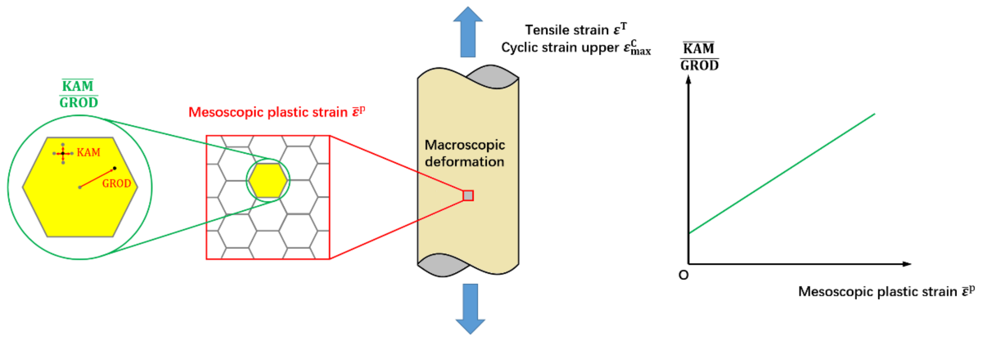
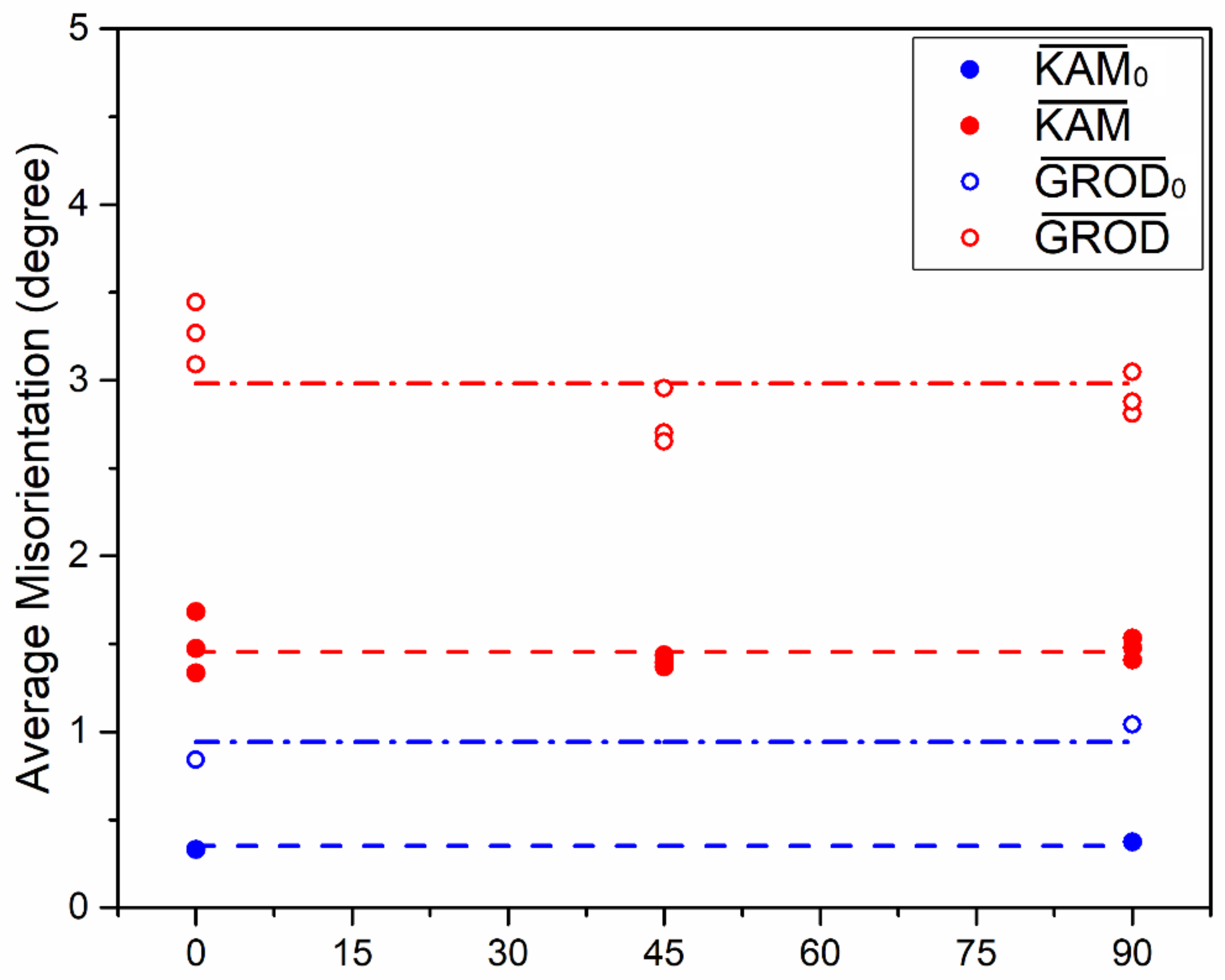
The average $\overline{KAM}$ and $\overline{GROD}$ values in the deformed gauge section measured on 2D-EBSD observational planes with different angles to loading axis are almost the same, which reveals the isotropic evolution law of $\overline{KAM}$ and $\overline{GROD}$ during the deformation.

(2)

Six fundamental assumptions including several necessary simplifications, such as spherical grain hypothesis and minimum activated slip factors number hypothesis, were made in this research to help us establish the modified 3D polycrystalline plasticity model based on our previous 2D model.

(3)

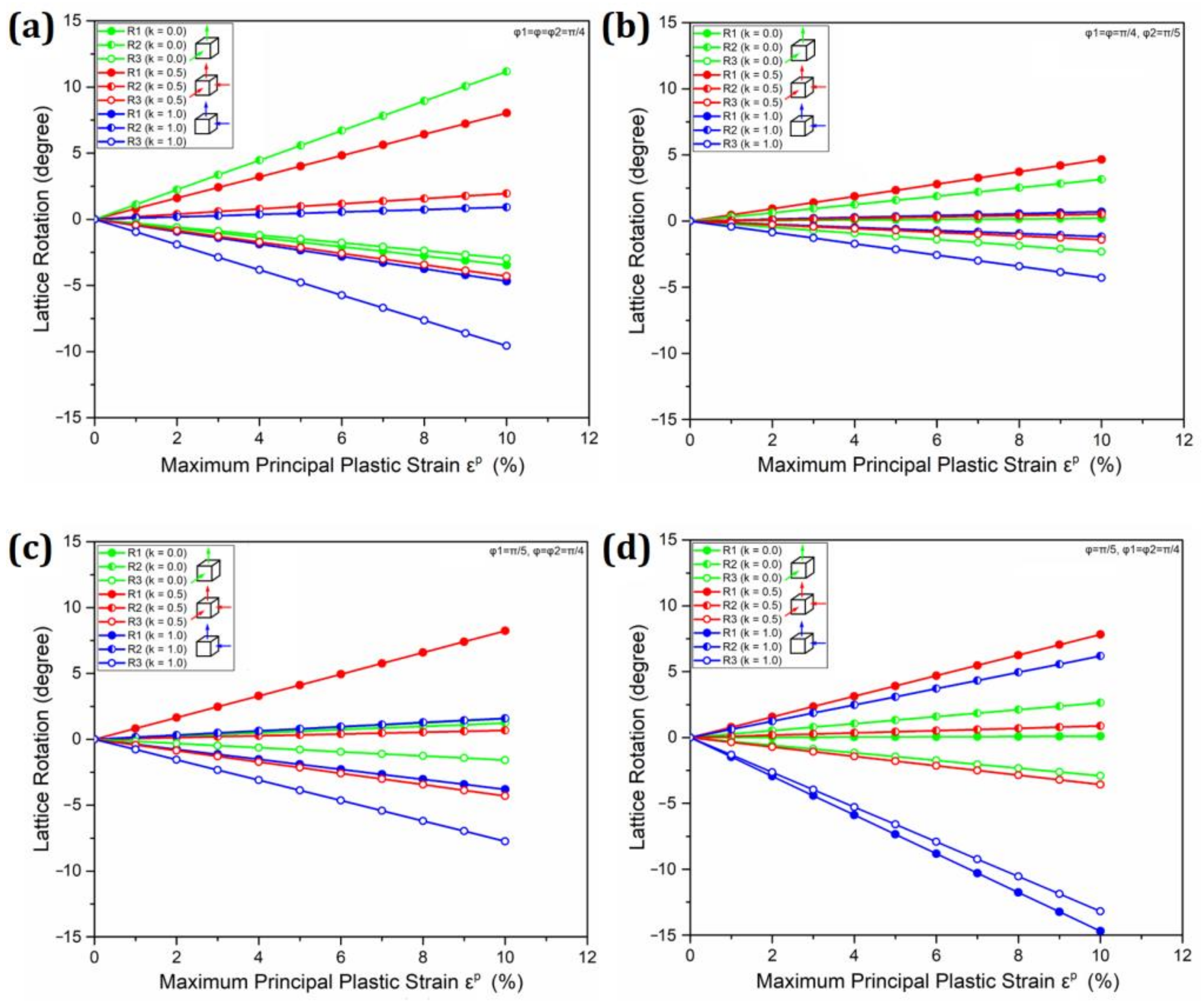
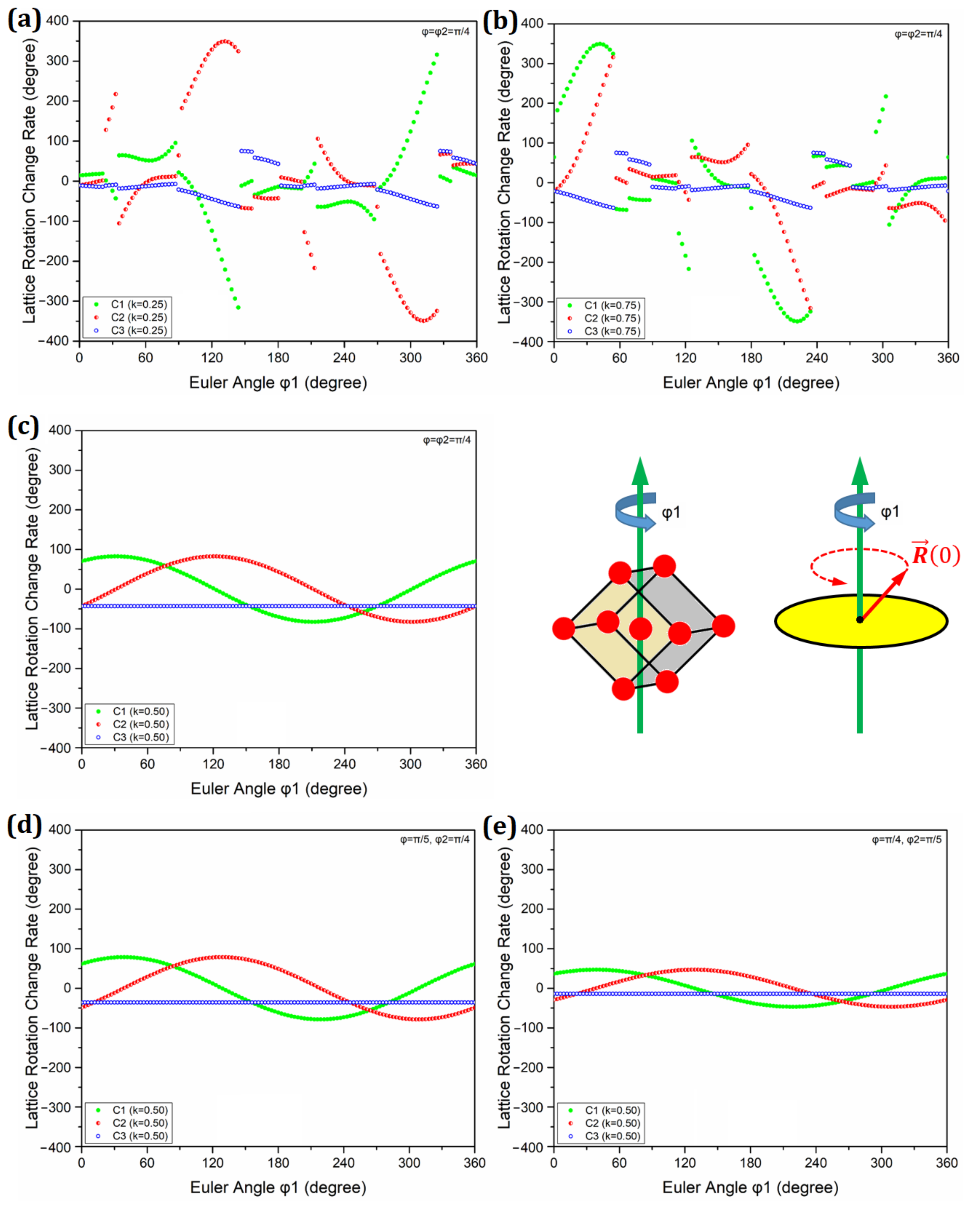
The relative lattice rotation $\overrightarrow{R}\left(0\right)$ at the GC and the intragranular misorientation distribution $\overrightarrow{R}\left(r\right)=\left(1-2r/D_{\mathrm{Grain}}\right)·\overrightarrow{\mathit{R}}\left(0\right)$ were calculated in different cases based on the equations given by the 3D polycrystalline plasticity model. The linear relationship $\left|\overrightarrow{\mathit{R}}\left(0\right)\right|=C\left(k, {\varphi }_1,\varphi ,{\varphi }_2\right)·{\epsilon }^{\mathrm{p}}$ turned out to exist between the relative lattice rotation angle $\left|\overrightarrow{\mathit{R}}\left(0\right)\right|$ at the GC and the maximum principal plastic strain ${\epsilon }^{\mathrm{p}}$ of RVE, where the coefficient C was influenced by both the Euler angles ${\varphi }_1,\varphi ,{\varphi }_2$ of any individual grain and the ratio k between another two principal plastic strains of RVE.

(4)

The $\overline{KAM}$ and $\overline{GROD}$ were theoretically derived from the intragranular misorientation distribution $\overrightarrow{\mathit{R}}\left(r\right)$ according to their definitions: $\overline{KAM}={\overline{C}}_f\left(k\right)·4a{\epsilon }^{\mathrm{p}}/\pi D_{\mathrm{Grain}}$ and $\overline{GROD}={\overline{C}}_{\mathit{g}}\left(k\right)·{\epsilon }^{\mathrm{p}}/3$. For polycrystalline metals with uniform equiaxial grains, ${\overline{C}}_f\left(k\right)$ and ${\overline{C}}_{\mathit{g}}\left(k\right)$ were turned out to be isotropic factors independent of 2D-EBSD observational plane selection. Therefore, both $\overline{KAM}$ and $\overline{GROD}$ follow the isotropic linear evolution law with the maximum principal plastic strain ${\epsilon }^{\mathrm{p}}$ and are meanwhile influenced by the ratio k between another two principal plastic strains of RVE.

(5)

Two laws given by this model were supported by experimental results: the linear evolution law of $\overline{KAM}$ and $\overline{GROD}$ has already been widely reported by previous studies, and the isotropic evolution law was verified by experimental result in this research.

References

- Brewer, L.N.; Field, D.P.; Merriman, C.C. Mapping and Assessing Plastic Deformation Using EBSD. In Electron Backscatter Diffraction in Materials Science, 2nd ed.; Schwartz, A.J., Kumar, M., Adams, B.L., Field, D.P., Eds.; Springer: Boston, MA, USA, 2009; pp. 251–262. [Google Scholar]
- Wright, S.I.; Nowell, M.M.; Field, D.P. A Review of Strain Analysis Using Electron Backscatter Diffraction. Microsc. Microanal. 2011, 17, 316–329. [Google Scholar] [CrossRef] [PubMed]
- Wright, S.I.; Suzuki, S.; Nowell, M.M. In Situ EBSD Observations of the Evolution in Crystallographic Orientation with Deformation. JOM 2016, 68, 2730–2736. [Google Scholar] [CrossRef]
- Kamaya, M. Measurement of local plastic strain distribution of stainless steel by electron backscatter diffraction. Mater. Charact. 2009, 60, 125–132. [Google Scholar] [CrossRef]
- Kamaya, M.; Wilkinson, A.J.; Titchmarsh, J.M. Measurement of plastic strain of polycrystalline material by electron backscatter diffraction. Nucl. Eng. Des. 2005, 235, 713–725. [Google Scholar] [CrossRef]
- Kamaya, M.; Wilkinson, A.J.; Titchmarsh, J.M. Quantification of plastic strain of stainless steel and nickel alloy by electron backscatter diffraction. Acta Mater. 2006, 54, 539–548. [Google Scholar] [CrossRef]
- Kamaya, M. Assessment of local deformation using EBSD: Quantification of accuracy of measurement and definition of local gradient. Ultramicroscopy 2011, 111, 1189–1199. [Google Scholar] [CrossRef]
- Kamaya, M.; da Fonseca, J.Q.; Li, L.M.; Preuss, M. Local Plastic Strain Measurement by EBSD. Appl. Mech. Mater. 2007, 7–8, 173–179. [Google Scholar] [CrossRef]
- Rui, S.-S.; Shang, Y.-B.; Su, Y.; Qiu, W.; Niu, L.-S.; Shi, H.-J.; Matsumoto, S.; Chuman, Y. EBSD analysis of cyclic load effect on final misorientation distribution of post-mortem low alloy steel: A new method for fatigue crack tip driving force prediction. Int. J. Fatigue 2018, 113, 264–276. [Google Scholar] [CrossRef]
- Rui, S.-S.; Shang, Y.-B.; Qiu, W.; Niu, L.-S.; Shi, H.-J.; Matsumoto, S.; Chuman, Y. Fracture mode identification of low alloy steels and cast irons by electron back-scattered diffraction misorientation analysis. J. Mater. Sci. Technol. 2017, 33, 1582–1595. [Google Scholar] [CrossRef]
- Kobayashi, D.; Miyabe, M.; Kagiya, Y.; Sugiura, R.; Yokobori, A.T. An Assessment and Estimation of the Damage Progression Behavior of IN738LC under Various Applied Stress Conditions Based on EBSD Analysis. Metall. Mater. Trans. A 2013, 44, 3123–3135. [Google Scholar] [CrossRef]
- Kobayashi, D.; Miyabe, M.; Achiwa, M. Failure Analysis and Life Assessment of Thermal Fatigue Crack Growth in a Nickel-Base Superalloy Based on EBSD Method. ASME Turbo Expo 2015, 2015, V006T21A004. [Google Scholar]
- Kobayashi, D.; Ito, A.; Miyabe, M.; Kagiya, Y.; Yoshioka, Y. Crack Initiation Behavior and its Estimation for a Gas Turbine Rotor Based on the EBSD Analysis. ASME Turbo Expo 2012, 2012, 71–79. [Google Scholar]
- Kobayashi, D.; Miyabe, M.; Achiwa, M. Failure Analysis Method of Ni-base Superalloy by EBSD Observation of the Cross Section. In Proceedings of the JSMS 13th Fractographic Conference, Wakayama, Japan, 14 November 2014. [Google Scholar]
- Kamaya, M. Characterization of microstructural damage due to low-cycle fatigue by EBSD observation. Mater. Charact. 2009, 60, 1454–1462. [Google Scholar] [CrossRef]
- Kamaya, M. Observation of Low-Cycle Fatigue Damage by EBSD(Microstructural Change in SUS316 and STS410). Trans. Jpn. Soc. Mech. Eng. 2011, 77, 154–169. [Google Scholar] [CrossRef] [Green Version]
- Kamaya, M.; Kuroda, M. Fatigue Damage Evaluation Using Electron Backscatter Diffraction. Mater. Trans. 2011, 52, 1168–1176. [Google Scholar] [CrossRef] [Green Version]
- Rui, S.-S.; Shang, Y.-B.; Fan, Y.-N.; Han, Q.-N.; Niu, L.-S.; Shi, H.-J.; Hashimoto, K.; Komai, N. EBSD analysis of creep deformation induced grain lattice distortion: A new method for creep damage evaluation of austenitic stainless steels. Mater. Sci. Eng. A 2018, 733, 329–337. [Google Scholar] [CrossRef]
- Kobayashi, D.; Miyabe, M.; Kagiya, Y.; Nagumo, Y.; Sugiura, R.; Matsuzaki, T.; Yokobori, A.T., Jr. Creep damage evaluation of IN738LC based on the EBSD method by using a notched specimen. Strength Fract. Complex. 2011, 7, 157–167. [Google Scholar] [CrossRef]
- Kobayashi, D.; Miyabe, M.; Kagiya, Y.; Nagumo, Y.; Sugiura, R.; Matsuzaki, T.; Yokobori, A.T. Geometrical influence for creep damage evaluation of IN738LC using electron backscatter diffraction. Mater. High Temp. 2012, 29, 301–307. [Google Scholar] [CrossRef]
- Wei, S.; Kim, J.; Tasan, C.C. Boundary micro-cracking in metastable Fe45Mn35Co10Cr10 high-entropy alloys. Acta Mater. 2019, 168, 76–86. [Google Scholar] [CrossRef]
- Han, Q.-N.; Rui, S.-S.; Qiu, W.; Ma, X.; Su, Y.; Cui, H.; Zhang, H.; Shi, H. Crystal orientation effect on fretting fatigue induced geometrically necessary dislocation distribution in Ni-based single-crystal superalloys. Acta Mater. 2019, 179, 129–141. [Google Scholar] [CrossRef]
- Kobayashi, D.; Takeuchi, T.; Achiwa, M. Evaluation of Fatigue Crack Growth Rate by the EBSD Method. In Proceedings of the JSME Annual Conference 2015, Tokyo, Japan, 13–16 September 2015. [Google Scholar]
- Jiang, J.; Britton, T.B.; Wilkinson, A.J. Measurement of geometrically necessary dislocation density with high resolution electron backscatter diffraction: Effects of detector binning and step size. Ultramicroscopy 2013, 125, 1–9. [Google Scholar] [CrossRef] [PubMed]
- Littlewood, P.D.; Wilkinson, A.J. Geometrically necessary dislocation density distributions in cyclically deformed Ti–6Al–4V. Acta Mater. 2012, 60, 5516–5525. [Google Scholar] [CrossRef]
- Wallis, D.; Hansen, L.N.; Britton, T.B.; Wilkinson, A.J. Geometrically necessary dislocation densities in olivine obtained using high-angular resolution electron backscatter diffraction. Ultramicroscopy 2016, 168, 34–45. [Google Scholar] [CrossRef] [PubMed] [Green Version]
- Jiang, J.; Britton, T.B.; Wilkinson, A.J. Evolution of dislocation density distributions in copper during tensile deformation. Acta Mater. 2013, 61, 7227–7239. [Google Scholar] [CrossRef]
- Wallis, D.; Hansen, L.N.; Britton, T.B.; Wilkinson, A.J. Dislocation Interactions in Olivine Revealed by HR-EBSD. J. Geophys. Res. Solid Earth 2017, 122, 7659–7678. [Google Scholar] [CrossRef] [Green Version]
- Vilalta-Clemente, A.; Naresh-Kumar, G.; Nouf-Allehiani, M.; Gamarra, P.; di Forte-Poisson, M.A.; Trager-Cowan, C.; Wilkinson, A.J. Cross-correlation based high resolution electron backscatter diffraction and electron channelling contrast imaging for strain mapping and dislocation distributions in InAlN thin films. Acta Mater. 2017, 125, 125–135. [Google Scholar] [CrossRef]
- Sarac, A.; Oztop, M.S.; Dahlberg, C.F.O.; Kysar, J.W. Spatial distribution of the net Burgers vector density in a deformed single crystal. Int. J. Plast. 2016, 85, 110–129. [Google Scholar] [CrossRef] [Green Version]
- Kysar, J.W.; Gan, Y.X.; Morse, T.L.; Chen, X.; Jones, M.E. High strain gradient plasticity associated with wedge indentation into face-centered cubic single crystals: Geometrically necessary dislocation densities. J. Mech. Phys. Solids 2007, 55, 1554–1573. [Google Scholar] [CrossRef]
- Dahlberg, C.F.O.; Saito, Y.; Öztop, M.S.; Kysar, J.W. Geometrically necessary dislocation density measurements at a grain boundary due to wedge indentation into an aluminum bicrystal. J. Mech. Phys. Solids 2017, 105 (Suppl. C), 131–149. [Google Scholar] [CrossRef]
- Dahlberg, C.F.O.; Saito, Y.; Öztop, M.S.; Kysar, J.W. Geometrically necessary dislocation density measurements associated with different angles of indentations. Int. J. Plast. 2014, 54, 81–95. [Google Scholar] [CrossRef]
- Sarac, A.; Kysar, J.W. Experimental validation of plastic constitutive hardening relationship based upon the direction of the Net Burgers Density Vector. J. Mech. Phys. Solids 2018, 111 (Suppl. C), 358–374. [Google Scholar] [CrossRef]
- Kysar, J.W.; Saito, Y.; Oztop, M.S.; Lee, D.; Huh, W.T. Experimental lower bounds on geometrically necessary dislocation density. Int. J. Plast. 2010, 26, 1097–1123. [Google Scholar] [CrossRef]
- Pantleon, W. Resolving the geometrically necessary dislocation content by conventional electron backscattering diffraction. Scr. Mater. 2008, 58, 994–997. [Google Scholar] [CrossRef]
- Calcagnotto, M.; Ponge, D.; Demir, E.; Raabe, D. Orientation gradients and geometrically necessary dislocations in ultrafine grained dual-phase steels studied by 2D and 3D EBSD. Mater. Sci. Eng. A 2010, 527, 2738–2746. [Google Scholar] [CrossRef]
- Konijnenberg, P.J.; Zaefferer, S.; Raabe, D. Assessment of geometrically necessary dislocation levels derived by 3D EBSD. Acta Mater. 2015, 99, 402–414. [Google Scholar] [CrossRef]
- Gao, H.; Huang, Y. Geometrically necessary dislocation and size-dependent plasticity. Scr. Mater. 2003, 48, 113–118. [Google Scholar] [CrossRef]
- Arsenlis, A.; Parks, D.M. Crystallographic aspects of geometrically-necessary and statistically-stored dislocation density. Acta Mater. 1999, 47, 1597–1611. [Google Scholar] [CrossRef]
- Nye, J.F. Some geometrical relations in dislocated crystals. Acta Metall. 1953, 1, 153–162. [Google Scholar] [CrossRef]
- Bilby, B.A.; Bullough, R.; Smith, E. Continuous distributions of dislocations: A new application of the methods of non-Riemannian geometry. Proc. R. Soc. Lond. Ser. A. Math. Phys. Sci. 1955, 231, 263. [Google Scholar]
- Kröner, E. Continuum Theory of Dislocation and Self-Stresses; Springer: Berlin, Germany, 1958. [Google Scholar]
- Harte, A.; Atkinson, M.; Preuss, M.; da Fonseca, J.Q. A statistical study of the relationship between plastic strain and lattice misorientation on the surface of a deformed Ni-based superalloy. Acta Mater. 2020, 195, 555–570. [Google Scholar] [CrossRef]
- Rui, S.-S.; Niu, L.-S.; Shi, H.-J.; Wei, S.; Tasan, C.C. Diffraction-based misorientation mapping: A continuum mechanics description. J. Mech. Phys. Solids 2019, 133, 103709. [Google Scholar] [CrossRef]
- Hutchinson, J.W.; Neale, K.W. Finite Strain J2 Deformation Theory. In Proceedings of the IUTAM Symposium on Finite Elasticity; Carlson, D.E., Shield, R.T., Eds.; Springer: Dordrecht, The Netherlands, 1982; pp. 237–247. [Google Scholar]
- Standard Test Methods for Tension Testing of Metallic Materials; ASTM International: West Conshohocken, PA, USA, 2008.
- Han, Q.-N.; Rui, S.-S.; Qiu, W.; Su, Y.; Ma, X.; Su, Z.; Cui, H.; Shi, H. Effect of crystal orientation on the indentation behaviour of Ni-based single crystal superalloy. Mater. Sci. Eng. A 2020, 773, 138893. [Google Scholar] [CrossRef]
- Cho, J.-H.; Rollett, A.D.; Oh, K.H. Determination of a mean orientation in electron backscatter diffraction measurements. Metall. Mater. Trans. A 2005, 36, 3427–3438. [Google Scholar] [CrossRef]
- Glez, J.C.; Driver, J. Orientation distribution analysis in deformed grains. J. Appl. Crystallogr. 2001, 34, 280–288. [Google Scholar] [CrossRef]
- Ashby, M.F. The deformation of plastically non-homogeneous materials. Philos. Mag. 1970, 21, 399–424. [Google Scholar] [CrossRef]
- Kundu, A.; Field, D.P. Influence of plastic deformation heterogeneity on development of geometrically necessary dislocation density in dual phase steel. Mater. Sci. Eng. A 2016, 667, 435–443. [Google Scholar] [CrossRef]