
A Tool for Rapid Analysis Using Image Processing and Artificial Intelligence: Automated Interoperable Characterization Data of Metal Powder for Additive Manufacturing with SEM Case
 , and
, and
Abstract
:1. Introduction
1.1. Applications on Additive Manufacturing
1.2. Relevant Work—SotA
1.3. AI and Computer Vision
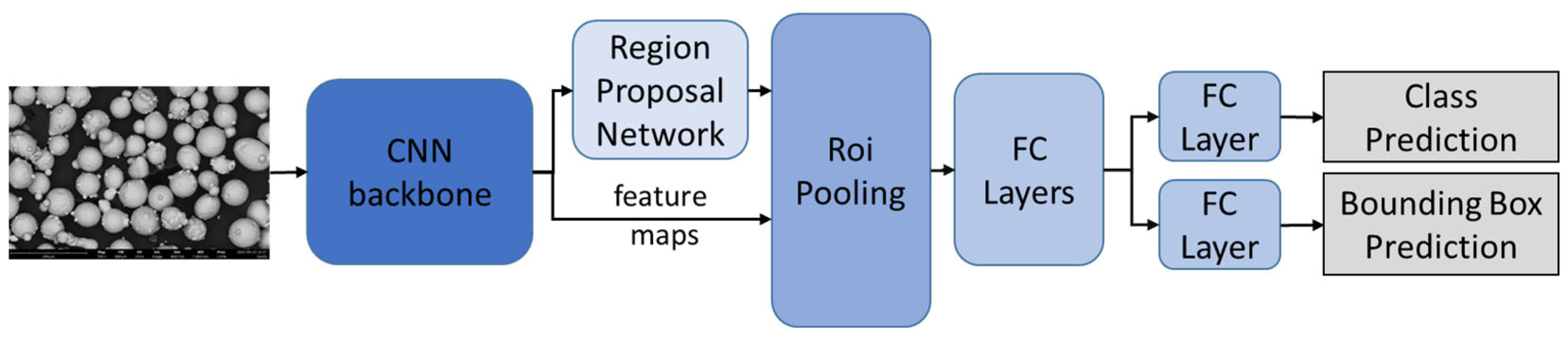
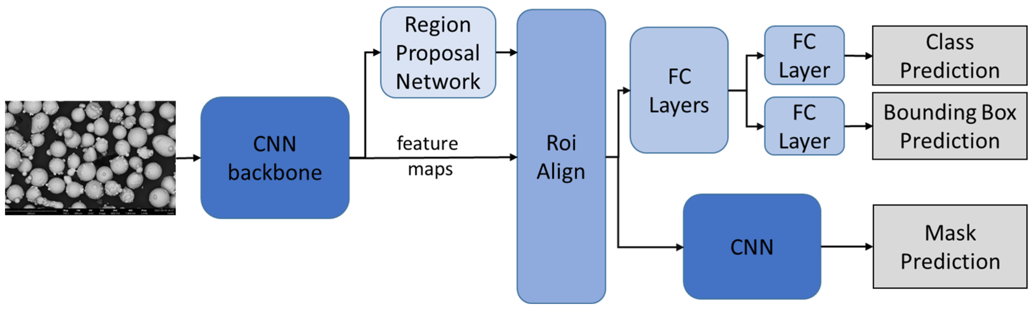
1.4. Mask R-CNN and Previous Models
1.5. Semantic Segmentation
1.6. Problem Description
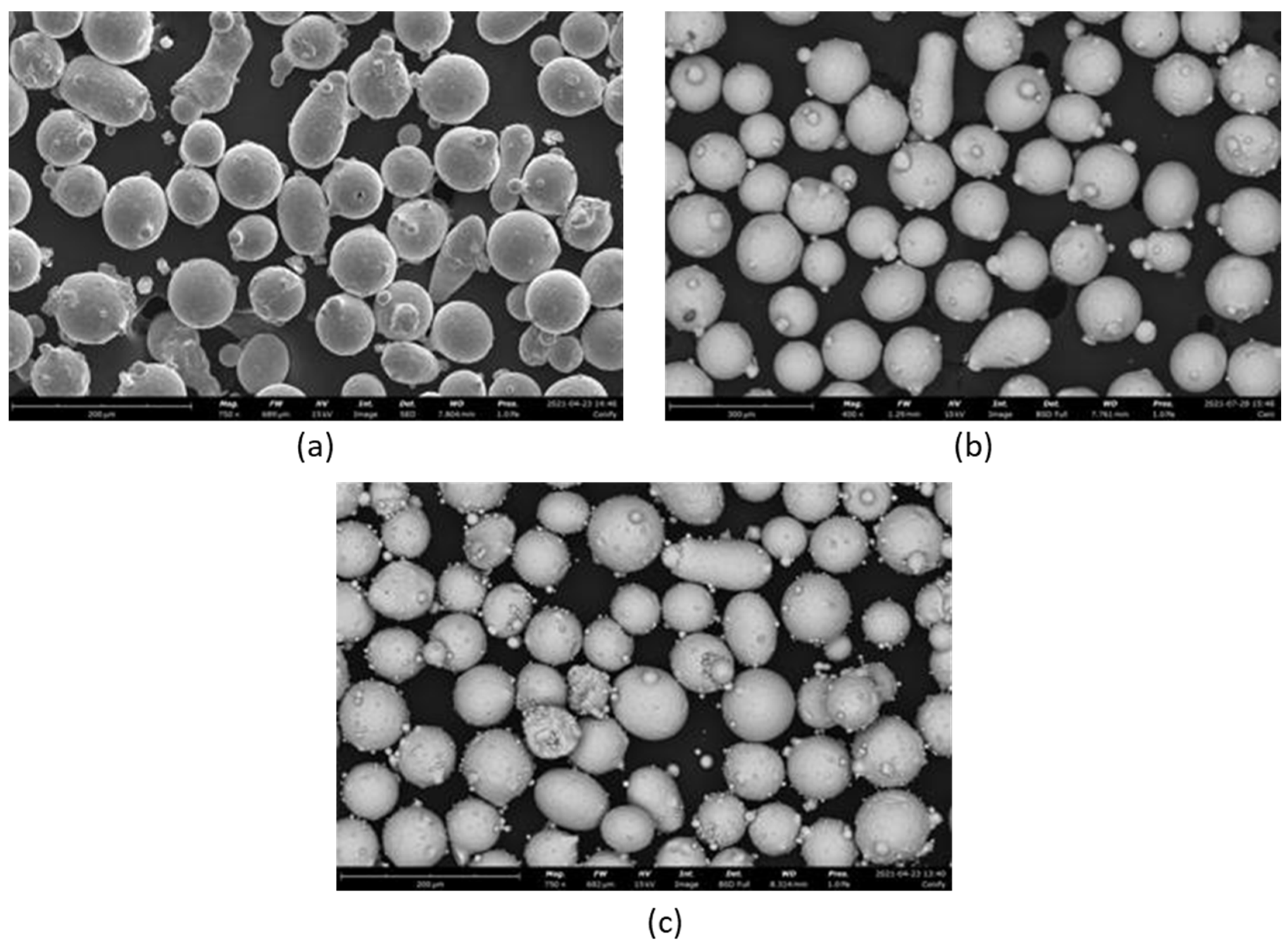
2. Materials and Methods
2.1. Training and Methodology
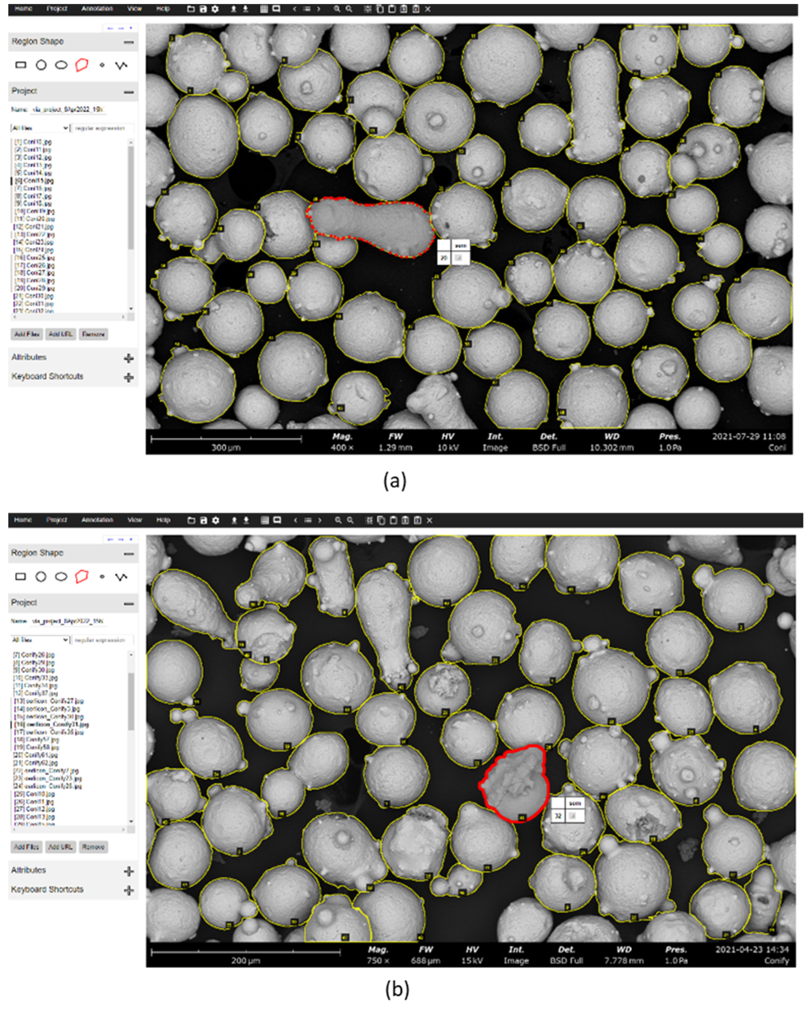
Annotation Labels
2.2. Training
- -
- Horizontal flip
- -
- Vertical flip
- -
- Rotation of [0, 90, 180, 270] angle
- -
- Random brightness with intensity in (0.9, 1.1)
- -
- Random contrast with intensity in (0.9, 1.1)
- -
- Random saturation with intensity in (0.9, 1.1)
- -
- Random lighting with standard deviation of principal component weighting equal to 0.9
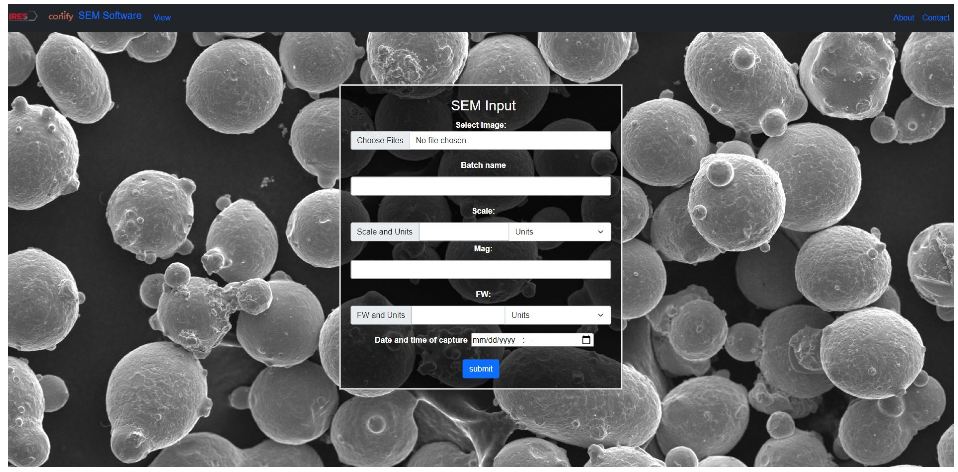
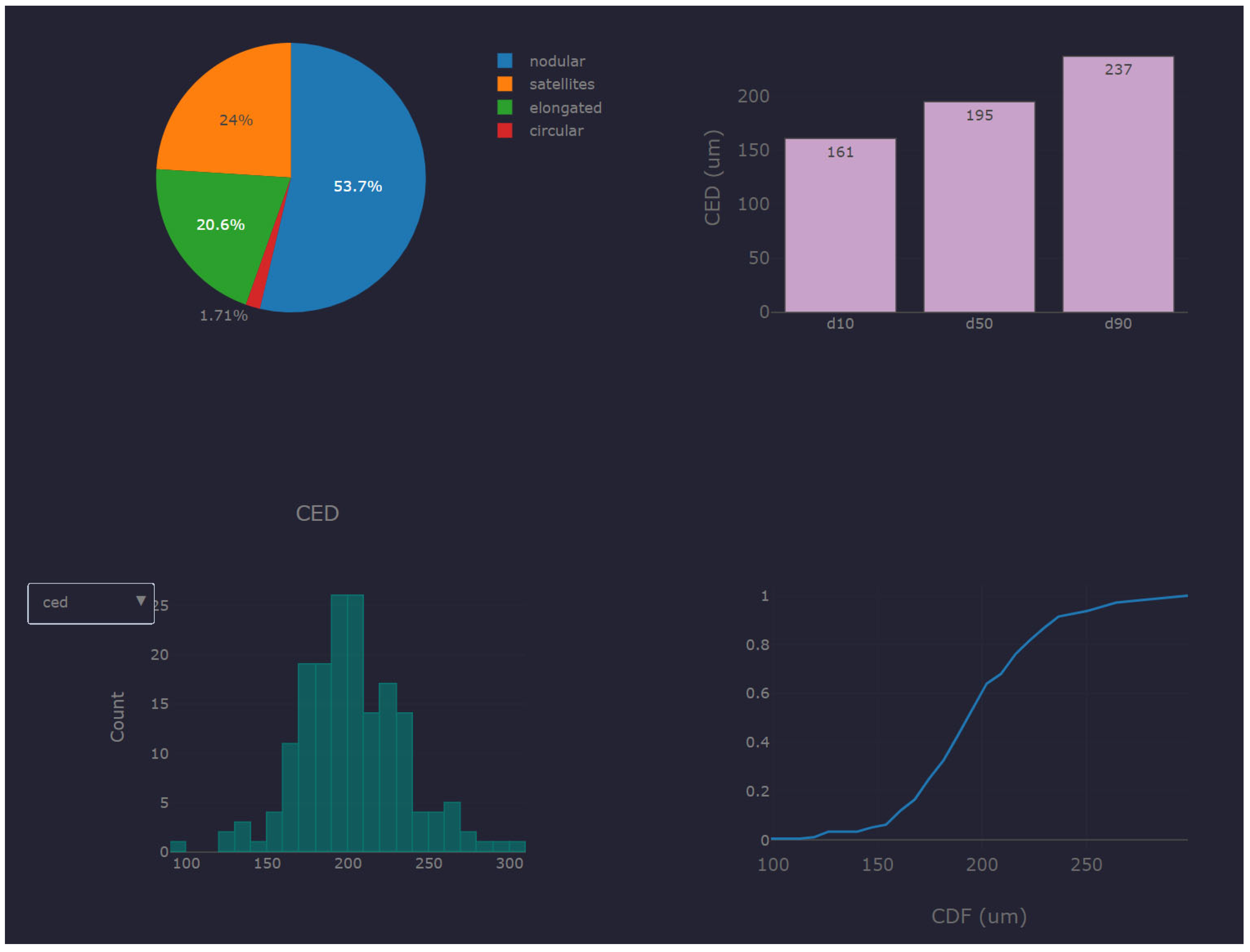
2.3. Framework—Software
3. Results and Discussion
3.1. Trained Mask R-CNN Model Metrics
- True positive (TP) is when a prediction–target mask (and label) pair has an IoU score which exceeds a predefined threshold.
- False positive (FP) indicates a predicted object mask that has no associated ground truth object mask.
- False negative (FN) indicates a ground truth object mask that has no associated predicted object mask.
- True negative (TN) is the background region correctly not being detected by the model, these regions are not explicitly annotated in an instance segmentation problem. Thus, we chose not to calculate it.
- Accuracy =
- Precision =
- AP50 = , for n classes
3.2. Discussion
4. Conclusions & Future Work
Author Contributions
Funding
Institutional Review Board Statement
Informed Consent Statement
Data Availability Statement
Conflicts of Interest
References
- Slotwinski, J.A.; Garboczi, E.J.; Stutzman, P.; Ferraris, C.; Watson, S.; Peltz, M. Characterization of Metal Powders Used for Additive Manufacturing. J. Res. Natl. Inst. Stand. Technol. 2014, 119, 460–493. [Google Scholar] [CrossRef] [PubMed]
- Binayak, B. Comparative Study of Popular Deep Learning Models for Machining Roughness Classification Using Sound and Force Signals. Micromachines 2021, 12, 1484. [Google Scholar]
- Binayak, B.; GiJun, P. Non-contact surface roughness evaluation of milling surface using CNN-deep learning models. Int. J. Comput. Integr. Manuf. 2022, 1–15. [Google Scholar] [CrossRef]
- DeCost, B.; Jain, H.; Rollett, A.; Holm, E. Computer Vision and Machine Learning for Autonomous Characterization of AM Powder Feedstocks. JOM 2016, 69, 456. [Google Scholar] [CrossRef] [Green Version]
- Zhou, X.; Dai, N.; Cheng, X.; Thompson, A.; Leach, R. Intelligent classification for three-dimensional metal powder particles. Powder Technol. 2022, 397, 117018. [Google Scholar] [CrossRef]
- Kirillov, A.; Wu, Y.; He, K.; Girshick, R. PointRend: Image Segmentation as Rendering. arXiv 2019, arXiv:1912.08193. [Google Scholar]
- Cohn, R.; Anderson, I.; Prost, T.; Tiarks, J.; White, E.; Holm, E. Instance Segmentation for Direct Measurements of Satellites in Metal Powders and Automated Microstructural Characterization from Image Data. JOM 2021, 73, 2159–2172. [Google Scholar] [CrossRef]
- Chai, J.Z. Deep learning in computer vision: A critical review of emerging techniques and application scenarios. Mach. Learn. Appl. 2021, 6, 100134. [Google Scholar] [CrossRef]
- Girshick, R.; Donahue, J.; Darrell, T.; Malik, J. Region-Based Convolutional Networks for Accurate Object Detection and Segmentation. IEEE Trans. Pattern Anal. Mach. Intell. 2015, 38, 142–158. [Google Scholar] [CrossRef]
- Ren, S.; He, K.; Girshick, R.; Sun, J. Faster R-CNN: Towards Real-Time Object Detection with Region Proposal Networks. arXiv 2015, arXiv:2016.2577031. [Google Scholar]
- He, K.; Gkioxari, G.; Dollár, P.; Girshick, R. Mask R-CNN. In Proceedings of the 2017 IEEE International Conference on Computer Vision (ICCV), Venice, Italy, 22–29 October 2007; pp. 2961–2969. [Google Scholar] [CrossRef]
- Zhang, A.; Lipton, Z.C.; Li, M.; Smola, A.J. Dive into Deep Learning. arXiv 2021, arXiv:2106.11342. [Google Scholar]
- Thomas, M.; Drawin, S. Role of Metal Powder Characteristics in Additive Manufacturing. In Proceedings of the PM2016 World Congress, Hamburg, Germany, 9–13 October 2016. [Google Scholar]
- Van Rossum, G.; Drake, F.L., Jr. Python Reference Manual; Centrum Voor Wiskunde en Informatica: Amsterdam, The Netherlands, 1995. [Google Scholar]
- Ren, P.; Xiao, Y.; Chang, X.; Huang, P.-Y.; Li, Z.; Gupta, B.B.; Wang, X. A Survey of Deep Active Learning. arXiv 2020, arXiv:2009.00236. [Google Scholar]
- Wu, Y.; Kirillov, A.; Massa, F.; Lo, W.-Y.; Girshick, R. Detectron2 Open Source Repository. 2019. Available online: https://github.com/facebookresearch/detectron2 (accessed on 1 October 2022).
- Paszke, A.; Gross, S.; Massa, F.; Lerer, A.; Bradbury, J.; Chanan, G.; Chintala, S.; PyTorch: An Imperative Style, High-Performance Deep Learning Library. In Advances in Neural Information Processing Systems 32; Wallach, H., Larochelle, H., Beygelzimer, A., Alché-Buc, F., Fox, E., Garnett, R., Eds.; 2019. Available online: http://papers.neurips.cc/paper/9015-pytorch-an-imperative-style-high-performance-deep-learning-library.pdf (accessed on 1 October 2022).
- Dutta, A.; Zisserman, A. The VIA Annotation Software for Images, Audio and Video. In Proceedings of the 27th ACM International Conference on Multimedia 2019, Nice, France, 21–25 October 2019; pp. 2276–2279. [Google Scholar] [CrossRef] [Green Version]
- Lin, T.-Y.; Dollár, P.; Girshick, R.; He, K.; Hariharan, B.; Belongie, S. Feature Pyramid Networks for Object Detection. arXiv 2016, arXiv:1612.03144. [Google Scholar]
- He, K.; Zhang, X.; Ren, S.; Sun, J. Deep Residual Learning for Image Recognition. arXiv 2015, arXiv:1512.03385. [Google Scholar]
- Lin, T.-Y.; Maire, M.; Belongie, S.; Bourdev, L.; Girshick, R.; Hays, J.; Dollár, P. Microsoft COCO: Common Objects in Context. arXiv 2014, arXiv:1405.0312. [Google Scholar]
- Loshchilov, I.; Hutter, F. Decoupled Weight Decay Regularization. arXiv 2017, arXiv:1711.05101. [Google Scholar]
- Smith, L.N. Cyclical Learning Rates for Training Neural Networks. arXiv 2015, arXiv:1506.01186. [Google Scholar]
- Snoek, J.; Larochelle, H.; Adams, R.P. Practical Bayesian Optimization of Machine Learning Algorithms. arXiv 2012, arXiv:1206.2944. [Google Scholar]
- Biewald, L. Experiment Tracking with Weights and Biases. 2020. Available online: https://www.wandb.com/ (accessed on 1 October 2022).
- Grinberg, M. Flask Web Development: Developing Web Applications with Python; O’Reilly Media, Inc.: Sebastopol, CA, USA, 2018. [Google Scholar]
- Shanbhag, G.; Vlasea, M. Powder Reuse Cycles in Electron Beam Powder Bed Fusion—Variation of Powder Characteristics. Materials 2021, 14, 4602. [Google Scholar] [CrossRef]
- Arase, K.M. Rethinking Task and Metrics of Instance Segmentation on 3D Point Clouds. In Proceedings of the IEEE/CVF International Conference on Computer Vision Workshop, Seoul, Korea, 27–28 October 2019. [Google Scholar]
- Yang, F.Y. Accurate Instance Segmentation for Remote Sensing Images via Adaptive and Dynamic Feature Learning. Remote Sens. 2021, 13, 4774. [Google Scholar] [CrossRef]
- Schneider, C.A.; Rasband, W.S.; Eliceiri, K.W. NIH Image to ImageJ: 25 years of image analysis. Nat. Methods 2012, 9, 671–675. [Google Scholar] [CrossRef] [PubMed]


| Brand Name | Chemical Composition (wt. %) | Production Process | PSD (Nominal Range) | Apparent Density | Morphology | ||||||
|---|---|---|---|---|---|---|---|---|---|---|---|
| Fe | Cr | Mo | Si | V | Mn | C | |||||
| Oerlikon Metco H13 | Balance | 5.2 | 1.3 | 1.0 | 1.0 | - | 0.4 | Gas Atomization | 45–90 μm | >4.0 g/cm3 | Spheroidal |
| GKN Additive H13 | Balance | 5.2 | 1.3 | 0.8 | 1.2 | 0.3 | 0.4 | Gas Atomization | 50–150 μm | - | Spheroidal |
| Atomizing H13 | Balance | 5.2 | 1.3 | 0.8 | 1.2 | 0.3 | 0.4 | Gas Atomization | 45–90 μm | - | Spheroidal |
| Type of Structure | Category |
|---|---|
| Particles with Satellites | Satellites |
| Nodular Particles (Agglomerated and Splat Cap) | Nodular |
| Elongated Particles | Elongated |
| Circular Particles | Circular |
| Category | Annotated Label Instances |
|---|---|
| Satellites | 1614 |
| Nodular | 1109 |
| Elongated | 377 |
| Circular | 422 |
| Category | Value | Description |
|---|---|---|
| GPU_COUNT | 1 | Number of GPUs utilized for training |
| BATCH SIZE | 2 | Number of images on one train step |
| NUM_CLASSES | 4 | Number of classes |
| EPOCHS | 53 | Number of training passes utilizing the whole dataset |
| LEARNING_RATE | 10−4 | Maximum value of learning rate |
| WEIGHT_DECAY | 10−5 | Weight decay regularization |
| TRAIN_ROIS_PER_IMAGE | 256 | Number of ROIs per image to feed to classifier/mask heads |
| RPN_NMS_THRESHOLD | 0.7 | Non-maximum suppression threshold of region proposal network |
| ROI_NMS_THRESHOLD | 0.65 | Non-maximum suppression threshold of region of interest heads |
| DETECTION_MIN_ CONFIDENCE | 0.45 | Minimum probability value to accept a detected instance |
| IMAGE_MIN_DIM | 1000 | Resized image minimum size |
| IMAGE_MAX_DIM | 1333 | Resized image maximum size |
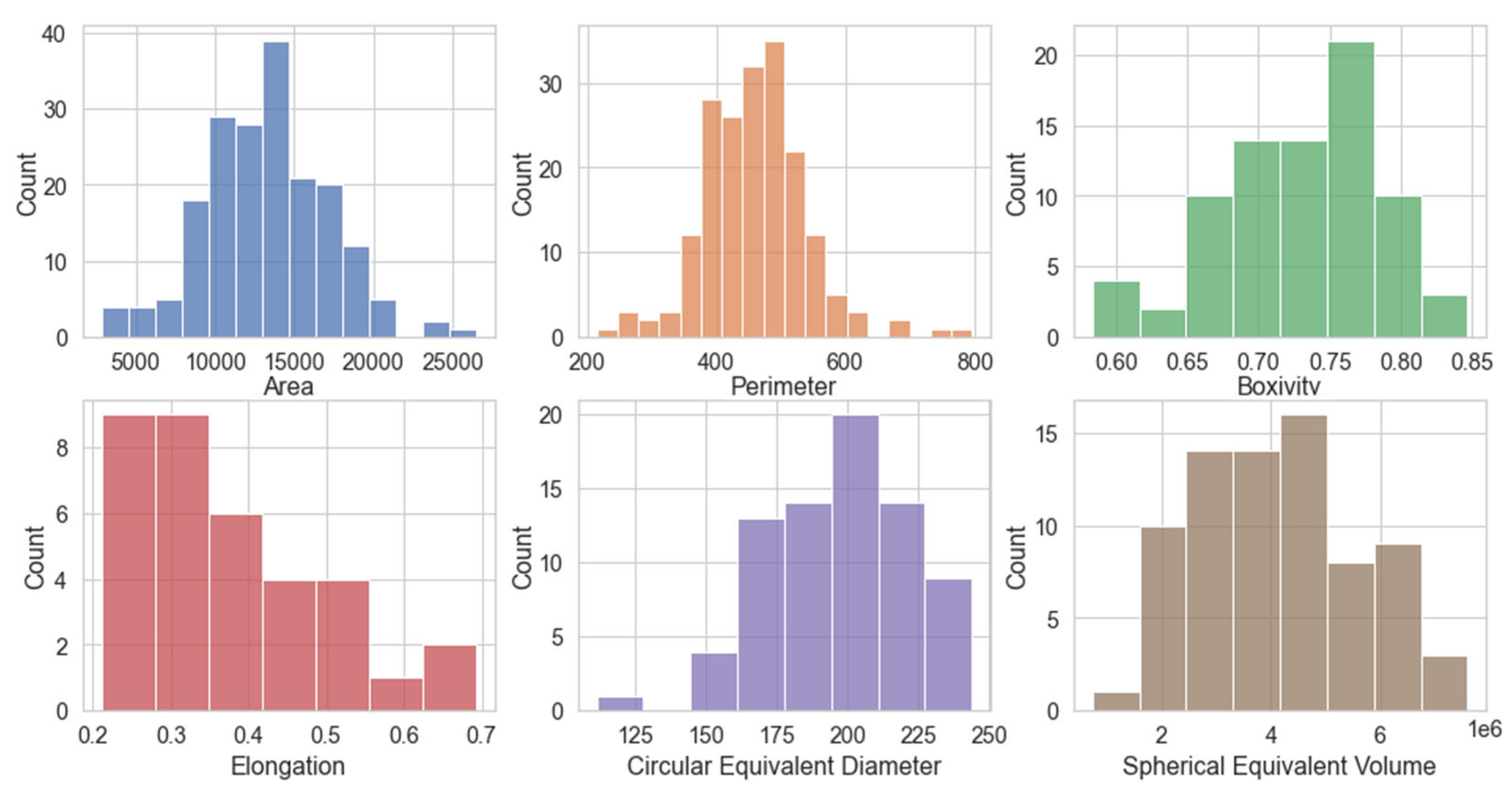
| Property | Symbol | Equation | Applied Particle Type | Units |
|---|---|---|---|---|
| Area | A | All | (nm2 or μm2) | |
| Perimeter | P | All | (nm or μm) | |
| Elongation | E | Elongated | [0, 1] | |
| Boxivity | B | Nodular | [0, 1] | |
| Circular Equivalent Diameter | χA | Circular, Satellites | (nm or μm) | |
| Spherical Equivalent Volume | V | Circular, Satellites | (nm3 or μm3) |
| Loss Type | Train Value | Validation Value |
|---|---|---|
| Total Loss | 0.325 | 0.789 |
| Class Loss | 0.169 | 0.410 |
| Bounding box Loss | 0.069 | 0.168 |
| Mask Loss | 0.047 | 0.114 |
| Dataset | AP50 |
|---|---|
| Overall | 67.2 |
| Elongated | 69.5 |
| Satellites | 74.5 |
| Circular | 57.2 |
| Nodular | 60.7 |
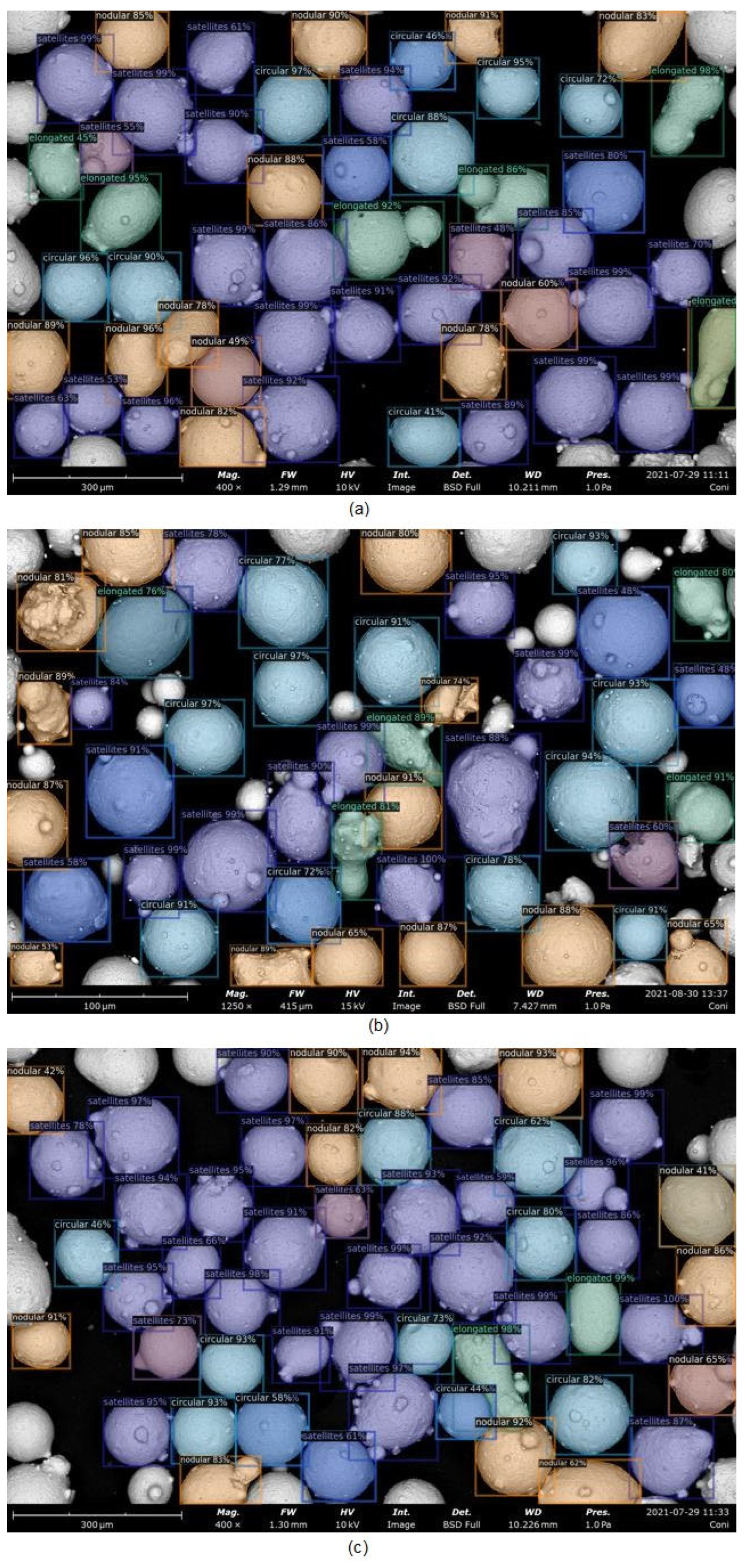
| Particle Type | Color Coding |
|---|---|
| Elongated | |
| Satellites | |
| Circular | |
| Nodular |
Publisher’s Note: MDPI stays neutral with regard to jurisdictional claims in published maps and institutional affiliations. |
© 2022 by the authors. Licensee MDPI, Basel, Switzerland. This article is an open access article distributed under the terms and conditions of the Creative Commons Attribution (CC BY) license (https://creativecommons.org/licenses/by/4.0/).
Share and Cite
Bakas, G.; Dimitriadis, S.; Deligiannis, S.; Gargalis, L.; Skaltsas, I.; Bei, K.; Karaxi, E.; Koumoulos, E.P. A Tool for Rapid Analysis Using Image Processing and Artificial Intelligence: Automated Interoperable Characterization Data of Metal Powder for Additive Manufacturing with SEM Case. Metals 2022, 12, 1816. https://doi.org/10.3390/met12111816
Bakas G, Dimitriadis S, Deligiannis S, Gargalis L, Skaltsas I, Bei K, Karaxi E, Koumoulos EP. A Tool for Rapid Analysis Using Image Processing and Artificial Intelligence: Automated Interoperable Characterization Data of Metal Powder for Additive Manufacturing with SEM Case. Metals. 2022; 12(11):1816. https://doi.org/10.3390/met12111816
Chicago/Turabian StyleBakas, Georgios, Spyridon Dimitriadis, Stavros Deligiannis, Leonidas Gargalis, Ioannis Skaltsas, Kyriaki Bei, Evangelia Karaxi, and Elias P. Koumoulos. 2022. "A Tool for Rapid Analysis Using Image Processing and Artificial Intelligence: Automated Interoperable Characterization Data of Metal Powder for Additive Manufacturing with SEM Case" Metals 12, no. 11: 1816. https://doi.org/10.3390/met12111816