Corrosion Behavior of L245N Standard Steel in CO₂ Saturated Brine under Flow Condition

Abstract

The corrosion behavior of oilfield used L245N standard steel was tested in simulated oilfield solution by dynamic high-temperature autoclave. The corrosion products were characterized by using scanning electron microscopy (SEM), X-ray diffraction (XRD) and Electrochemical impedance spectroscopy (EIS) respectively. In addition, the corrosion rates and surface morphological characteristics of the steels after different exposure times were studied. The results showed that the corrosion rate decreased sharply and then increased with time in the high salinity flow solution, which was related to the formation of corrosion scale and the remaining cementite within it. At the beginning of the exposure time, the formed corrosion scale became thicker, resulting in a significant decrease of the corrosion rate. While with increasing time, on the one hand, the increased remaining cementite within corrosion scale facilitated the corrosion by the galvanic corrosion between the remaining cementite and the ferrite within the metal. On the other hand, the protective effect of corrosion scale formed on the remaining cementite skeleton declined due to the formation of large amounts of Fe_xCa_1−xCO₃, which also promoted the corrosion rate of the steels, both these ways contributed to a slow increase of corrosion rate.

1. Introduction

20# carbon steel has been widely used as the oilfield pipeline material. The designed service life of these oilfield pipelines should be 5–8 years. However, it actually decreases to less than 4 years due to oil leakage accidents driven by serious pipeline corrosion [1,2], which causes significant environmental damage and economic losses [3,4]. To improve the oil recovery rate, oilfield produced water has been injected into the oil field when products begin [5,6]. However, the contents of H₂S, CO₂, inorganic ions and bacteria increased with the increasing composite water cut [6]. The high oilfield brine easily caused perforation by serious corrosion of the carbon steel [4].

In recent years, many researchers have tried to investigate the mechanism and factors of the CO₂ corrosion. It is considered that the scales of mineralized ions formed a relatively occluded microenvironment, and the presence of CO₂ accelerated the deterioration of the environment within the occluded corrosion micro-battery and accelerated the perforation rate [7,8]. The effect of chloride concentration on the CO₂ corrosion have been studied; some reports regarded that the pitting corrosion was related to the high chloride concentration [9,10]. However, other reports also found that pitting corrosion was not observed at any salt concentration, and that the corrosion rate decreased with increasing salt concentrations [11]. The oil content also affected the corrosion of carbon steel, because the existence of oil phase was beneficial to the cathodic partial to promote the corrosion process [12]. Mansoori et al. [13,14] observed that different concentrations of Ca²⁺ and Mg²⁺ ions could act as key factors in general, and localized corrosion with different exposure times by influencing the nucleation/precipitation of FeCO₃ and Fe_xCa_1−xCO₃ within Fe₃C pores. The loose corrosion scale formed by the effect of Ca²⁺ ions decreased the protective effect and increased the corrosion rate [15,16]. However, when the concentration of Ca²⁺ was high enough, the corrosion rate would not decrease [17].

The microstructure also plays a significant role in terms of the corrosion rate and mechanism [18,19,20] and the inhibitor efficiency [21,22,23]. Mishra et al. established an empirical relationship between carbon steel corrosion and microstructure [24,25]. The inhomogeneity of microstructure in steel, such as grain boundaries, pearlitic colonies and banded phases, resulted in the acceleration of local anodic dissolution [26]. Meanwhile, it has been reported that the retained austenite in steel significantly resisted corrosion due to low residual stresses [27,28,29,30]. The effect of Fe₃C on the corrosion process of carbon steel has been studied. The corrosion could be promoted by the enhanced galvanic effect between the remaining cementite and ferrite in the matrix [31]. Mora–Mendoza et al. observed that the Fe₃C layer in the corrosion film caused a cathodic area increase, leading to the corrosion rate increase with time [32]. Moreover, the effect of Fe₃C under flow condition has also been reported; Fe₃C could anchor the corrosion film to resist turbulent flow [33], but for the conditions where it is difficult to form a protective film, Fe₃C instead aggravated the corrosion process [34].

However, the study about the corrosion process in solution containing Ca²⁺ under flow condition was barely reported. The effect of Ca²⁺ ions and the remaining cementite on the corrosion mechanism in the flow environment is not fully understood. The present work aims to investigate the corrosion behavior of carbon steel in simulated flow oilfield water. The corrosion scale and metal surface morphology evolution were evaluated by SEM, XRD, EIS and a white light interferometer.

2. Materials and Methods

2.1. Materials and Solution Environment

20# carbon steel used in this work was manufactured following the Chinese standard GB/T 9711-2011 (L245N), which is widely referred to in the petrochemical industry. GB/T 9711-2011 (L245N) requires normalizing rolling for grain refining [35]. The elemental compositions of L245N standard steel are given in

Table 1. The elemental compositions of L245N standard steel, (wt. %).

Standard	C	Si	Mn	Cr	P	S	Cu	Fe
L245N	0.20	0.30	0.45	0.012	0.013	0.018	0.011	Bal.

.

2.2. Rotary Coupon Test

A dynamic high temperature autoclave (FCZ5-20, DL Kemao Test Equipment Co., Ltd., Dalian, China) was used for rotary coupon test in this work. Considering the circular motion of testing samples in the autoclave, arc-shaped specimens were machined from L245N standard steel. If the sample surface was flat, the velocity of the fluid flowing through the sample surface would be nonuniform, and that would affect the corrosion test. Figure 1 shows the dimensions of the specimen. The outside curved surface with a width of 12 mm was the experimental surface, and other surfaces covered with silica gel were non-experimental areas without contact with the experiment solution. The corrosion scales formed on the specimens after 1/2 day, 2, 4 and 7 days corrosion test in the autoclave was measured by scanning electron microscopy (SEM; JEOL Ltd., Tokyo, Japan), energy dispersive spectroscopy (EDS) and XRD (M21X, MACSCIENCECO, Ltd., Tokyo, Japan), respectively. Finally, the corrosion products were removed to obtain the corrosion rates, and the surface morphologies after descaling were characterized by a white light interferometer (Bruker Surface Profiler, Contour GT-K1, Bruker Nano, Inc., Tucson, AZ, USA).

The sample surface of the arc-shaped specimen was grinded step by step with 360, 600, 800, 1000, 1500, and 2000 # abrasive papers and polished with corundum powders of 2.5 μm in diameter. It was then immersed into distilled water to clean and defat with ethanol and acetone, and at last weighed after cold air drying.

Before the experiments, 99.95% high purity nitrogen was first bubbled into the corrosion medium for 2 h to remove oxygen. The solution was the oilfield produced water simulation fluid as shown in

Table 2. Composition of the experiment solution.

K+ + Na+	Ca2+	Mg2+	Ba2+	Cl−	SO42−	CO32−	HCO3−	Total Salinity
mg/L	mg/L	mg/L	mg/L	mg/L	mg/L	mg/L	mg/L	g/L
36,972	5885	969	2335	71,311	0	0	200	117.7

. The experimental temperature, pH and rotating speed were 45 °C, 6.3 and 0.2 m/s, respectively. The CO₂ content in the medium was controlled to be 3500 ppm.

2.3. Analysis Methods

The samples for Optical Microscope (OM, BX53M, Olympus, Tokyo, Japan) observation were cut into the block with a dimension of 10 × 15 × 3 mm³. Meanwhile, the samples for OM observation and arc-shaped samples all came from the same axial position of L245N standard steel. The sample surfaces were ground step by step using 600, 800, 1000, 1200, 1500, 2000, and 5000 # sand paper, then mechanically polished and cleaned using acetone and alcohol, and finally dried in cold wind. Samples for SEM observation were cut from characteristic locations of the arc-shaped samples after the corrosion test, cleaned with ethanol and acetone respectively, and were finally dried with cold wind.

In order to observe the cross section of samples after different times by SEM, the samples after the corrosion test were cut longitudinally to expose the cross section of corrosion scale. After inlay, the cross sections of samples were ground step by step using 600, 800, 1000, 1200, 1500, and 2000 #, then polished with diamond polishing paste, and finally a colloidal silica slurry with the size of 50 nm was used for polishing 15 s to reveal phases.

The original samples and the samples after rotary coupon testing with and without removing corrosion products were weighed by an electron balance to obtain the weight loss. To remove the corrosion products, the specimens were immersed into a pickling solution for 10 min at room temperature without mechanical means. The pickling solution was prepared by diluting a mixed solution consisting of 500 mL hydrochloric acid (37 wt.%) and 3.5 g hexamethylenetetramine (C₆H₁₂N₄) in a 1 L volumetric flask using deionized water; this was then followed by cleaning using distilled water and alcohol, and drying in cold wind.

The corrosion rate is calculated from the average value of the results from three samples as follows [17]:

$$\mathrm{V}=\frac{\mathrm{g}·365000}{\mathsf{\gamma }·\mathrm{t}·\mathrm{s}}$$

(1)

where:

$\mathrm{g}$—Weight loss of specimen,$\mathrm{g}$;

$\mathsf{\gamma }$—Specific density of specimen, and specific density of above specimen is 7.8$\mathrm{g}/{\mathrm{cm}}^3$;

$\mathrm{t}$—Experimental period, day;

$\mathrm{s}$—Specimen area, mm²;

V—Mean corrosion rate, mm/y.

A Gmary Reference 600+ electrochemical workstation was used to perform the electrochemical tests by adopting the same test solution shown above in Table 2 with saturated CO₂. A three electrodes cell system was employed, where the sample after different test times with an exposure of 0.25 cm² was used as the working electrode, a platinum plate was used as the counter electrode, and a saturated calomel electrode (SCE) was used as the reference electrode. EIS was obtained over the frequency range of 100 kHz–10 mHz with a 10 mV amplitude signal, and the step rate was 10 points per decade. Zsimpwin (Version 3.10, EChem Software Ann Arbor, MI, USA) software was used to analyze the EIS data.

3. Results

Figure 2a shows the OM image of L245N standard steel. It can be seen that the microstructure consists of coarsely banded ferrite/pearlite in a banded arrangement. These bands are organized in a thickness of one or more grains, parallel to the axis of the tube, and perpendicular to the radius of the tube. Figure 2b shows the SEM image of metallographic structure where the laminar cementite in pearlite can be found. The region with black dotted bands shows the pearlite phase, the white lamellar structure in the pearlite is the cementite phase, and the outside black region is the ferrite phase. Based on the statistics, the pearlite content in L245N standard steel is approximately 24.4%, the average grain size is approximate 16.72 μm, and the thickness of banded pearlite is about 8.5~24.3 μm.

Figure 3 shows the corrosion rate of L245N standard steel in simulated solution after different times. The mean corrosion rates after 1/2, 2, 4 and 7 days of the test is 17.37, 2.61, 2.40, and 2.74 mm/y, respectively. A maximum value of the corrosion rate is observed after 1/2 day of the test. The corrosion rate is significantly reduced after 2 days of the corrosion test. Then, it shows a trend of slightly decreasing followed by increasing with corrosion time. According to the NACE RP-0775-2005 standard [36], the corrosion behavior of L245N standard steel in high salinity is associated with serious corrosion.

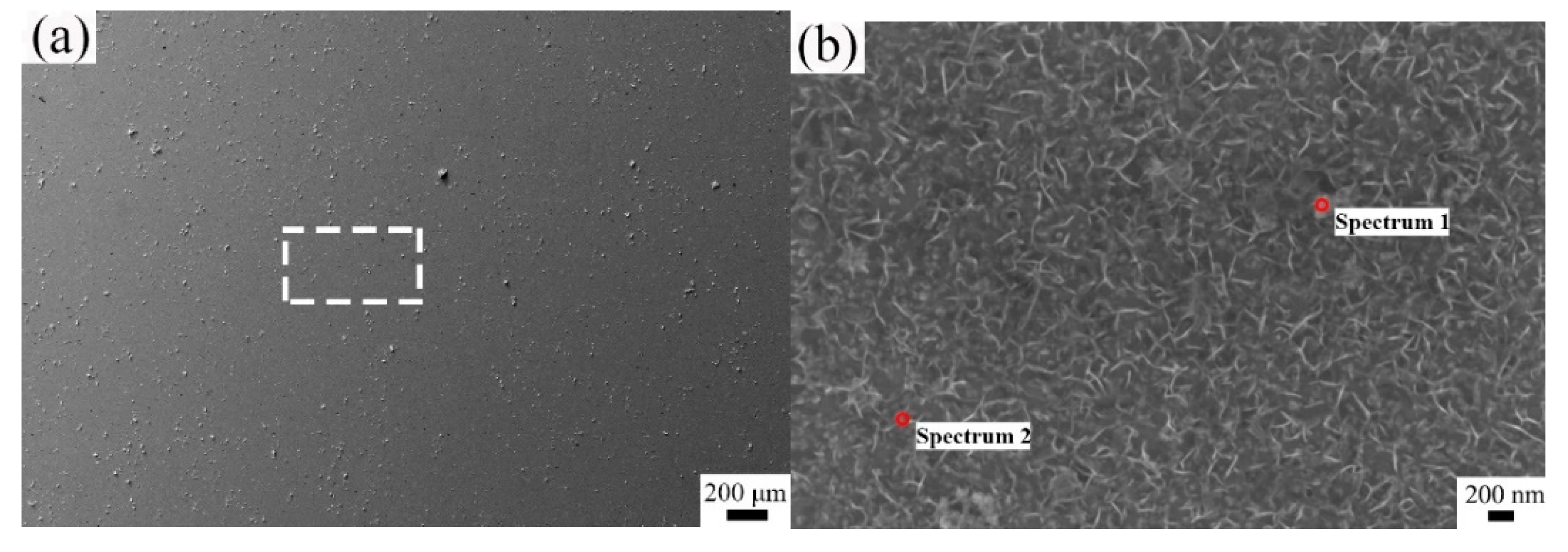
Figure 4a shows the SEM image of the corrosion scale of L245N standard steel, and Figure 4b is the enlarged image of the selected area marked in Figure 4a after 1/2 day of testing. No obvious corrosion groove can be found on the surface. There are some granular and flocculent corrosion products formed.

Table 3. EDS results of corrosion scale formed on L245N standard steel after 1/2 day corrosion test, (at. %). The spectrum labels correspond to Figure 4b.

Spectrum	C	O	Si	Cu	S	Cl	Ca	Mn	Fe
1	28.20	10.13	0.47	0.93	0.07	-	0.02	0.37	59.77
2	28.43	9.01	0.49	0.97	0.07	0.05	0.06	0.36	60.55

is the EDS result of corrosion scale formed on L245N standard steel after 1/2 day of the corrosion test. The corrosion products mainly consist of the elements of Fe, C and O. The stoichiometric ratio of O in the products is much lower than that of O in the iron oxide, which means that only a very thin corrosion scale forms on the surface after the 1/2 day test.

Figure 5a shows the SEM image of a cross-section of L245N standard steel after 1/2 day of testing. No obvious corrosion scale can be found. Figure 5b shows the enlarged SEM image of area marked by the white box in Figure 5a. The region indicated with the white dotted line is the pearlite phase, and the black band in the region with the white dotted line is cementite phase. The thin scale consisted of flocculent corrosion products mainly deposited on the surface of pearlite in the metal, however, the corrosion products on the surface of ferrite in the matrix are barely present, which indicates that corrosion products are more easily produced on pearlite under flow solution. Figure 5c is the EDS mapping of the area in the red box shown in Figure 5a. A very thin corrosion layer enriched in O can be found, and Cl cannot be found in the corrosion scale. Figure 5d shows the EDS compositional profile along red line marked in Figure 5b. The corrosion scale consists of the elements of Fe, C and O. The thickness of the thin corrosion scale is about 0.75 μm. From the above results, a very thin corrosion scale with the thickness of 0.75 μm consists of granular and flocculent corrosion products. No obvious corrosion occurs between ferrite and pearlite, which indicates the uniform corrosion of the metal occurs after 1/2 day of testing.

Figure 6a shows the SEM image of the corrosion scale of L245N standard steel after 2 days of testing. Several obvious slender and shallow band-shaped grooves can be found. Figure 6b is the enlarged image of the selected area marked in Figure 6a. Some embossed patterns in band-shaped grooves can be seen. The protrusions on the surface are remaining lamellar cementite in pearlite phase.

Table 4. EDS results of corrosion scale formed on L245N standard steel after 2 days of testing, (at. %). The spectrum labels correspond to Figure 6b.

Spectrum	C	O	Na	Cu	S	P	Ca	Mn	Fe	Ba
1	27.00	37.89	0.34	0.15	3.16	0.30	0.13	0.34	37.51	3.20
2	25.47	38.15	0.19	0.15	2.44	0.07	0.10	0.44	30.35	2.64

is the EDS result of corrosion scale formed on L245N standard steel after 2 days of corrosion testing. The corrosion products on the surface mainly contain the elements Fe, C and O, where the contents are much higher than they were after 1/2 day of testing.

Figure 7a shows the SEM image of a cross-section of L245N standard steel after 2 days of testing. It can be seen that the corrosion scale with the thickness of 0.55~5.45 μm forms. Further, the preferential dissolution can be found at the position of thick scale. Figure 7b is the enlarged SEM image of the area in the white box marked in Figure 7a. The corrosion scale consists of two layers. The inner film mainly consists of remaining laminar cementite. Its orientation is consistent with that in pearlite in matrix. The amount of remaining cementite in the corrosion scale was obtained by using the Image-Pro Plus software (Version 6.0, Media Cybernetics, Silver Spring, MD, USA ), and the value is 2.6 ± 0.3 μm² per unit length (μm) of corrosion scale. The outer film does not contain the laminar cementite. The preferential dissolution occurs for the ferrite within the pearlite. Figure 7c is the EDS mapping of the area in the red box marked in Figure 7a. A thick corrosion layer enriched in O can be found, and Cl in the corrosion scale is poor. Figure 7d shows the EDS compositional profile along the red line marked in Figure 7b. The corrosion scale consists of the elements of Fe, C and O. Its outer and inner film possess the thickness of 2 and 2.5 μm, respectively. The inner layer contains more content of Fe than that in outer layer due to the presence of the remaining cementite.

Figure 8a shows the SEM image of the corrosion scale of L245N standard steel after 4 days of testing. The band-shaped grooves similar to the previous surface can be found. Figure 8b is the enlarged image of the selected area marked in Figure 8a. The remaining cementite structure mixed with corrosion products forms a honeycomb-like surface morphology.

Table 5. EDS results of the corrosion scale formed on L245N standard steel after 4 days of testing, (at. %). The spectrum labels correspond to Figure 8b.

Spectrum	C	O	Na	P	Cu	S	Cl	Ca	Mn	Fe
1	38.29	17.08	4.94	0.20	0.08	0.14	2.37	0.26	0.44	36.20
2	35.15	26.54	6.19	0.15	0.25	0.26	2.61	0.41	0.42	30.02

is the EDS result of corrosion scale formed on L245N standard steel after 4 days of testing. The corrosion products mainly contain the elements of Fe, C and O, where the contents of O are less than that after 2 days of testing, which indicates that corrosion products are difficult to deposit on the honeycomb surfaces under flow solution.

Figure 9a shows the SEM image of a cross-section of L245N standard steel after 4 days of testing. Figure 9b is the enlarged SEM image of the area marked by the white box in Figure 9a. The thicker corrosion scale with a thickness of 6~24 μm was formed. The boundary between the scale and the metal is uneven. Obviously, the local corrosion occurs at the position of the thick scale and consisted of large amounts of remaining cementite. Figure 9c is the enlarged SEM image of the black box marked in Figure 9b. More remaining cementite structures with a thickness of 8.3~12.5 μm can be found in the corrosion scale. Compared with the original thickness of banded pearlite in metal shown in Figure 2, it can be inferred that nearly a layer of banded pearlite was corroded. The amount of remaining cementite in the corrosion scale was 3.6 ± 0.4 μm² per unit length (μm) of corrosion scale. Figure 9d is the EDS mapping of the area indicated by the red box marked in Figure 9b. The corrosion products consist of the elements of Fe, C, O and Ca. In contrast to the previous surface, Ca appears and distributes in the entire corrosion scale. A small amount of Cl can be found in the corrosion scale. Figure 9e is the EDS compositional profile along the red line marked in Figure 9b. The corrosion scale with the thickness of 24 μm is not clearly delaminated. Compared to the low content of Ca on the surface shown in Table 4, more Ca within the scale can be detected, which indicates that the corrosion products of Ca are mainly nucleus and growth in the pores of the remaining cementite under flow solution.

Figure 10a shows the SEM image of the corrosion scale of L245N standard steel after 7 days of testing. Obviously, large amounts of corrosion products deposit on the surface. Figure 10b is the enlarged image of the selected area marked in Figure 10a. The clay-like corrosion scale consists of particles with the size of 2.3~17.1 μm, and obvious holes and cracks can be found.

Table 6. EDS results of the corrosion scale formed on L245N standard steel after 7 days of testing, (at. %). The spectrum labels correspond to Figure 10b.

Spectrum	C	O	Na	Cu	S	Cl	Ca	Mn	Fe	Ba
1	15.00	63.89	2.10	0.02	-	0.42	9.01	0.09	9.11	0.36
2	18.75	61.02	0.41	-	0.01	0.04	9.56	0.10	9.74	0.38

is the EDS result of the corrosion scale formed on L245N standard steel after 7 days of testing. The corrosion products mainly contain the elementals of Fe, C, Ca and O. Compared with the results after 4 days of testing shown in Table 5, the content of Fe decreases significantly, while the content of O increases significantly, and large amounts of Ca occur. Additionally, the ratio of Fe:Ca:C:O in the corrosion scale is approximately 1:1:2:4, indicating that the corrosion scale is mainly (Fe, Ca) CO₃ deposition.

Figure 11a shows SEM image of a cross-section of L245N standard steel after 7 days of testing. Figure 11b is the enlarged SEM image of the area of the white box marked in Figure 11a. The corrosion scale with the thickness of 10~42.4 μm forms on the surface. Figure 11c is the enlarged SEM image of the area in the black box marked in Figure 11b. The white phase with lamellar structure in the corrosion scale can be considered as the remaining cementite from the dissolution of pearlite [37,38]. The corrosion scale is not clearly delaminated; nearly two layers of remaining cementite can be found in it. The amount of remaining cementite in the corrosion scale is 8.0 ± 0.3 μm² per unit length (μm) of corrosion scale. Obvious cracks and holes among the remaining cementite can be observed, indicating that the corrosion scale containing remaining cementite has a large internal stress, leading to the formation of some defects. Furthermore, some large cracks breakthrough the corrosion scale and localized corrosion under them can be observed. Meanwhile, the boundary between the matrix and the corrosion scale is uneven, and obvious remaining banded cementite structure can be seen at the boundary, indicating that localized corrosion is associated with banded pearlite. Figure 11d is the EDS mapping of the area in red box marked in Figure 11b. The corrosion scale consists of the elements of Fe, C, O and Ca; the area with remaining cementite is rich in Fe and poor in Ca. A small amount of Cl also can be found in the corrosion scale. Figure 11e is the EDS compositional profile along the red line marked in Figure 11b. Compared to the content of Ca after 4 days of corrosion testing, the higher content of Ca in the corrosion scale after 7 days of corrosion testing indicates that more corrosion products of Ca deposit, forming a thick clay-like corrosion scale.

Figure 12 shows the XRD patterns of L245N standard steel after different times. From the XRD patterns, the corrosion products after 1/2 day of testing are not detected. Only a small amount of Fe₃O₄ and remaining Fe₃C can be found after 2 days of testing; similar peaks of Fe₃C can be found in the literature [31]. Corrosion products after 4 days of testing are still Fe₃O₄ and Fe₃C, but their contents are much greater than were present after 2 days of testing, which is consistent with their SEM and EDS results. After 7 days of testing, a large number of corrosion products consisting of Fe_xCa_1−xCO₃ were found, and a small amount of Fe₃O₄ and Fe₃C can also be detected. However, phases containing Cl cannot be detected due to their low content.

Figure 13 is the image of surface morphology after removing corrosion products after different times. It can be found that the surface morphology of the sample was roughly divided into sharp and deep linear grooves, shallow and wide band grooves, pits etc. The grooves are parallel to the flow direction of rotation in the autoclave. Figure 13a,b shows the plan and stereogram images of the surface morphology after 1/2 day of testing. No obvious grooves are found, instead some micro-pits are present. Figure 13b,c shows the plan and stereogram images of the surface morphology after 2 days of testing. There are 8 linear shallow grooves, and parts of the surface show micro-pits, which indicates that some locations of L245N standard steel appears to have obvious priority corrosion. Figure 13e,f shows the plan and stereogram images of the surface morphology after 4 days of testing. There are 17 linear grooves uniformly distributed over the entire surface, showing the characteristics of uniform corrosion. They indicate that the corrosion after 4 days of testing is more extensive than that after 2 days of testing. Figure 13g,h shows the plan and stereogram images of the surface morphology after 7 days of testing—there are 20 linear grooves uniformly distributed over the entire surface. Obviously, compared to that after 4 days of testing, the number of linear grooves does not increase much, but they are deeper and wider. In addition, the Ra of surface morphology after different times was 0.335 μm, 2.769 μm, 5.414 μm and 7.945 μm, respectively. The increasing tendence of Ra with time is consistent with the change of surface morphology.

Figure 14 is the linear profile of the matrix surface of the L245N standard steel after different times. The mean and standard deviation after 1/2, 2, 4 and 7 days of testing was 13.3 ± 461.2, −56.3 ± 3366.2, −1697.9 ± 4592.4 and 237.0 nm ± 6042.4 nm, respectively. They indicate that the undulation of the matrix surface becomes more dramatic with time, which is consistent with the increasing tendence of Ra. Moreover, after 1/2 day of testing, it can be seen that 13 pits with the depth of 1.8~5.0 μm appear on the L245N standard steel, and no obvious grooves can be seen. However, obvious grooves with the average depth of 10.8 ± 5.9, 14.6 ± 4.4 and 22.4 μm ± 6.7 μm occur on the surface after 2, 4 and 7 days of testing. Additionally, the deepest groove with the depth of 33.3 μm appears after 7 days of testing. Combined with the results of Figure 13, they indicate that after 1/2 day of testing, the corrosion of L245N standard steel is slight, and only some pits occur. After 2 days of testing, some locations of the surface are preferential corroded, forming shallow grooves. After 4 days of testing, the overall surface is corroded uniformly, and the corrosion degree is slightly higher than that after 2 days of testing. After 7 days of testing, the overall surface is seriously corroded, showing the deeper and wider grooves.

The EIS results are shown in Figure 15 for L245N standard steel after different times. The Nyquist diagrams are shown in Figure 15a, the Bode diagrams are shown in Figure 15b,c. The electrical equivalent circuits (EEC) fitted by the EIS date are shown in Figure 15d,e. For the samples after 0.5, 2 and 4 days, only one semicircle can be found in Figure 15a. The diameter of the capacitive semicircle gradually increases, which indicates that the corrosion resistance of the sample increases with corrosion time [39]. To confirm the time constant, the Bode plots are added in Figure 15b,c. For the samples after 0.5, 2 and 7 days, one phase angle peak can be observed, which indicates that the EEC only contains one-time constant corresponding to the double layer. Therefore, the EEC proposed in Figure 15d can model the electrical response of the samples after 0.5, 2 and 4 days. For the sample after 7 days, a low frequency inductive loop appears beside the capacitive semicircle. Furthermore, from the Bode diagrams, the capacitive phase angle peak at the mediate frequency decreases and shifts to lower frequency. In addition, a valley can be observed at lower frequency—the phase angle at 0.01 Hz presents a small negative value. They indicate that the EEC contains two-time constants corresponding to the double layer (the first one) and the corrosion film (the second one). Therefore, the EEC proposed in Figure 15e can model the electrical response of the samples after 7 days. In Figure 15d, R_s is the resistance of the solution, Q_dl is the constant phase element (CPE) related to the double layer, R_ct is the charge transfer resistance, which is inversely proportional to the corrosion rate [40,41]. In Figure 15e, Q_f is the CPE of the corrosion product film, R_f is the resistance of the corrosion film, L represents the newly added low frequency inductor related to the enhanced galvanic effect between the lamellar cementite in the corrosion scale and the pro-eutectoid ferrite [31], and R_L is inductance resistance. The impedance of CPE (Z_CPE) is described by ${\mathrm{Z}}_{\mathrm{CPE}}={\left(\mathrm{Y}\right)}^{-1}{\left(\mathrm{jw}\right)}^{-\mathrm{n}}$, where Y is the admittance (S cm⁻² sⁿ), w is the angular frequency (rad/s)/, j is the imaginary unit, ${\mathrm{j}}^2=-1$, and n is a CPE exponent ranging from −1 to 1.

The fitting results in Figure 15a–c show that the experimental results are in good agreement with the fitting obtained by the EEC.

Table 7. Electrochemical impedance parameters fitted from EIS data.

T (day)	0.5	2	4	7
Rs/Ω·cm2	13.03	7.25	3.39	10.97
Qdl/Ω·sn·cm−2	2.63 × 10−4	1.70 × 10−4	1.56 × 10−4	8.54 × 10−4
Ceff,dl/μF·cm−2	1.30 × 10−4	5.71 × 10−5	5.57 × 10−5	7.66 × 10−5
Qdl−n	0.89	0.86	0.89	0.66
Rdl/Ω·cm2	561	1485	1741	1156
Qf/Ω·sn·cm−2	-	-	-	2.26 × 10−9
Qf−n	-	-	-	0.87
Rf/Ω·cm2	-	-	-	1425
RL/Ω·cm2	-	-	-	3287
L/H·cm2	-	-	-	70.35
Chi-square	8.2 × 10−5	1.02 × 10−3	1.35 × 10−3	6.54 × 10−6

shows the electrochemical date fitted from the EEC after different times. From 0.5 day to 4 days, R_ct increases from 561 to 1741 Ω·cm², which indicates that the corrosion resistance of the sample increases with corrosion time. However, the R_ct for the sample after 7 days decreases to 1156 Ω·cm². Furthermore, the n_dl for the samples after 0.5 days to 4 days is around 0.86~0.89 (close to an ideal capacitor, n = 1), suggesting that electrolyte/corrosion film is inhomogeneous [31]. All CPE elements in the EEC shown in Figure 15d,e present non-ideal capacitors, which can be described as a branched ladder RC network [42]. In order to obtain the effective capacitance (C_eff,dl) for the double layer, Brug et al. proposed a equation considering the R_s, R_ct, n_dl and Q_dl [42,43,44,45].

$${\mathrm{C}}_{\mathrm{eff},\mathrm{dl}}={\left[{\mathrm{Q}}_{\mathrm{dl}}{\left(\frac{1}{{\mathrm{R}}_{\mathrm{S}}}+\frac{1}{{\mathrm{R}}_{\mathrm{ct}}}\right)}^{\left({\mathrm{n}}_{\mathrm{dl}}-1\right)}\right]}^{\frac{1}{{\mathrm{n}}_{\mathrm{dl}}}}$$

(2)

By Equation (2), C_eff,dl can be obtained and is shown in Table 7. The values of C_eff,dl and R_ct are used to evaluate the protective properties of the film. The higher the impedance, the lower the capacitance, resulting in the better protective effect of the film [42,44]. Based on Table 7, for the samples in the duration of 0.5 days to 4 days, C_eff,dl decreases gradually while R_ct increases. After 7 days, C_eff,dl increases while R_ct decreases. In addition, the sample after 4 days shows the lowest C_eff,dl and highest R_ct values. They indicate that the corrosion resistance exhibits a trend of increasing followed by decreasing, which is in good agreement with the results of tendency of the corrosion rate with time.

4. Discussion

It is widely accepted that the flow corrosion process is divided into three steps: electrochemical reactions at the metal, the diffusion process of ions within the corrosion film, and convective mass transfer of ions from the oxide/water interface through the boundary layer near the surface into the bulk flow [46]. In the early stages of corrosion, the diffusion of ions was not impeded by corrosion products. The corrosion process was controlled by the reaction rate of the metal, which was related to the conductivity of the solution. Xie [47] studied the corrosion behavior of A3 carbon steel in different salinity conditions. With an increase of salinity, the content of Cl⁻ in the solution increases, promoting the hydrolysis of Fe³⁺ and generation of H⁺, and accelerating the electrochemical corrosion process of the metal matrix [48]. Thus, the L245N standard steel in high brine solution after 1/2 day of testing suffered severe corrosion.

From the results of SEM and EDS, the thickness of the corrosion scale formed after 1/2, 2, 4 and 7 days of testing was about 0.75, 0.55~5.45, 6~24 and 10~42.4 μm, respectively. After 2 days of testing, the corrosion rate decreased considerably by almost 7 times, which was related to the formation of the corrosion scale. The diffusion of ions was slowed down by the obstruction of the corrosion scale, and the corrosion process was inhibited. Thus the diffusion of ions controlled by the corrosion scale was important for CO₂ corrosion. However, over time the corrosion rate showed a trend of decreasing followed by increasing slightly. The corrosion rate tendency was inconsistent with the report of Dugstad [49].The corrosion rate was continuously accelerated with increases of remaining cementite over time, as was reported by Hao [31]. Thus, the cementite had a definite influence on the corrosion process. However, other reports claimed that the corrosion rate decreased with time due to the formation and development of the corrosion layers [13,17]. Therefore, the reciprocal effect of the corrosion scale and the remaining cementite should be considered on the CO₂ corrosion.

In the procedure of CO₂ corrosion, the cementite region acted as a cathode where hydrogen evolution reaction (HER) occurred, while ferrite region behaved as an anode where ferrite dissolution occured. Meanwhile, due to the galvanic effect inside pearlite, which consisted of lamellar cementite and ferrite beyond that between pearlite and pro-eutectoid ferrite, the lamellar ferrrite dissoluted rapidly and left lamellar cementite. Within 4 days, a cementite layer with nearly an area of 3.6 ± 0.4 μm² per unit length (μm) of corrosion scale was formed, mixing with corrosion products as the corrosion scale covered the surface of the steel; the gaps between the remaining lamellar cementite and corrosion products acted as a diffusion channel of hydrogen ions and ferrous ions. Thus, the thickness of the corrosion scale acted as the determining step of electrochemical reaction, which could be proved by the change of R_ct and C_eff,dl of samples after from 0.5 day to 4 days. However, after 7 days, with the accumulating of the remaining lamellar cementite in the corrosion scale, an area which was nearly double times than that of the sample after 4 days, some defects appeared in the corrosion scale under the flow solution. As shown in Figure 11, some cracks acted as connect channels, connecting the remaining lamellar cementite and pro-eutectoid ferrite. The electrochemical reaction was promoted by the enhanced galvanic effect between the remaining cementite and ferrite in the matrix [31]. In addition, some large cracks broke through the corrosion scale, outside the corrosion medium, and ions from the matrix surface could diffuse through them, resulting in the appearance of locazied corrosion. They all could be proved by appearance of the low frequency inductor of the sample after 7 days. Therefore, the increase of the corrosion rate after 7 days could be well explained.

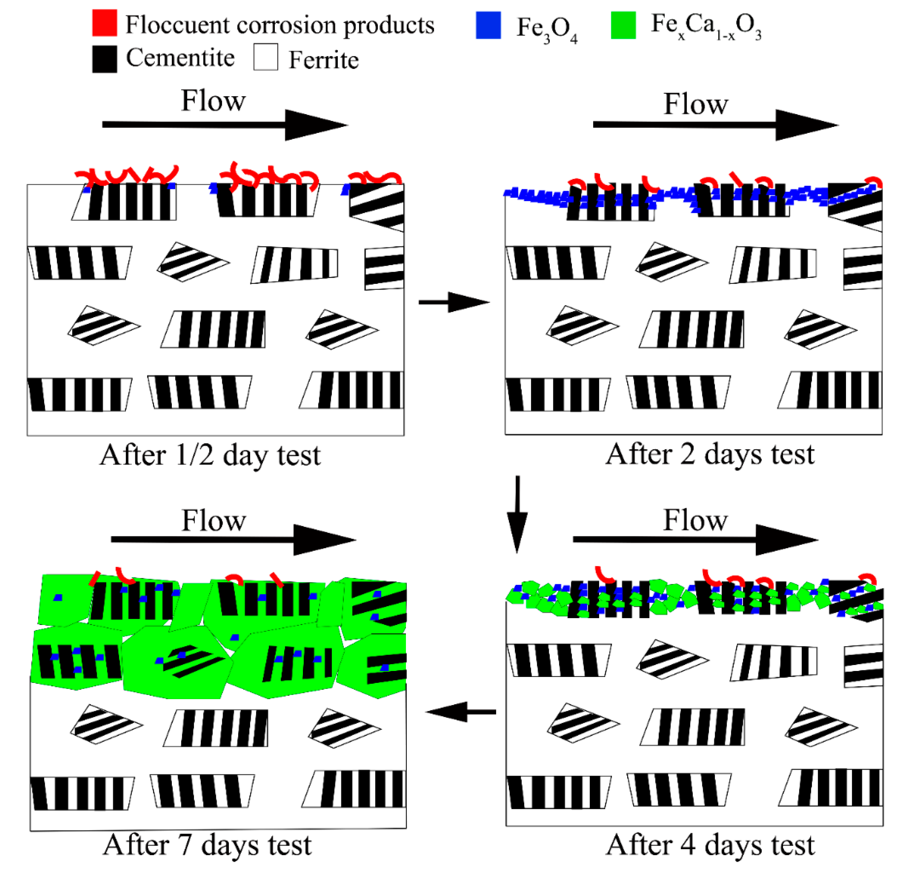
Under the effect of the flow solution, the deposition characteristics of the corrosion scale after different times were clearly different. Figure 16 shows the corrosion process with time under flow condition. Some flocculent corrosion products deposited on the surface after 1/2 day of testing, which had limited inhibition of ion diffusion. However, after 2 days of testing, some banded pearlite was corroded to leave lamellar cementite, where Fe₃O₄ deposited on their surface to form the corrosion scale. Obviously, it was more difficult for ions to pass through the cementite layer and oxide layer, resulting in the decline of the corrosion rate. After 4 days of testing, a layer of banded pearlite was corroded completely. Some corrosion products consisted of Fe_xCa_1−xCO₃ and Fe₃O₄ deposited among the remaing lamellar cementite layer, forming the thicker corrosion scale. Obviously, the thicker corrosion scale had better inhibition of ion diffusion, causing the corrosion rate to decline further. However, after 7 days of testing, the corrosion rate increased with the formation of a thick clay-like corrosion scale. The reason may be related to the formation of Fe_xCa_1−xCO₃ compound and the increasing of the remaining cementite. Calcium is bigger than iron; the density and molar volume values of Fe_xCa_1-xCO₃ formed by calcium which replaced the iron in FeCO₃ were different, forming a more porous corrosion scale, which would compromise the protective properties [17]. Thus, the continuously enhanced galvanic corrosion effect of the remaining cementite and localized corrosion caused by the poor protective Fe_xCa_1−xCO₃ scale led to the corrosion rate increase. Meanwhile, from the results of SEM, the difference in the amount of the remaining cementite formed after 2 and 4 days of testing was not significant, they were 2.6 ± 0.3 and 3.6 ± 0.4 μm² per unit length (μm) of the corrosion scale. Thus, the thicker scale played a greater effect on the corrosion process to cause the decline of the corrosion rate after 4 days of testing. In addition, there was a correlation between the deposition of Fe_xCa_1−xCO₃ and the thickness of the remaining cementite. Until a double-layer cementite skeleton formed, a significant amount of Fe_xCa_1−xCO₃ deposited and stacked, thus there was a critical thickness of the remaining cementite to produced corrosion products.

Under the effect of the mechanism of calcium ions and the remaining cementite, the surface morphology of L245N standard steel after different corrosion times can be well explained. After a short time, some areas with lower corrosion potential were inevitably corroded preferentially due to the non-uniform miscrostrucre of metal [19], forming a small number of pits. With the corrosion process, the ferrite within pearlite was preferential dissolved under high salinity flow solutions, forming a few linear grooves. Meanwhile, some remaining cementite was left, and a small amount of corrosion products were produced on the surface of the cementite skeleton. They provided a degree of protection against corrosion of the matrix. At the same time, the areas uncovered by the previous corrosion scale were corroded and overall uniform corrosion occurred, showing more linear grooves uniformly distributed over the entire surface. As more remaining cementite formed, the corrosion was aggravated by the enhanced galvanic effect between the remaining cementite and the ferrite in metal. Thus, the outside corrosion medium penetrated into the surface of the matrix and ions diffused toward the outside through the cracks and holes of the Ca_xFe_1−xCO₃ scale. Under the effect of accelerated mass transfer by flow solution, the overall surface was seriously corroded, showing the deeper and wider grooves.

5. Conclusions

• The L245N standard steel after different corrosion times had severe corrosion risk in high salinity solution due to the high conductivity of solution. Once the corrosion scale formed, the corrosion process was inhibited significantly by inhibiting ions diffusion.
• The corrosion rate decreased sharply due to the formation of the corrosion scale, but increased slightly with corrosion time, which was strongly associated with the remaining cementite by the galvanic corrosion between the remaining cementite and the ferrite within the metal. There was a critical thickness of the remaining cementite to produce the corrosion products. It was not until a double-layer cementite skeleton formed that significant amounts of Fe_xCa_1−xCO₃ deposited and accumulated.
• The uniformly formed Fe_xCa_1−xCO₃ scale with pores and cracks on the surface of the L245N standard steel was not sufficiently protective. The diffusion of ions was not inhibited, the metal was corroded deeper and wider with increasing time.

References

1. Xu, Y.; Yang, Q.; Li, Q. The Oil Well Casing’s Anti-Corrosion and Control Technology of Changqing Oilfield. Presented at the International Oil & Gas Conference and Exhibition, Beijing, China, 5–7 December 2006. Paper Number 104445. [Google Scholar]
2. Qu, C.T.; Wang, X.; Su, H.G. Corrosion factors analysis and anti-corrosion measures research of Changqing Oil Field concentrated treatment station. In Applied Mechanics and Materials; Trans Tech Publications Ltd.: Cham, Switzerland, 2013; Volume 295, pp. 1144–1148. [Google Scholar]
3. Kermani, M.; Harrop, D. The impact of corrosion on oil and gas industry. SPE Prod. Facil. 1996, 11, 186–190. [Google Scholar] [CrossRef] [Green Version]
4. Mansoori, H.; Mirzaee, R.; Esmaeilzadeh, F. Pitting corrosion failure analysis of a wet gas pipeline. Eng. Failure Anal. 2017, 82, 16–25. [Google Scholar] [CrossRef]
5. Yang, R.; Zhang, J.; Chen, H. The injectivity variation prediction model for water flooding oilfields sustainable development. Energy 2019, 189, 116317. [Google Scholar] [CrossRef]
6. Shen, Y.; Agrawal, A.; Suri, N.K. Control of microbial sulfide production by limiting sulfate dispersal in a water-injected oil field. J. Biotechnol. 2018, 266, 14–19. [Google Scholar] [CrossRef]
7. Mansoori, H.; Young, D.; Brown, B.; Singer, M. Influence of calcium and magnesium ions on CO2 corrosion of carbon steel in oil and gas production systems—A review. J. Nat. Gas Sci. Eng. 2018, 59, 287–296. [Google Scholar] [CrossRef]
8. Yang, G.; Ying, L.; Haichao, L. Experimental studies on the local corrosion of low alloy steels in 3.5% NaCl. Corros. Sci. 2001, 43, 397–411. [Google Scholar] [CrossRef]
9. Yevtushenko, O.; Bäßler, R.; Pfennig, A. Corrosion behaviour of Cr13 steel in CO2 saturated brine with high chloride concentration. Mater. Corros. 2012, 63, 517–521. [Google Scholar] [CrossRef]
10. Yevtushenko, O.; Bäßler, R. Electrochemical studies on pitting corrosion on Cr13 steel exposed to CO2 and artificial brine with high chloride concentration. In Materials Challenges and Testing for Supply of Energy and Resources; Springer: Berlin/Heidelberg, Germany, 2012; pp. 45–53. [Google Scholar]
11. Fang, H.; Brown, B.; Nešić, S.J.C. High salt concentration effects on CO2 corrosion and H2S corrosion. Presented at the CORROSION 2010, San Antonio, TX, USA, 14–18 March 2010; p. 10276. [Google Scholar]
12. Becerra, H.Q.; Retamoso, C.; Macdonald, D.D. The corrosion of carbon steel in oil-in-water emulsions under controlled hydrodynamic conditions. Corros. Sci. 2000, 42, 561–575. [Google Scholar] [CrossRef]
13. Mansoori, H.; Young, D.; Brown, B.; Nesic, S. Investigations on the CO2 Corrosion of Mild Steel in the Presence of Magnesium and Calcium Ions. In Proceedings of the NACE International Corrosion Conference Proceedings, Houston, TX, USA, 14–18 June 2020; NACE International: Houston, TX, USA, 2020; pp. 1–23. [Google Scholar]
14. Mansoori, H.; Brown, B.; Young, D.; Nesic, S. Effect of FexCayCO3 and CaCO3 Scales on the CO2 Corrosion of Mild Steel. Corrosion 2019, 75, 1434–1449. [Google Scholar] [CrossRef]
15. Ding, C.; Gao, K.W.; Chen, C.F. Effect of Ca2+ on CO2 corrosion properties of X65 pipeline steel. Int. J. Miner. Met. Mater. 2009, 16, 661–666. [Google Scholar]
16. Navabzadeh Esmaeely, S.; Choi, Y.S.; Young, D.; Nešić, S. Effect of calcium on the formation and protectiveness of iron carbonate layer in CO2 corrosion. Corrosion 2013, 69, 912–920. [Google Scholar] [CrossRef] [Green Version]
17. Tavares, L.M.; da Costa, E.M.; de Oliveira Andrade, J.J.; Hubler, R.; Huet, B. Effect of calcium carbonate on low carbon steel corrosion behavior in saline CO2 high pressure environments. Appl. Surf. Sci. 2015, 359, 143–152. [Google Scholar] [CrossRef]
18. Asahi, H.; Kushida, T.; Kimura, M. Role of microstructures on stress corrosion cracking of pipeline steels in carbonate-bicarbonate solution. Corrosion 1999, 55, 644–652. [Google Scholar] [CrossRef]
19. Clover, D.; Kinsella, B.; Pejcic, B. The influence of microstructure on the corrosion rate of various carbon steels. J. Appl. Electrochem. 2005, 35, 139–149. [Google Scholar] [CrossRef]
20. Dugstad, A.; Hemmer, H.; Seiersten, M. Effect of steel microstructure on corrosion rate and protective iron carbonate film formation. Corrosion 2001, 57, 369–378. [Google Scholar] [CrossRef]
21. Paolinelli, L.D.; Pérez, T.; Simison, S.N. The effect of pre-corrosion and steel microstructure on inhibitor performance in CO2 corrosion. Corros. Sci. 2008, 50, 2456–2464. [Google Scholar] [CrossRef]
22. Lopez, D.; Perez, T.; Simison, S.N. The influence of microstructure and chemical composition of carbon and low alloy steels in CO2 corrosion. A state-of-the-art appraisal. Mater. Des. 2003, 24, 561–575. [Google Scholar] [CrossRef]
23. Lopez, D.A.; Simison, S.; De Sanchez, S.R. The influence of steel microstructure on CO2 corrosion. EIS studies on the inhibition efficiency of benzimidazole. Electrochim. Acta 2003, 48, 845–854. [Google Scholar] [CrossRef]
24. Mishra, B.; Al-Hassan, S.; Olson, D. Development of a predictive model for activation-controlled corrosion of steel in solutions containing carbon dioxide. Corrosion 1997, 53, 852–859. [Google Scholar] [CrossRef]
25. Al-Hassan, S.; Mishra, B.; Olson, D. Effect of microstructure on corrosion of steels in aqueous solutions containing carbon dioxide. Corrosion 1998, 54, 480–491. [Google Scholar] [CrossRef]
26. Chu, R.; Chen, W.; Wang, S.H. Microstructure Dependence of Stress Corrosion Cracking Initiation in X-65 Pipeline Steel Exposed to a Near-Neutral pH Soil Environment. Corrosion 2004, 60, 275–283. [Google Scholar] [CrossRef]
27. Franceschi, M.; Pezzato, L.; Settimi, A.G.; Gennari, C.; Pigato, M.; Polyakova, M.; Konstantinov, D.; Brunelli, K.; Dabalà, M. Effect of Different Austempering Heat Treatments on Corrosion Properties of High Silicon Steel. Materials 2021, 14, 288. [Google Scholar] [CrossRef]
28. Bignozzi, M.C.; Calcinelli, L.; Carati, M.; Ceschini, L.; Chiavari, C.; Masi, G.; Morri, A. Effect of Heat Treatment Conditionson Retained Austenite and Corrosion Resistance of the X190CrVMo20-4-1 Stainless Steel. Met. Mater. Int. 2019, 26, 1318–1328. [Google Scholar] [CrossRef]
29. Hill, H.; Raab, U.; Weber, S.; Theisen, W.; Wollmann, M.; Wagner, L. Influence of heat treatment on the performance characteristics of a plastic mold steel. Steel Res. Int. 2011, 82, 1290–1296. [Google Scholar] [CrossRef]
30. Candelária, A.F.; Pinedo, C.E. Influence of the heat treatment on the corrosion resistance of the martensitic stainless steel type AISI 420. J. Mater. Sci. Lett. 2003, 22, 1151–1153. [Google Scholar] [CrossRef]
31. Hao, X.; Dong, J.; Etim, I.I.N.; Wei, J.; Ke, W. Sustained effect of remaining cementite on the corrosion behavior of ferrite-pearlite steel under the simulated bottom plate environment of cargo oil tank. Corros. Sci. 2016, 110, 296–304. [Google Scholar] [CrossRef]
32. Mora-Mendoza, J.L.; Turgoose, S. Fe3C influence on the corrosion rate of mild steel in aqueous CO2 systems under turbulent flow conditions. Corros. Sci. 2002, 44, 1223–1246. [Google Scholar] [CrossRef]
33. Videm, K.; Kvarekval, J.; Perez, T.E.; Fitzsimons, G. Surface effects on the electrochemistry of iron and carbon steel electrodes in aqueous CO2 solutions. Presented at the CORROSION 96, Denver, CO, USA, 14–19 March 1996. Paper Number: NACE-96001. [Google Scholar]
34. Nesic, S.; Lunde, L. Carbon dioxide corrosion of carbon steel in two-phase flow. Corrosion 1994, 50, 717–727. [Google Scholar] [CrossRef]
35. GB/T 9711-2011 [S]; Standardization Administration of the People’s Republic of China: Beijing, China, 2011.
36. NACE RP-0775, Preparation, Installation, Analysis and Interpretation of Corrosion Coupons in Oilfield Operations; NACE International: Houston, TX, USA, 2005.
37. Ochoa, N.; Vega, C.; Pébère, N.; Lacaze, J.; Brito, J.L. CO2 corrosion resistance of carbon steel in relation with microstructure changes. Mater. Chem. Phys. 2015, 156, 198–205. [Google Scholar] [CrossRef] [Green Version]
38. Lopez, D.A.; Schreiner, W.H.; De Sánchez, S.R.; Simison, S.N. The influence of carbon steel microstructure on corrosion layers: An XPS and SEM characterization. Appl. Surf. Sci. 2003, 207, 69–85. [Google Scholar] [CrossRef]
39. Zhang, C.; Huang, G.; Liu, Q. Research on local corrosion behavior of thermo-mechanically affected zone in dissimilar AA2024/7075 friction stir welds. Intermetallics 2021, 130, 107081. [Google Scholar] [CrossRef]
40. Bosch, J.; Martin, U.; Ress, J.; Klimek, K.; Bastidas, D.M. Influence of Thermomechanical Treatments on Corrosion of Carbon Steel in Synthetic Geopolymer Fly Ash Pore Solution. Appl. Sci. 2021, 11, 4054. [Google Scholar] [CrossRef]
41. Zhang, D.; Yang, L.; Tan, Z.; Xing, S.; Bai, S.; Wei, E.; Tang, X.; Jin, Y. Corrosion behavior of X65 steel at different depths of pitting defects under local flow conditions. Exp. Therm. Fluid Sci. 2021, 124, 110333. [Google Scholar] [CrossRef]
42. Bastidas, D.M. Interpretation of impedance data for porous electrodes and diffusion processes. Corrosion 2007, 63, 515–521. [Google Scholar] [CrossRef]
43. Brug, G.J.; van den Eeden, A.L.; Sluyters-Rehbach, M.; Sluyters, J.H. The analysis of electrode impedances complicated by the presence of a constant phase element. J. Electroanal. Chem. Interfacial Electrochem. 1984, 176, 275–295. [Google Scholar] [CrossRef]
44. Martin, U.; Bosch, J.; Ress, J.; Bastidas, D.M. Long-term stability and electronic properties of passive film of lean-duplex stainless steel reinforcements in chloride containing mortar. Constr. Build. Mater. 2021, 291, 123319. [Google Scholar] [CrossRef]
45. Martin, U.; Ress, J.; Bosch, J.; Bastidas, D.M. Stress corrosion cracking mechanism of AISI 316LN stainless steel rebars in chloride contaminated concrete pore solution using the slow strain rate technique. Electrochim. Acta 2020, 335, 135565. [Google Scholar] [CrossRef]
46. Pietralik, J.M.; Schefski, C.S. Flow and mass transfer in bends under flow-accelerated corrosion wall thinning conditions. J. Eng. Gas Turbines Power 2011, 133, 012902. [Google Scholar] [CrossRef]
47. Xie, Z.; Li, L.; Jiang, X. Study of the corrosion behavior of A3 carbon steel in simulated oilfield water. Appl. Chem. Ind. 2010, 39, 1293–1299. [Google Scholar]
48. Jiang, X.; Nešić, S.; Kinsella, B.; Brown, B.; Young, D. Electrochemical investigation of the role of Cl- on localized carbon dioxide corrosion behavior of mild steel. Corrosion 2013, 69, 15–24. [Google Scholar] [CrossRef]
49. Dugstad, A. The importance of FeCO3 supersaturation on the CO2 corrosion of carbon steels. In Corrosion’92; NACE International: Houston, TX, USA, 1992; p. 14. [Google Scholar]
Figure 1. Dimensions of the arc-shaped sample: (a) side view, and (b) vertical view.
Metals 11 00880 g001
Figure 2. (a) OM image and (b) SEM image of the metallographic structure of L245N standard steel.
Metals 11 00880 g002
Figure 3. Corrosion rate of L245N standard steel in simulated solution after different times.
Metals 11 00880 g003
Figure 4. (a) SEM images of the corrosion scales of L245N standard steel and (b) the enlarged image of the selected area marked in (a) after 1/2 day of testing.
Metals 11 00880 g004
Figure 5. (a) SEM image of the cross-section formed on L245N standard steel after 1/2 day of testing; (b) the enlarged SEM image of the area in the white box in (a); (c) EDS mapping of the area in the red box in (a) and (d) EDS compositional profile along the red line marked in (b).
Metals 11 00880 g005
Figure 6. (a) SEM image of the corrosion scale of L245N standard steel and (b) the enlarged image of the selected area marked in (a) after 2 days of testing.
Metals 11 00880 g006
Figure 7. (a) SEM image of cross-section of L245N standard steel after 2 days of testing; (b) the enlarged SEM image of the area in the white box marked in (a); (c) EDS mapping of the area in the red box in (a) and (d) EDS compositional profile along the red line marked in (b).
Metals 11 00880 g007
Figure 8. (a) SEM image of the corrosion scale of L245N standard steel and (b) the enlarged image of the selected area marked in (a) after 4 days of testing.
Metals 11 00880 g008
Figure 9. (a) SEM image of a cross-section of L245N standard steel after 4 days of testing; (b) the enlarged SEM image of the area in the white box in (a); (c) the more enlarged SEM image of the area in the black box marked in (b); (d) EDS mapping of the area in the red box in (b) and (e) EDS compositional profile along the red line marked in (b).
Metals 11 00880 g009
Figure 10. (a) SEM image of the corrosion scale of L245N standard steel and (b) the enlarged image of the selected area marked in (a) after 7 days of testing.
Metals 11 00880 g010
Figure 11. (a) SEM image of a cross-section of L245N standard steel after 7 days of testing; (b) the enlarged SEM image of the area in the white box in (a); (c) the more enlarged SEM image of the area in the black box marked in (b); (d) EDS mapping of the area in the red box in (b) and (e) the EDS compositional profile along the red line marked in (b).
Metals 11 00880 g011
Figure 12. XRD patterns of L245N standard steel after different times.
Metals 11 00880 g012
Figure 13. (a) The plan image and (b) stereogram image of surface morphology after 1/2 day of testing; (c) the plan image and (d) stereogram image of surface morphology after 2 days of testing; (e) the plan image and (f) stereogram image of surface morphology after 4 days of testing; (g) the plan image and (h) the stereogram image of surface morphology after 7 days of testing.
Metals 11 00880 g013
Figure 14. Linear profile of the matrix surface of L245N standard steel after different times.
Metals 11 00880 g014
Figure 15. EIS plots of L245N standard steel after different times: (a) Nyquist diagram; (b) Bode impedance vs. frequency diagram; (c) Bode phase angle vs. frequency diagram, and electrochemical equivalent circuits for EIS fitting after different times: (d) 0.5–4 days; and (e) 7 days.
Metals 11 00880 g015
Figure 16. The corrosion process with time under flow condition.
Metals 11 00880 g016