Modeling of Fluid Flow and Residence-Time Distribution in a Five-Strand Tundish

Abstract

Quantified residence-time distribution (RTD) provides a numerical characterization of mixing in the continuous casting tundish-thus allowing the engineer to better understand the metallurgical performance of the reactor. This study describes a computational fluid dynamic (CFD) modeling study for analyzing the flow pattern and the residence-time distribution in a five-strand tundish. Two passive scalar-transport equations were applied to separately calculate the E-curve and F-curve in the tundish. The numeric modeling result were compared to water-modeling results to validate the mathematical model. The volume fraction of different flow regions (plug, mixed and dead) and the intermixing time during the ladle changeover were calculated to study the effects of the flow control device (FCD) on the tundish performance. From the results of CFD calculations, it can be stated that a combination of the U-baffle with deflector holes and the turbulence inhibitor had three major effects on the flow characteristics in the tundish: (i) to reduce the extent of the dead volume; (ii) to evenly distribute the liquid streams to each strand and (iii) to shorten the intermixing time during the ladle changeover operation.

1. Introduction

The tundish-working as a buffer and distributor of liquid steel between the ladle and continuous casting molds-plays a key role in affecting the performance of casting and solidification, as well as the quality of final products, referred to as “Tundish Metallurgy”. With the continuing emphasis on the superior steel quality, a modern steelmaking tundish is designed to provide maximum opportunity for the control of molten steel flow, heat transfer, mixing and inclusion removal. Considerable research efforts have been made in academia and industry over many decades to fully exploit and enhance the metallurgical performance of the tundish [1,2,3,4].

In metallurgical engineering, the residence-time distribution (RTD) of the fluid is used as an index of the performance of the reactors. The RTD characteristics of a given tundish can be studied through the pulse injection of inert tracer at the inlet in the water model experiment and monitored by the change of tracer concentration at the outlet. The RTD analysis, e.g., the mean residence time, the plug flow volume, the dead volume and the mixed volume is used to estimate the tundish performance. The dye tracer visualizes the flow pattern, which may put the results obtained by the RTD analysis in proper perspective. These experimental studies provide useful input data to validate the developed mathematical model.

Two categories of RTD have been extensively investigated in the tundish: (i) E-curve, an instantaneous addition of tracer at inlet, which is used to describe the fluid flow and further to optimize the FCD designs such as weirs, dams, turbulence inhibitor and baffles; (ii) F-curve, a continuous addition of tracers, which is used to describe the chemical composition mixing during the ladle changeover operations.

A large number of mathematical modeling studies have been carried out to analyze the flow and the RTD in the tundish, including: (i) the study of FCD configurations; (ii) the study of external stirring (e.g., gas-stirring and electromagnetic stirring); (iii) the study of simulation model (e.g., fluid flow, turbulence, particle dispersion, isothermal/thermal, steady/transient). Several numeric simulation studies [5,6,7,8,9,10,11,12,13,14,15,16,17,18,19] of both fluid flow and RTD characteristics of the tundish have been presented in the literatures and summarized in

Table 1. Summary of mathematical modeling investigations on residence-time distribution (RTD) in the tundish.

Reference	Model 1	Code	Design				Numeric Model				Parameter Study 2
			Strand	Fluid 3	FCD 4	Gas	Fluid 5	Turb. 6	Inclu. 7	RTD 8
S. López-Ramirez (1998) [5]	N	-	2	S	B, TI	-	-	k-ε	-	E	SFR, FCD, TC
Vargas-Zamora (2004) [6]	N, P	-	1	W	TI, D	-	-	-	-	F	GFR
Zhong (2008) [7]	P	-	2	W	TI, D, W	N2	-	-	-	E	TC, FCD, GFR
Bensouici (2009) [8]	N, P	Fluent	1	W	W, D	-	-	k-ε	-	E	MS, FCD
Zheng (2011) [9]	N, P	CFX	2	S	TI, B	Ar	Eu	k-ε	La	E	TC, GFR, IS
Chen (2013) [10]	N, P	Fluent	1	S, W	W	Ar	Eu	k-ε	La	E	TC, FCD, IS
Chen (2015) [11]	N, P	Phoenics	1	W	SR, D, W, TI	-	-	k-ε	-	E	MS, TS, TP
Chang (2015) [12]	N, P	Fluent	7	S, W	TI, B	Ar	Eu	k-ε	La	E	GFR, FCD
Devi (2015) [13]	N, P	Fluent	2	S, W	D	Ar	Eu	k-ε	-	E	FCD, GFR
He (2016) [14]	N, P	Fluent	5	S, W	TI, B	-			-	E	TC, SFR
Neves (2017) [15]	N, P	CFX	2	W	SR, D, W	Air	Eu	k-ε	-	E	GFR, FCD
Wang (2017) [16]	N, P	Fluent	8	S	TI, F	-	-	k-ε	La	E	TC, FCD, IS
Aguilar–Rodriguez (2018) [17]	N	Fluent	1	S	-	Ar	VOF	k-ε	La	E	GFR, TC, FCD
Yang (2019) [18]	N	CFX	2	S	D, TI	-	-	k-ε	La	E	FCD, TC
Wang (2020) [19]	N	Fluent	2	S	W, TI, F	-	Eu	k-ε	La	E	IS, FCD, TC

¹ N—numeric model; P—physical model; ² SFR—steel flow rate; GFR—gas flow rate; TC—tundish configuration; MS—mesh size; TS—time step; ID—inlet depth; IS—inclusion size; FCD—flow control devices; ³ W—water; S—steel; ⁴ FCD—flow control devices; SR—stop rod; D—dam; W; weir; TI—Turbulence inhibitor; F—filter; B—baffles; ⁵ Eu—Eulerian; VOF—volume of fluid; ⁶ Turb—turbulence; ⁷ Inclu—inclusion; La—Lagrangian; ⁸ E—E-curve; F—F-curve.

. A diverse range of numeric modeling parameters (e.g., mesh size, steel flow rate, gas flow rate, inclusion size, installation of flow control devices, expression form of RTD) were applied to simulate flow characteristics in a wide range of tundish system. Majority of published data concerns the steel flow and RTD in one- or two-strand tundish. The liquid steel flow in a multistrand tundish is more complicated and many problems can occur in the actual casting process. A large temperature difference of liquid steel may exist between the multiple strands, which easily leads to the segregation and the nozzle clogging in the continuous casting mold. The optimization of flow characteristic in each strand and the balanced flow characteristics between multiple strands need to be considered. Therefore, it is more important to design and optimize FCD for the multistrand tundish.

This study focuses on the determination of the characteristics of RTD in a five-strand tundish through a CFD-based approach. In the following paper, the description of the CFD model and the theoretical basis of RTD analysis are given. Sensitivity studies of the mesh size have been conducted for the verification of the mathematical modeling. A 1:3 scale water model is used to measure the tracer concentration for the RTD curves. The CFD simulated results are in contrast with the measured results to validate the developed mathematical model. The analysis results of the fluid flow, the RTD E-curve and F-curve of the different designs are presented with the aim of achieving optimum control of the molten steel flow in the tundish.

2. CFD Model Description

The CFD software STAR-CCM+ v.13 from Siemens PLM is utilized to simulate the fluid flow and the tracer dispersion. The assumptions made for the mathematical model are described below:

• The model is based on a 3D standard set of the Navier–Stokes equations. The continuous phase is treated by a Eulerian framework (using averaged equations);
• The liquid flow was assumed to be isothermal and in steady state;
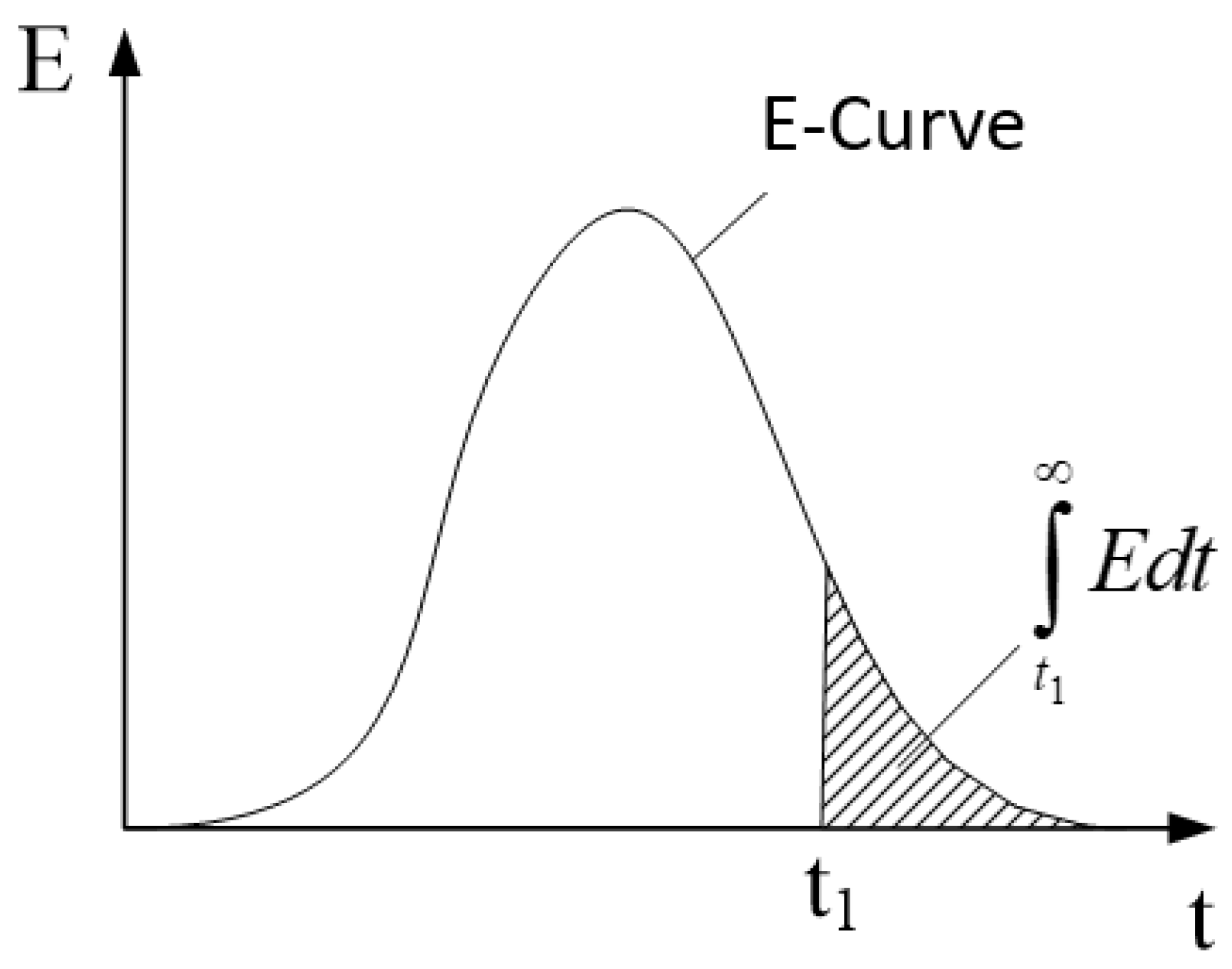
• Two additional passive scalar-transport equations are solved to separately describe the E-curve and the F-curve. Transient solver is applied to calculate the transportation of the passive scalars;
• The realizable k-ε model was used to describe the turbulence;
• The free surface is flat and kept at a fixed level. The slag layer is not included in the tundish.

2.1. Governing Equation

In the mathematical model, the conservation of a general flow variable ϕ, for example the density, momentum, within a finite control volume can be expressed as a balance between the various processes. The calculation of single-phase incompressible flow is accomplished by solving the mass and momentum conservation equations. The equations solved in CFD code are written in a general form as: [20]

$$\rho \frac{\partial \overline{\varphi }}{\partial t}+\rho \overline{u_j}\frac{\partial \overline{\varphi }}{\partial x_j}-\frac{\partial }{\partial x_j}\left[{\Gamma }_{\varphi ,eff}\frac{\partial \overline{\varphi }}{\partial x_j}\right]=S_{\varphi }$$

(1)

where ϕ represents the solved variable, Γ_ϕ,eff is the effective diffusion coefficient, S_ϕ is the source term, x_j are the Cartesian coordinates, u_j are the corresponding average velocity components, t is the time and ρ is the density. The first term expresses the rate of change of ϕ with respect to time, the second term expresses the convection (transport due to fluid-flow), the third term expresses the diffusion (transport due to the variation of ϕ from point-to-point) where Γ_ϕ is the diffusion coefficient of the entity ϕ in the phase and the fourth term expresses the source terms (associated with the creation or destruction of variable ϕ).

2.1.1. Fluid Flow

The Eulerian approach with the realizable k-ε turbulence model is applied to calculate the single-phase phenomenon in the tundish. The liquid steel flow is defined as a three-dimensional flow with the constant density. Equations (2) and (3) are the governing equations used to describe the continuous phase.

Continuity:

$$\frac{\partial \left(\rho u_j\right)}{\partial x_j}=0$$

(2)

Momentum:

$$\rho u_j\frac{\partial u_i}{\partial x_j}=-\frac{\partial P}{\partial x_i}+\frac{\partial }{\partial x_j}\left[\left(\mu +{\mu }_t\right)\left\{\frac{\partial u_i}{\partial x_j}+\frac{\partial u_j}{\partial x_i}\right\}\right]+\rho g_i+S_F$$

(3)

Realizable k-ε model: [21]

$$\frac{\partial }{\partial t}\left(\rho k\right)+\frac{\partial }{\partial x_j}\left(\rho k{u}_j\right)=\frac{\partial }{\partial x_j}\left[\left(\mu +\frac{{\mu }_t}{{\sigma }_k}\right)\frac{\partial k}{\partial x_j}\right]+G_k+G_b-\rho \epsilon -Y_M+S_k$$

(4)

$$\frac{\partial }{\partial t}\left(\rho \epsilon \right)+\frac{\partial }{\partial x_j}\left(\rho \epsilon u_j\right)=\frac{\partial }{\partial x_j}\left[\left(\mu +\frac{{\mu }_t}{{\sigma }_{\epsilon }}\right)\frac{\partial \epsilon }{\partial x_j}\right]+\rho C_{1}S\epsilon -\rho C_2\frac{{\epsilon }^2}{k+\sqrt{v\epsilon }}+C_{1\epsilon }\frac{\epsilon }{k}{C}_3{G}_b+S_{\epsilon }$$

(5)

where k is the turbulent kinetic energy; ε is the turbulent energy dissipation rate; µ is the molecular viscosity; µ_t is the turbulent viscosity; G_k represents the generation of turbulent kinetic energy due to the mean velocity; Y_M represents the contribution of the fluctuating dilatation in compressible turbulence to the overall dissipation rate; υ is the kinematic viscosity; σ_k and σ_ε are the turbulent Prandtl numbers for k and ε, respectively.

The success of numeric prediction methods depends to a great extent on the performance of the turbulence model used. The realizable k-ε model is substantially better than the standard k-ε model for many applications and can generally be relied upon to give answers that are at least as accurate. The realizable k-ε model has been implemented in STAR-CCM+ with a two-layer approach, which enables it to be used with fine meshes that resolve the viscous sublayer [22]. Though some other turbulence models (Reynolds stress model, detached eddy simulation and large eddy simulation) have been reported to be superior to others in some flow scenarios, there is no universal turbulence model that is best for all flow conditions. The total number of elements is expected to be large and turbulence models that require very fine meshes are ruled out in the first step of this study.

2.1.2. Tracer Dispersion

Tracer dispersion experiments are conducted to understand the flow pattern in the five-strand tundish. To calculate the concentration of the additive tracer, the transport of two passive scalars (E-curve and F-curve) are simulated in a Eulerian framework by solving a filtered advection–diffusion equation. The passive scalar-transport equations are solved at each time step once the fluid field is calculated.

$$\rho \frac{\partial \overline{C}}{\partial t}+\rho \overline{u_J}\frac{\partial \overline{C}}{\partial x_j}-\frac{\partial }{\partial x_j}\left[D_{eff}\frac{\partial \overline{C}}{\partial x_j}\right]=0$$

(6)

where, the effective diffusivity, D_eff, is the sum of the molecular and turbulent diffusivity. The velocity field is solved from a steady-state simulation and remained constant during the calculation of the two passive scalars [23].

2.1.3. Characteristic Volumes Calculation from RTD Curves

The RTD is a statistical representation of the time spent by an arbitrary volume of the fluid in the tundish. The RTD curve is used to analyze the different effective flow volumes, such as the plug volume, the dead volume and the mixed volume. As shown in Figure 1, E(t)dt is the probability that a fluid element enters the vessel at t = 0 and exits between time t and t + dt.

The simplest and most direct way of finding the E-curve uses a nonreactive tracer. E-curve can be plotted based on the dimensionless outlet concentration (C-curve) measured in the water model experiment. Actual mean residence time is presented in Equation (7) [24].

$$\overline{\tau }=\frac{{\int }_0^{\infty }tC\left(t\right)dt}{{\int }_0^{\infty }C\left(t\right)dt}$$

(7)

Theoretical residence time (τ) is given by:

$$\tau =V_t/Q$$

(8)

where V_t is the volume of tundish, and Q is the volumetric flow rate.

The dimensionless outlet concentration (C_i) and time (θ) are given by

$$C_i=C/C_0,\theta =\mathrm{t}/\overline{\tau }$$

(9)

$$d\theta =dt/\overline{\tau },\overline{\theta }=\overline{\tau }/\overline{\tau }=1$$

(10)

where C₀ is the concentration that corresponds to the condition where the added tracer is uniformly distributed in the tundish.

The existence of a dead volume can significantly decrease the active volume of tundish and reduce the residence times of liquid in the vessel. The increase in the dead volume fraction proves to be detrimental for the mixing.

In the tundish, the plug flow volume fraction (V_p/V_t), the mixed-flow volume fraction (V_m/V_t) and the dead-volume fraction (V_d/V_t) have been calculated through Equations (11)–(13) [25].

The dead volume fraction,

$$V_d/V_t=1-\frac{\overline{\tau }}{\tau }$$

(11)

The plug-flow volume fraction,

$$V_P/V_t=\left({\theta }_{min}+{\theta }_{peak}\right)/2$$

(12)

The mixed-flow volume fraction,

$$V_m/V_t=1-V_d/V_t-V_p/V_t$$

(13)

where, θ_min is the minimal dimensionless time at the tundish outlet and θ_peak is the peak dimensionless time at the tundish outlet.

Another common RTD expression is the cumulative distribution function F(t), i.e., the F-curve. F-curve is a fraction of the liquid that has a residence time less than time (t) and can be obtained by making a continuous addition of tracers at inlet. The concentration of tracer in the outlet stream is the F-curve. The relation between F(t) and E(t) is as follows:

$$\mathrm{F}\left(t\right)={\displaystyle \underset{0}{\overset{t}{\int }}E\left(t\right)dt}$$

(14)

Because the F-curve has the integral property, it cannot reflect the transient or local information with the same resolution as the E-curve. In this study, two passive scalar equations are solved in the CFD model: (i) an instantaneous addition of the tracer at the inlet (E-curve); (ii) a continuous addition of tracers at inlet (F-curve).

2.2. Geometry and Mesh

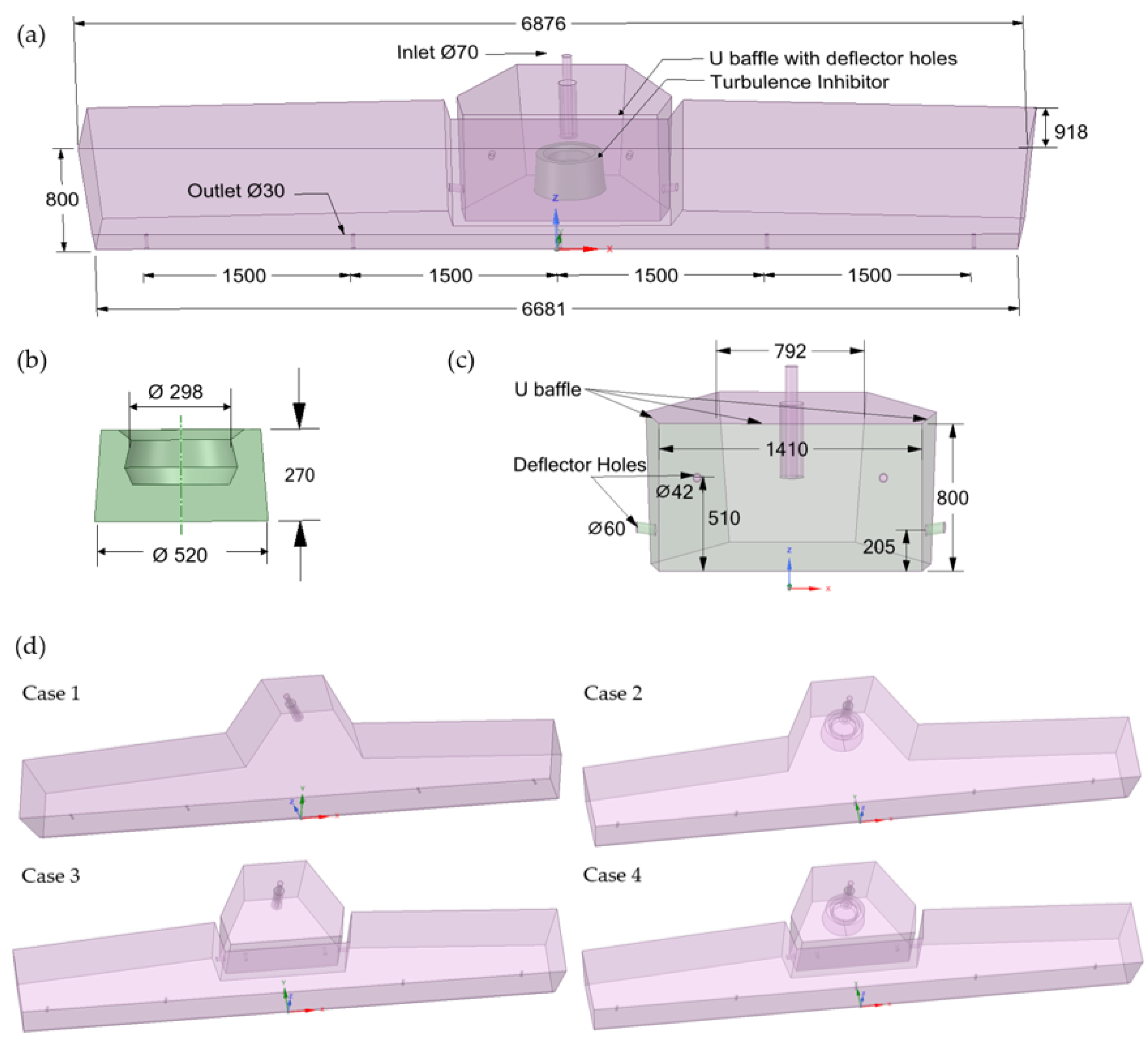
2.2.1. Tundish Geometry

The geometric dimensions of an in-plant 35-ton tundish are illustrated in Figure 2a–c. The steel flow rate is between 1.4 and 2.2 tons/min. Four cases with different tundish configurations were selected and comparatively studied (Figure 2d). They are:

• Case 1—bare tundish;
• Case 2—tundish with turbulence inhibitor (TI);
• Case 3—tundish with U-baffle with deflector holes(UB);
• Case 4—tundish with U-baffle with deflector holes and turbulence inhibitor (UB + TI).

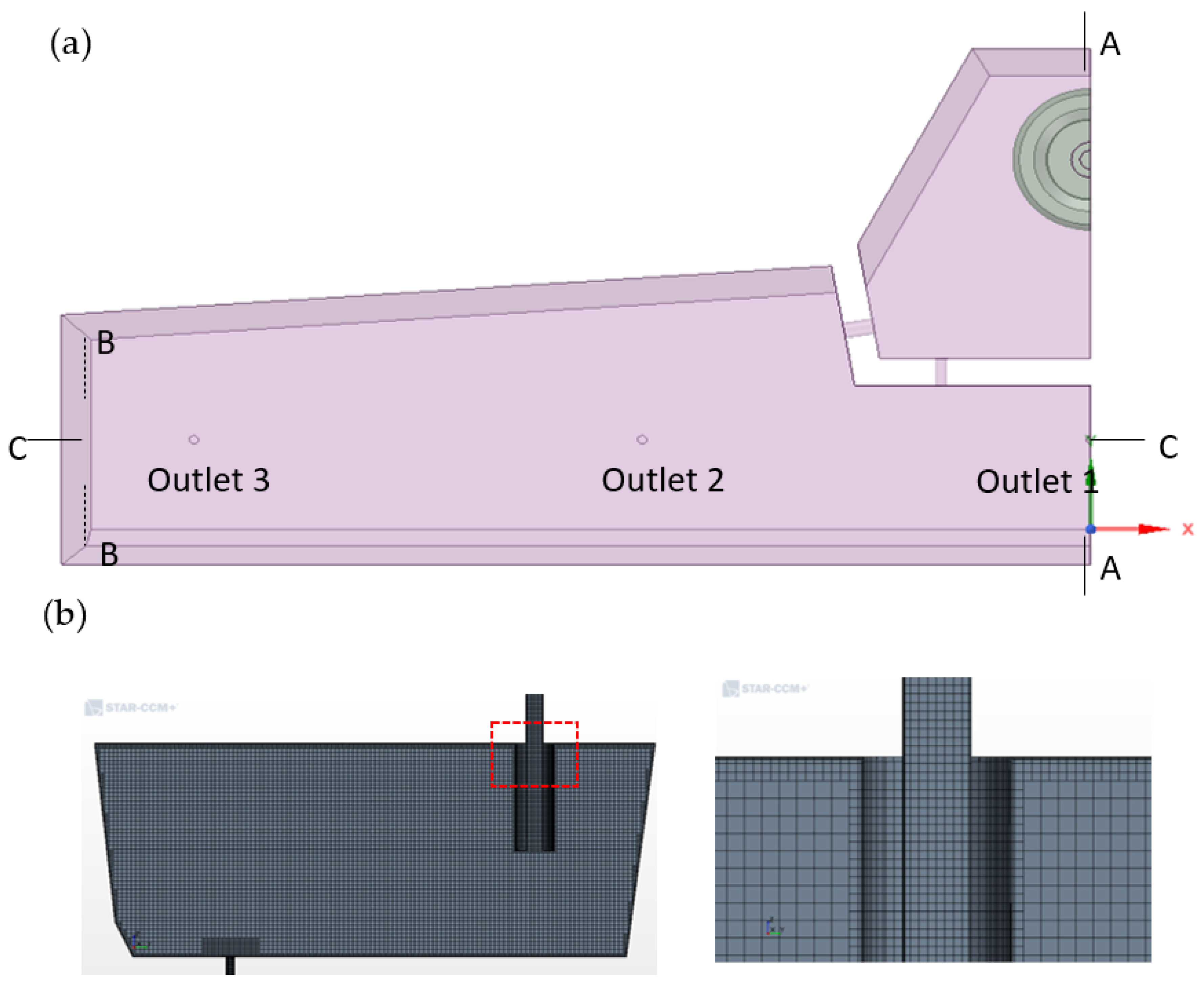
2.2.2. Computational Domain and Mesh

To create the geometry for CFD calculation, the first step was to build up a 3D-CAD model by using the Ansys Spaceclaim V19.1. Half of the water model (length scale $\frac{1}{3}$) of the five-strand tundish was taken as the computational domain considering the symmetry of the tundish, illustrated in Figure 3a. The volume mesh was generated in Star-CCM + V13.04, utilizing the trimmer and prism layer meshing options. Three prism layers were generated next to all the walls. The surface mesh was generated first. Then the volume mesh was built based on the surface mesh by adjusting the growth rate and the biggest mesh size. A base mesh size of 0.003 m was used in this study. The surface average y+ value in the first layer of the mesh near the wall was 1.5. The final CFD model had a trimmer mesh of 2 million cells in the computing domain (Figure 3b).

2.3. Initial and Boundary Conditions

2.3.1. Liquid Phase

The density and viscosity of water in numeric modeling were set to be 998 kg∙m⁻³ and 8.9 × 10⁻⁴ Pa∙s. No-slip conditions were applied at all solid surfaces for the liquid phase. Free-slip condition was applied at the free surface. A constant inlet velocity was used. At the tundish outlet, the outflow boundary condition was applied. A wall function was applied to bridge the viscous sublayer and provide the near-wall boundary conditions for the average flow and the turbulence transport equations. The wall conditions were connected by means of empirical formulae to the first grid node close to the solid surfaces.

Table 2. Parameters and boundary conditions used in simulation.

Water density	998 kg/m3
Water viscosity	0.00089 Pa·s
Reference Pressure	101,325 Pa
Inlet flow rate	0.00028 m3/s
Outlet (outflow ratio)	0.2:0.4:0.4 (Outlet 1/2/3)
Wall	No slip
Free surface	Free slip
Tracer inlet (E-curve)	1 (t <= 0–2 s), 0 (t > 2 s)
Tracer inlet (F-curve)	1

presents the parameters and boundary conditions used in the CFD simulations.

2.3.2. Tracer

Zero mass transfer flux was set at all walls and free surface for the passive scalar equation solutions. To solve the passive scalar Equation (1) for E-curve, at t = 0–2 s the mass fraction of tracer at the inlet was set to be equal to 1. When t > 2 s it was given as zero. To solve the passive scalar Equation (2) for F-curve, the mass fraction of the tracer at inlet was set to be equal to 1 for all the time steps. The concentration of the tracer at the outlet was monitored from t = 0 and the RTD curves were obtained from the numeric calculation.

2.4. Solution Procedure

The simulations were started by solving the steady state flow and the turbulence equations until a converged flow field was obtained. Then, the flow and turbulence equations were turned off. The passive scalar equations and the transient solver were activated. At this stage, the mass fraction of the tracer at the inlet boundary was defined by the user field functions.

The discretized equations were solved in a segregated manner with the semi-implicit method for the pressure-linked equations (SIMPLE) algorithm. The second-order upwind scheme was used to calculate the convective flux in the momentum equations. The solution was judged to be converged when the residuals of all flow variables were less than 10⁻⁴, together with the stability of the velocity and the turbulence at the key monitor points. The under-relaxation parameter of flow calculations for the pressure, the velocity and the turbulence were 0.2, 0.8 and 0.8, respectively.

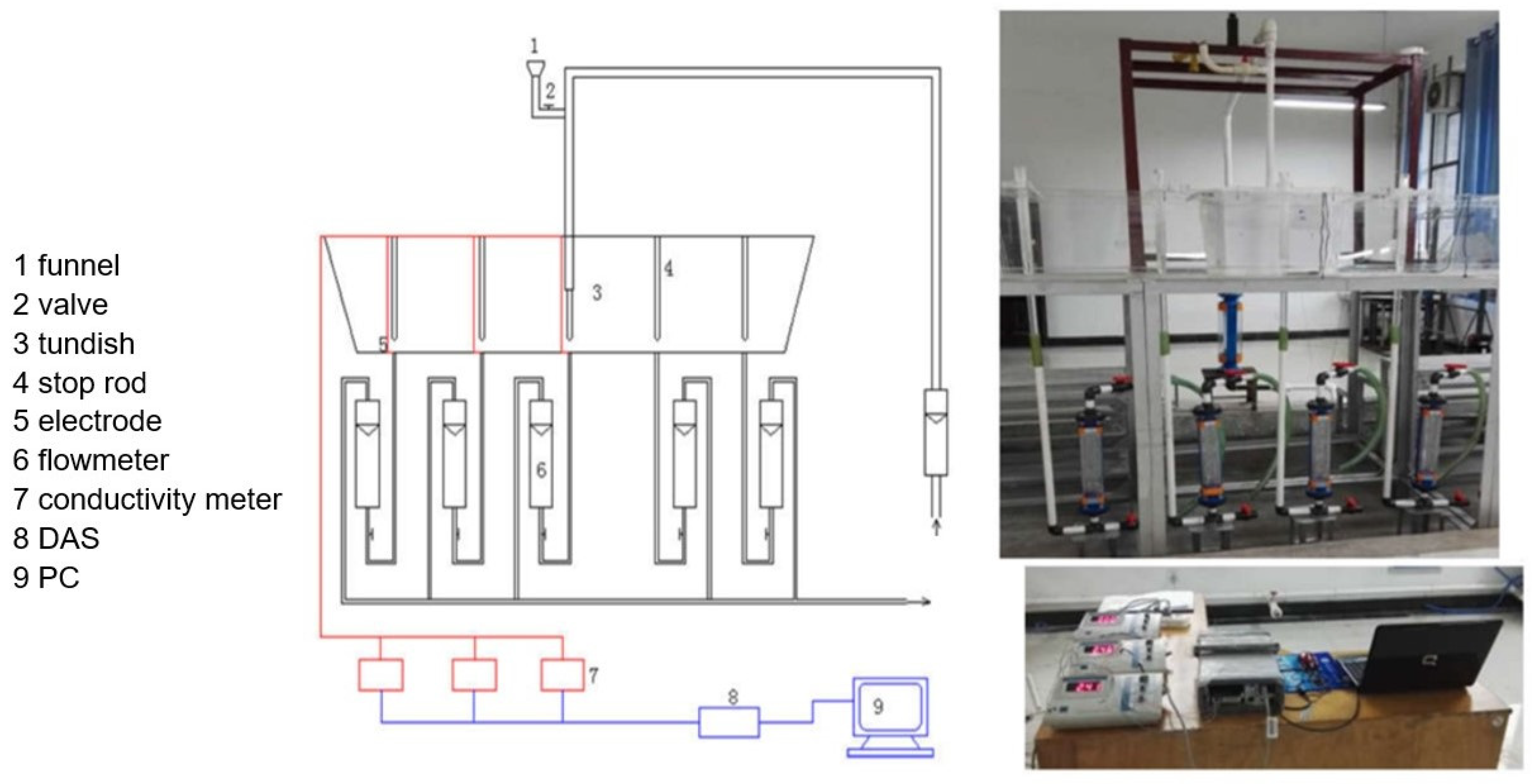
3. Water Model

The parameters used in the water model were calculated by Froude similarity criterion, according to the expression below.

Geometric similarity:

l_m/l_p = λ

(15)

Froude similarity:

Fr = u²/gl

(16)

The scaled down velocity and water flow rate are correlated according to [26]

u_m/u_p = λ^1/2

(17)

Q_m/Q_p = λ^5/2

(18)

where, Fr is the Froude number; u is the velocity(m∙s⁻¹); g is the acceleration of gravity (m∙s⁻²); l is the length (m); Q is the volumetric flow rate (m³∙s⁻¹) and λ is the length scale (1/3 in this study). The subscript m and p represent model and prototype, respectively. The volume of water model (V_m) was 0.2 m³ and the volumetric flow rate of water model (Q_m) was 0.00028 m³∙s⁻¹.

A 1:3 scale water model of the industrial prototype was used for the experimental analysis. The experimental apparatus was shown in Figure 4. The water model was made of plexiglass. The water model experiment was carried out considering the dispersion of tracer concentration in order to work out the characteristics of RTD curves. A water solution of NaCl was used as a tracer. The pulse stimulus–response technique was used to measure and obtain the RTD E-curves. When the assumed liquid level in the water model was reached and the flow was stabilized, 240 mL saturated NaCl solution was quickly poured into the inlet as a tracer within 2 s. The change of tracer concentration was registered continuously at the outlets from water model. The time and concentration were transformed to the dimensionless value in order to compare the obtained flow characteristics. Fluid flow pattern was observed by the intensity of dye tracer.

4. Results and Discussion

4.1. Validation of CFD Model

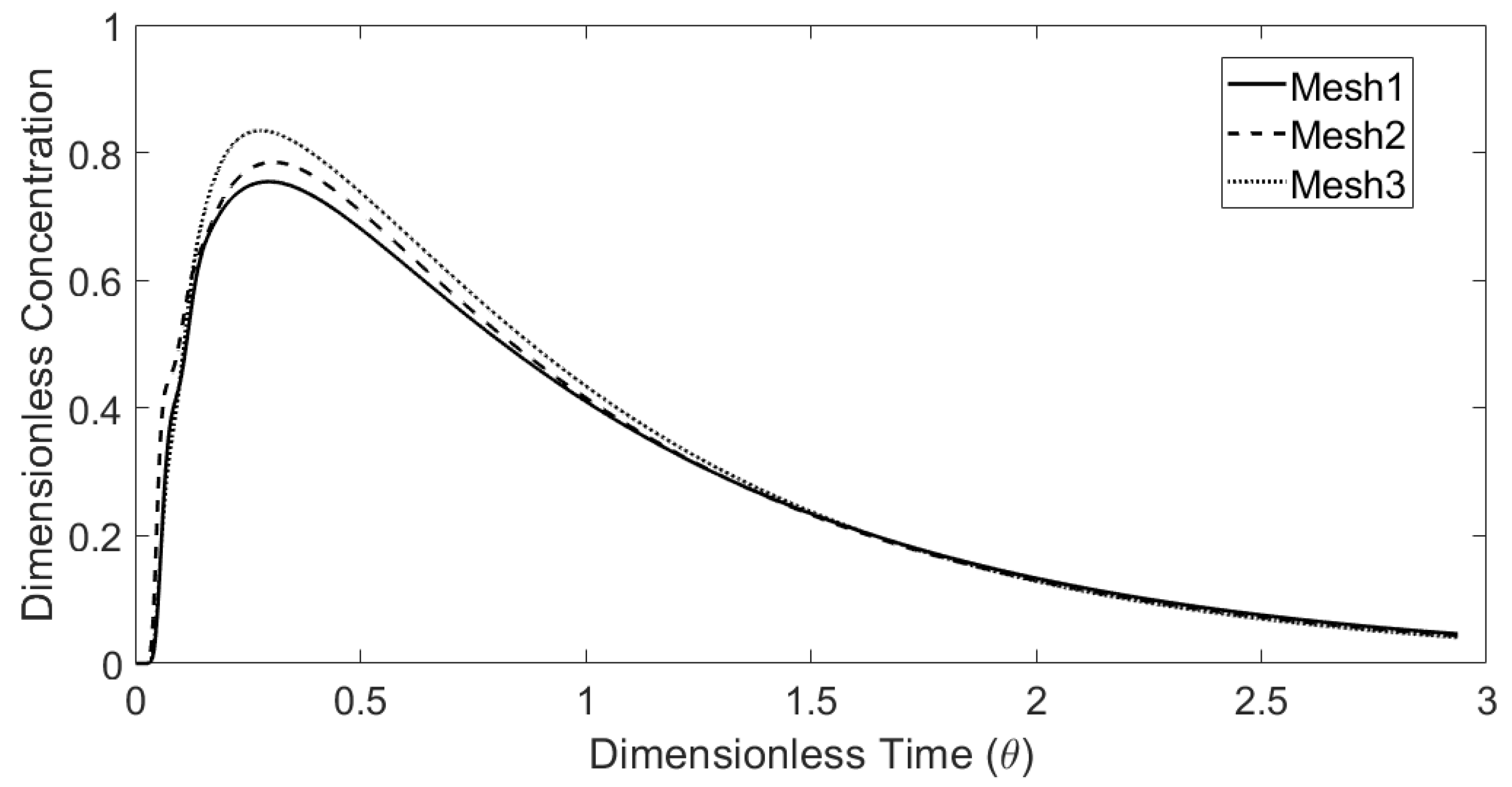
4.1.1. Independent of Computational Mesh

Utilization of an adequately refined and high-quality mesh was an important step in achieving accuracy in numeric simulations. As shown in Figure 5, a mesh independency study was carried out to estimate an appropriate mesh density for the RTD analysis.

Table 3. The computational RTD parameters and volume fraction of flow with different mesh size.

Mesh	Mesh Number	Mesh Size (m)	ttheo (s) 1	tmin (s)	tmax (s)	tmean (s)	Vp/V (%)	Vm/V (%)	Vd/V (%)
1	4 Million	0.002	749	31	222	685	17	75	9
2	2 Million	0.003	749	26	229	669	17	72	11
3	1 Million	0.004	749	30	208	664	16	73	11

¹t_theo: theoretical residence time; t_min: minimum breakthrough time; t_max: time corresponding to peak concentration; t_mean: mean residence time. V_p/V: plug flow volume fraction. V_d/V: dead volume fraction; V_m/V: mixed flow volume fraction.

displays the calculated RTD parameters and volume fraction of flow with different mesh sizes. Comparing the resulted of three mesh sizes, the difference of volume fraction of the plug flow, mixed flow and dead flow were less than 2%, 3% and 1%, respectively. An acceptable mesh independent solution was obtained based on the observations above. With the considerations of the computing load and the near wall resolution, the computations were carried out with 2 million cells (Mesh 2) and the reference mesh size was 0.003 m.

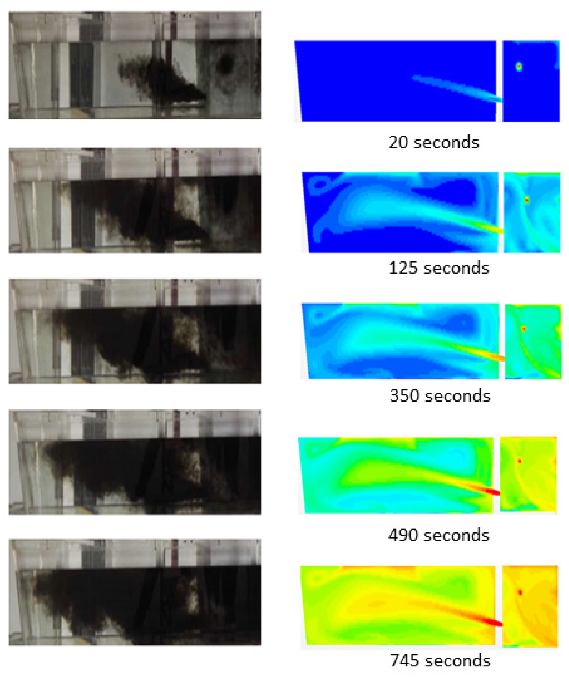
4.1.2. Numeric vs. Physical Modeling

Figure 6 shows the comparisons between the predicted and measured results of the transient tracer dispersions for Case 4—UB+TI. The tracer comes out through the deflector hole of the U-baffle, tends to flow towards to the left-side wall along the top surface. One part of the tracer flows downward towards the outlets, while another part flows straight to the left-side wall, then flows back to the outlets along the bottom of the tundish. This flow pattern extends the flow path from the inlet to the outlets, which prolongs the residence time of liquid stream and improves the mixing in the tundish. The agreement of the tracer dispersion between the numeric and physical modeling is fairly good. This demonstrates that the CFD model can be used for the simulation of the RTD in the tundish.

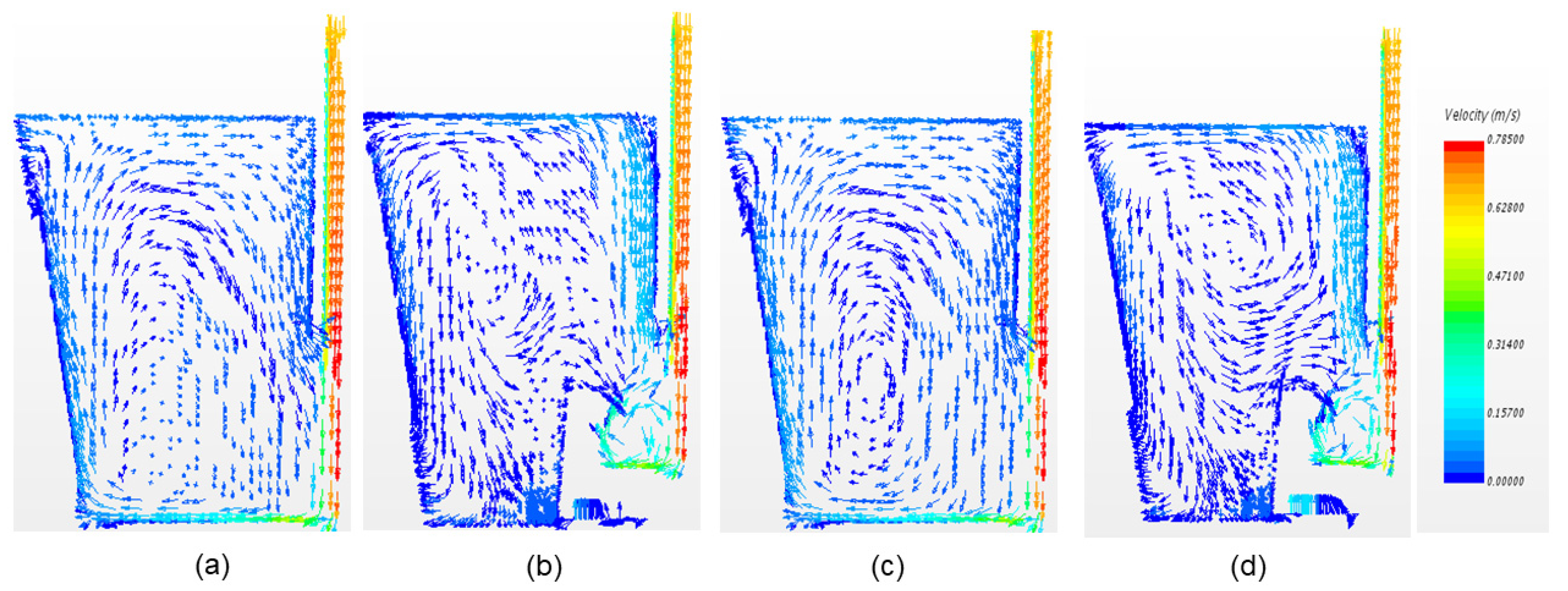
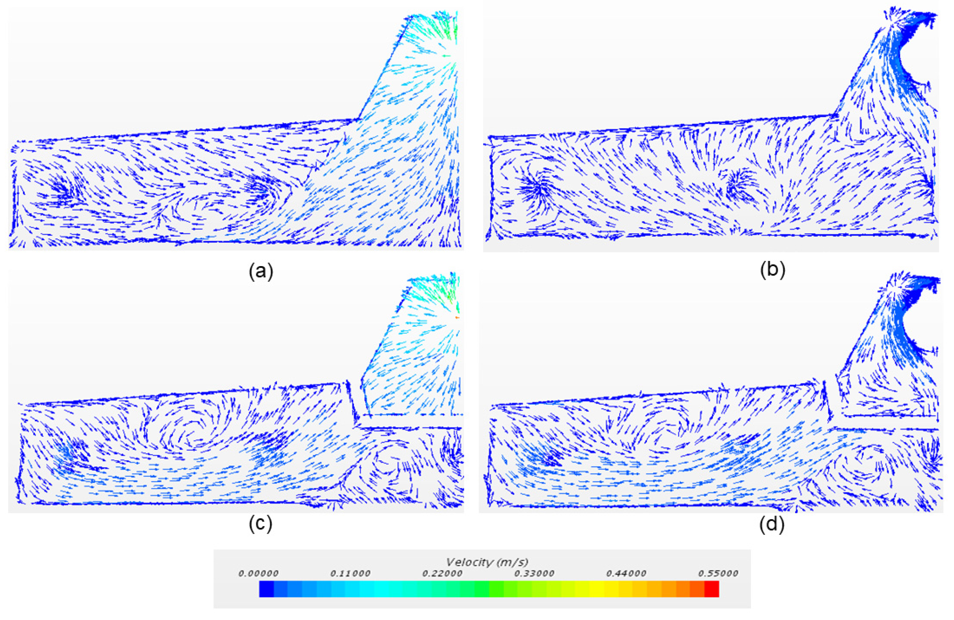
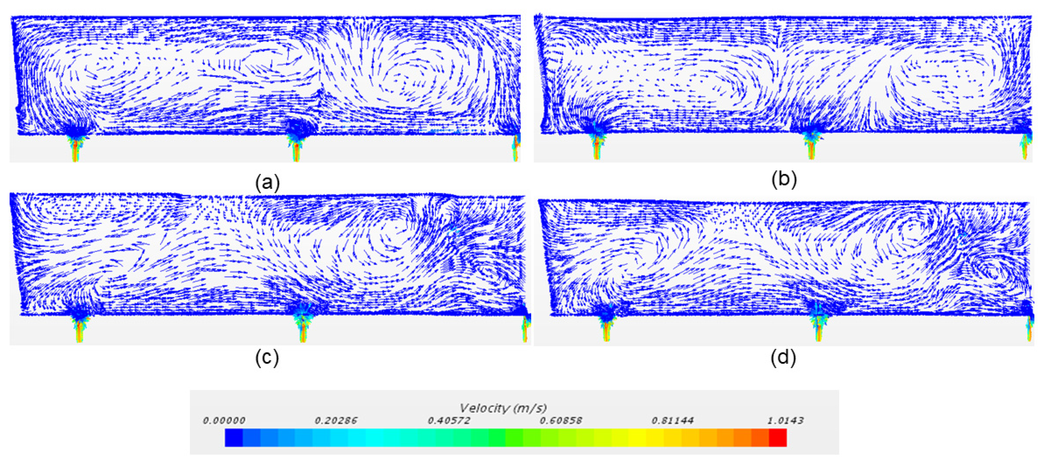
4.2. Liquid Flow in Tundish with Different FCD

The flow patterns of the four studied cases are observed and compared thorough the following view planes, as illustrated in Figure 3:

• View A: Longitudinal plane of inlet;
• View B: Horizontal plane (close to bottom);
• View C: Longitudinal plane of all the outlets.

In order to better visualize the vectors with a fine CFD mesh, some velocities were skipped by setting a geometric spacing parameter in the data postprocessing. The entering flow with high momentum hit the bottom of the tundish, moved along the sidewall of the pouring chamber and then drove back to the incoming jet, forming a clockwise recirculation nearby the inlet region (Figure 7a,c). When the tundish was equipped with turbulence inhibitor, the entering flow reoriented towards the top surface and forms a strong counterclockwise recirculation zone (Figure 7b,d). The appearance of turbulence inhibitor provided more surface directed flow with lesser turbulence on the free surface which improves the inclusions removal efficiency and also reduced the shear stress on the walls.

In Figure 8, the predicted flow patterns show that in the bare tundish, the entering flow moved along the bottom and spreads quickly into different directions in the outlet region. In the casting chamber, a high turbulence zone was observed (Figure 8a,c). The existence of turbulence inhibitor impaired the turbulence zone in the outlet chamber due to the redirection of the incoming flow (Figure 8b,d). When the flow was controlled by the U-baffle, the incoming stream could only pass through the U-baffle through the deflector holes which located in the front and side wall of the pouring chamber. The outcoming streams formed two strong recirculations near the holes (Figure 8c,d, and Figure 9c,d). The flow velocities in the center of the tundish increased due to the existence of the U-baffle (Figure 9c,d), leading to the improved mixing in the tundish.

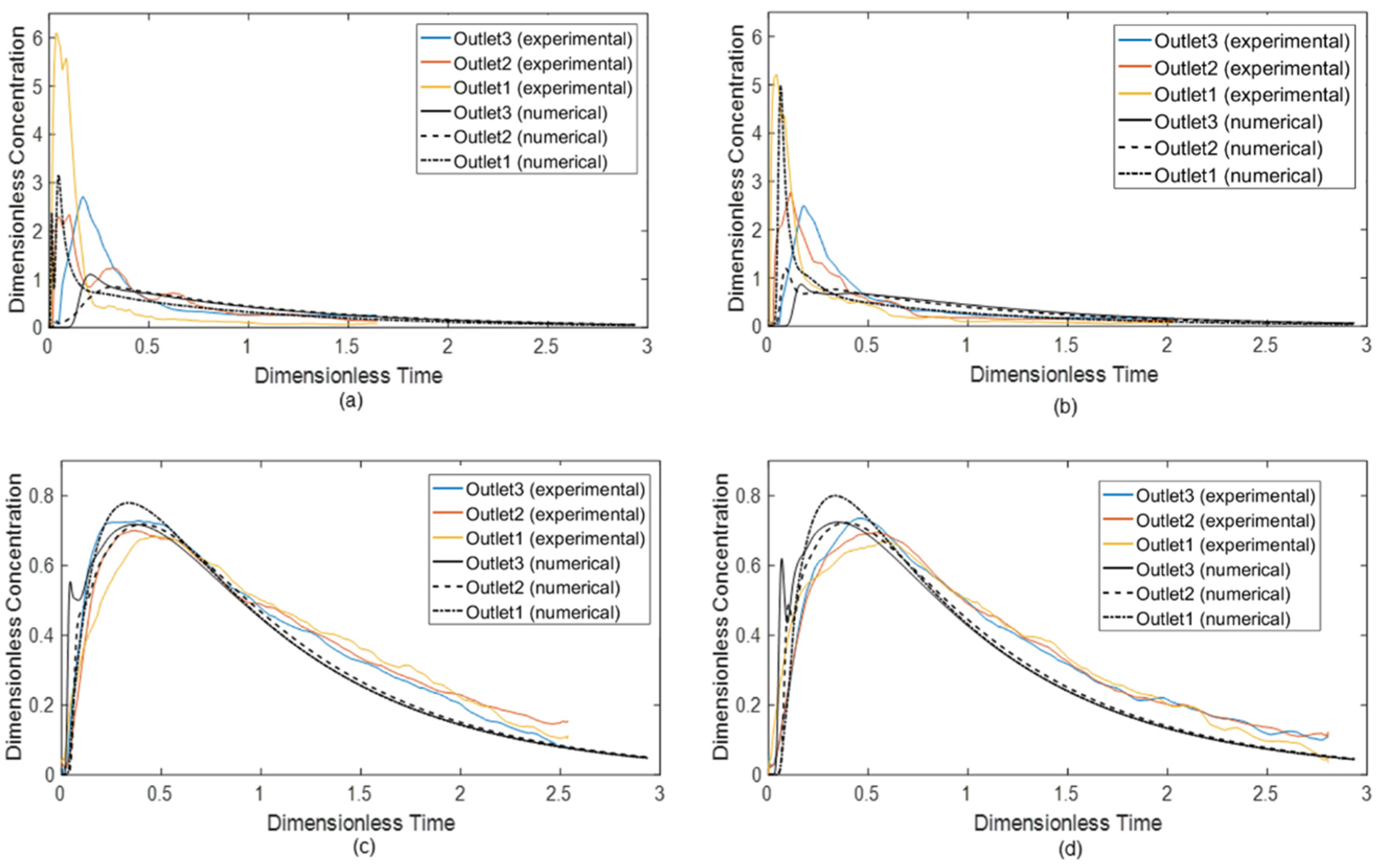
4.3. E-Curve

Figure 10 gives the E-curves through the numeric simulations and experimental measurements. As shown in Figure 10a, for the Outlet 1 in the bare tundish case, the computational breakthrough and peak concentration occurs at a relatively earlier time, 4 s and 36 s, respectively (listed in

Table 4. Computational RTD parameters and the volume fraction of flow.

Case	ttheo (s)	tmin (s)	tmax (s)	tmean (s)	Vp/V (%)	Vm/V (%)	Vd/V (%)
1—Outlet 1	749	4	36	544	3	70	27
1—Outlet 2	749	13	239	733	17	81	2
1—Outlet 3	749	78	155	711	16	79	5
2—Outlet 1	749	22	46	482	5	60	36
2—Outlet 2	749	28	65	673	6	84	10
2—Outlet 3	749	69	123	748	13	86	1
3—Outlet 1	749	27	252	696	19	74	7
3—Outlet 2	749	32	304	716	22	73	4
3—Outlet 3	749	15	274	690	19	73	8
4—Outlet 1	749	44	250	692	20	73	8
4—Outlet 2	749	44	291	707	22	72	6
4—Outlet 3	749	27	261	682	19	72	9

). A sharp rising in the tracer concentration indicates a short-circuiting flow which is undesirable in the tundish. Both the experimental and numeric E-curves present double peaks at Outlet 1, indicating that the bare tundish is associated with the considerable large dead volumes. The simulated dead volume fraction is up to 27%, which reduces the effective working space in the tundish.

The E-curves of the Case 2—TI are given in Figure 10b. The shape of the curves is similar as in Figure 10a. The predicated breakthrough time is 22 s and the dead volume fraction is 36% at Outlet 1. Furthermore, the predicted mean residence time of the three outlets is 482 s, 673 s and 748 s, respectively, showing a significant difference.

The E-curves obtained for Case 3—baffle and Case 4—baffle + turbo are analyzed in Figure 10c,d. The tundish equipped with the U-baffle could improve the flow characteristics by obtaining a more uniform liquid flow. The dead volume fractions are brought down less than 10% and the plug volume fractions are around 20% of the three outlets for both Case 3 and Case 4. The mean residence time of Outlet 1 was prolonged comparing with the cases without U-baffle. The U-baffle leads to a more uniform flow distribution in the tundish and minimizes the dead volume variance among the outlets. The optimal tundish should have a big volume fraction of the plug flow and a small volume fraction of the dead flow. When comparing Case 3 to Case 4, it shows that the turbulence inhibitor delays the breakthrough time of all the outlets but shortens the mean residence time (Table 4).

It is observed that the numeric solution differs significantly from that of the physical modeling in the initial stage, as shown in Figure 10a. The measurement uncertainties have a larger effect on the results. The possible sources of the measurement uncertainties include the mass flow rate, the amount of tracer injected, the injection rate and the conductivity measurements. A typical example is that the tracer injected through the inlet takes about several seconds and the numeric predicted breakthrough time at oulet1 is only 4 s in the bare tundish. This leads to the difficulties during the validation process. As shown in Figure 10c,d, there is a good matching of the breakthrough time between the predicted and measured results, but the measured results show a slight right shift of the RTD curves than the predicted results. The slope of E-curves after the peak is close to each other. Thus, the overall comparison between the simulation and experiment is satisfactorily close for Case 3 and Case 4. This is consistent with the observed dye trace dispersion (Figure 9).

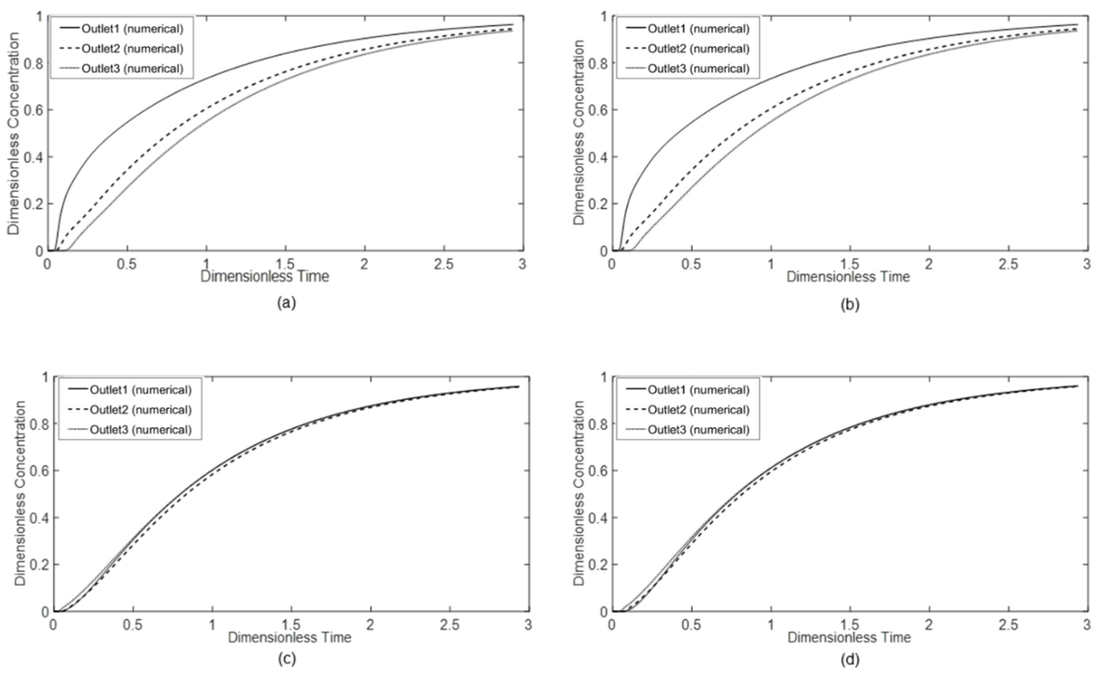
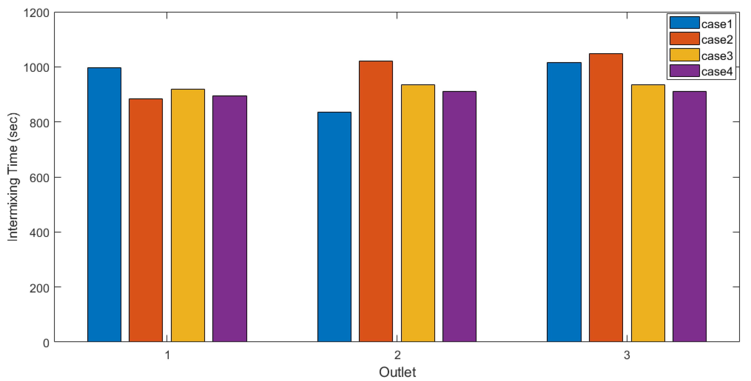
4.4. F-Curve

It was a major challenge to reduce the intermixing length of continuous casting product during the ladle changeover operation [27]. The F-curve is created by adding the tracer continuously. The F-curve results provide useful data for the prediction of the intermixing grade. Figure 11 shows the mathematical modeling results of the F-curves. The model assumes that an intermixing zone exists between the value 0.2 and 0.8 of the dimensionless concentration of the tracer.

In the Case 1—bare tundish (Figure 11a), the dimensionless concentration value of 0.2 at Outlet 1 requires relatively less time, about 82 s. This means that the new grade steel (C_tracer = 1 at the inlet) flows along a short path to the Outlet 1 as soon as it enters the tundish. The deviation for the F-curve among three outlets in Case 1 and Case 2 are bigger than that in Case 3 and Case 4. Figure 12 suggests that the predicted intermixing time related to the four studied cases. In Case 4, the tundish equipped with U-baffle and turbulence inhibitor generates the shortest intermixing time and the lowest deviation among the three outlets. This means that an optimum flow control in the tundish can shorten the intermixing zones, thereby increasing the steel yields during the mixed grade continuous casting process.

5. Conclusions

The fluid flow and the RTD curves associated with a five-strand tundish were investigated through the CFD simulations. The CFD simulated resulted were in contrast with the water model results to validate the developed mathematical model. Following conclusions can be drawn from the result:

• A combination of the U-baffle with deflector holes and turbulence inhibitor was proposed for a five-strand tundish. The existence of turbulence inhibitor impaired the turbulence zone in the outlet chamber due to the redirection of the incoming flow. Additionally, the U-type baffle with deflector holes could reorient the flow and extend the flow path, which was predicted by the numeric flow simulation and visualized through tracer dispersion in the water modeling;
• A sharp increase in the tracer concentration suggests the short-circuiting phenomena in the bare tundish, resulting in a relatively high dead volume fraction, up to 27%. High dead volume fraction was an undesirable feature in the tundish design;
• The tundish equipped with the U-baffle with deflector holes could improve the flow characteristics in the E-curve analysis. The dead volume fractions were less than 10% and the plug volume fractions were around 20% for all the outlets. The deviation around E-curves indicated a lowered difference of the flow characteristics among the outlets. The comparison of two U-baffle cases showed that the existence of turbulence inhibitor delays the breakthrough time, but shortened the mean residence time;
• Intermixing time of the mixed grade casting were numerically investigated for the ladle changeover operation by the analysis of the F-curve. A slope change of F-curve was observed when there was a short-circuiting phenomenon. The tundish equipped with U-baffle and turbulence inhibitor generated the shortest intermixing time and the lowest deviation at the outlets.

References

- Mazumdar, D.; Guthrie, R.I.L. The physical and mathematical modelling of continuous casting tundish systems. ISIJ Int. 1999, 39, 524–547. [Google Scholar] [CrossRef]
- Chattopadhyay, K.; Isac, M.; Guthrie, R.I.L. Physical and mathematical modelling of steelmaking tundish operations: A review of the last decade (1999–2009). ISIJ Int. 2010, 50, 331–348. [Google Scholar] [CrossRef] [Green Version]
- Mazumdar, D. Review, analysis, and modeling of continuous casting tundish systems. Steel Res. Int. 2019, 90, 1800279. [Google Scholar] [CrossRef]
- Szekely, J.; Ilegbusi, O. The Physical and Mathematical Modeling of Tundish Operations; Springer: New York, NY, USA, 1989. [Google Scholar]
- López-Ramírez, S.; Palafox-Ramos, J.; Morales, R.D.; Barrón-Meza, M.A.; Toledo, M.V. Effects of tundish size, tundish design and casting flow rate on fluid flow phenomena of liquid steel. Steel Res. 1998, 69, 423–428. [Google Scholar]
- Vargas-Zamora, A.; Palafox-Ramos, J.; Morales, R.D.; Díaz-Cruz, M.; Barreto-Sandoval, J.D.J. Inertial and buoyancy driven water flows under gas bubbling and thermal stratification conditions in a tundish model. Metall. Mater. Trans. B 2004, 35, 247–257. [Google Scholar] [CrossRef]
- Zhong, L.C.; Li, L.Y.; Wang, B.; Zhang, L.; Zhu, L.X.; Zhang, Q.F. Fluid flow behaviour in slab continuous casting tundish with different configurations of gas bubbling curtain. Ironmak. Steelmak. 2008, 35, 436–440. [Google Scholar] [CrossRef]
- Bensouici, M.; Bellaouar, A.; Talbi, K. Numerical investigation of the fluid flow in continuous casting tundish using analysis of RTD curves. J. Iron Steel Res. Int. 2009, 16, 22–29. [Google Scholar] [CrossRef]
- Zheng, M.J.; Gu, H.Z.; Ao, H.; Zhang, H.X.; Deng, C.J. Numerical simulation and industrial practice of inclusion removal from molten steel by gas bottom blowing in continuous casting tundish. J. Min. Metall. Sec. B Metall. 2011, 47, 137–147. [Google Scholar]
- Chen, D.F.; Xie, X.; Long, M.J.; Zhang, M.; Zhang, L.L.; Liao, Q. Hydraulics and mathematics simulation on the weir and gas curtain in tundish of ultrathick slab continuous casting. Metall. Mater. Trans. B 2013, 45, 200. [Google Scholar] [CrossRef]
- Chen, C.; Jonsson, L.T.I.; Tilliander, A.; Cheng, G.G.; Jönsson, P.G. A mathematical modeling study of tracer mixing in a continuous casting tundish. Metall. Mater. Trans. B 2015, 46, 169–190. [Google Scholar] [CrossRef]
- Chang, S.; Zhong, L.; Zou, Z. Simulation of flow and heat fields in a seven-strand tundish with gas curtain for molten steel continuous-casting. ISIJ Int. 2015, 55, 837–844. [Google Scholar] [CrossRef] [Green Version]
- Devi, S.; Singh, R.; Paul, A. Role of tundish argon diffuser in steelmaking tundish to improve inclusion flotation with CFD and water modelling studies. Int. J. Eng. Res. Technol. 2015, 4, 213–218. [Google Scholar]
- He, F.; Zhang, L.Y.; Xu, Q.Y. Optimization of flow control devices for a T-type five-strand billet caster tundish: Water modeling and numerical simulation. Chin. Foundry 2016, 13, 166–175. [Google Scholar] [CrossRef]
- Neves, L.; Tavares, R.P. Analysis of the mathematical model of the gas bubbling curtain injection on the bottom and the walls of a continuous casting tundish. Ironmak. Steelmak. 2017, 44, 559–567. [Google Scholar] [CrossRef]
- Wang, X.Y.; Zhao, D.T.; Qiu, S.T.; Zou, Z.S. Effect of tunnel filters on flow characteristics in an eight-strand tundish. ISIJ Int. 2017, 57, 1990–1999. [Google Scholar] [CrossRef] [Green Version]
- Aguilar-Rodriguez, C.E.; Ramos-Banderas, J.A.; Torres-Alonso, E.; Solorio-Diaz, G.; Hernández-Bocanegra, C.A. Flow characterization and inclusions removal in a slab tundish equipped with bottom argon gas feeding. Metallurgist 2018, 61, 1055–1066. [Google Scholar] [CrossRef]
- Yang, B.; Lei, H.; Zhao, Y.; Xing, G.; Zhang, H. Quasi-symmetric transfer behavior in an asymmetric two-strand tundish with different turbulence inhibitor. Metals 2019, 9, 855. [Google Scholar] [CrossRef] [Green Version]
- Wang, Q.; Liu, Y.; Huang, A.; Yan, W.; Gu, H.; Li, G. CFD Investigation of effect of multi-hole ceramic filter on inclusion removal in a two-strand tundish. Metall. Mater. Trans. B 2020, 51, 276–292. [Google Scholar] [CrossRef]
- Patankar, S.V. Numerical Heat Transfer and Fluid Flow; Hemisphere Publishing Corporation, Taylor & Francis Group: New York, NY, USA, 1980; ISBN 0-89116-522-3. [Google Scholar]
- Shih, T.H.; Liou, W.W.; Shabbir, A.; Yang, Z.; Zhu, J. A New k-ε eddy viscosity model for high reynolds number turbulent flows-model development and validation. Comput. Fluids 1994, 24, 227–238. [Google Scholar] [CrossRef]
- Siemens. STAR-CCM+ Version 13.04 User Guide; Siemens PLM Software: Munich, Germany, 2019. [Google Scholar]
- Ghirelli, F.; Hermansson, S.; Thunman, H.; Leckner, B. Reactor residence time analysis with CFD. Prog. Comput. Fluid Dyn. 2006, 6, 241–247. [Google Scholar] [CrossRef]
- Spalding, D.B. A note on mean residence-times in steady flows of arbitrary complexity. Chem. Eng. Sci. 1958, 9, 74–77. [Google Scholar] [CrossRef]
- Jha, P.K.; Dash, S.K. Effect of outlet positions and various turbulence models on mixing in a single and multi strand tundish. Int. J. Numer. Methods Heat Fluid Flow 2002, 12, 560–584. [Google Scholar] [CrossRef]
- Sahai, Y.; Emi, T. Criteria for water modeling of melt flow and inclusion removal in continuous casting tundishes. ISIJ Int. 1996, 36, 1166–1173. [Google Scholar] [CrossRef]
- Michalek, K.; Gryc, K.; Tkadleckova, M.; Bocek, D. Model study of tundish steel intermixing and operational verification. Arch. Metall. Mater. 2012, 57, 291–296. [Google Scholar] [CrossRef] [Green Version]