Holistic Approach on the Research of Yielding, Creep and Fatigue Crack Growth Rate of Metals Based on Simplified Model of Dislocation Group Dynamics

Abstract

The simplified model of numerical analyses of discrete dislocation motion and emission from a stressed source was applied to predict the yield stress, dislocation creep, and fatigue crack growth rate of metals dominated by dislocation motion. The results obtained by these numerical analyses enabled us to link various dynamical effects on the yield stress, dislocation creep, and fatigue crack growth rate with the experimental results of macroscopic phenomena, as well as to link them with theoretical results obtained by the concept of static, continuously distributed infinitesimal dislocations for the equilibrium state under low strain or stress rate conditions. This will be useful to holistic research approaches with concern for time and space scales, that is, in a time scale ranging from results under high strain rate condition to those under static or low strain rate condition, and in a space scale ranging from meso-scale to macro-scale mechanics. The originality of results obtained by these analyses were found by deriving the analytical formulations of number of dislocation emitted from a stressed source and a local dynamic stress intensity factor at the pile-up site of dislocations as a function of applied stress or stress rate and temperature material constants. This enabled us to develop the predictive law of yield stress, creep deformation rate, and fatigue crack growth rate of metals dominated by dislocation motion. Especially, yielding phenomena such as the stress rate and grain size dependence of yield stress and the delayed time of yielding were clarified as a holistic phenomenon composed of sequential processes of dislocation release from a solute atom, dislocation group moving, and stress concentration by pile-up at the grain boundary.

1. Introduction

The purpose of the research of dislocation mechanics is considered to have two directionalities, that is, application to the research of materials science and application to the research of the strength of materials such as that of yielding and fatigue crack growth rate.

The former closely relates to micro plasticity, such as the conditions of dislocation emission, annihilation, and cross slip, and this research was developed in the manner of the modern dislocation dynamics [1].

The latter closely relates to connect problems of the strength and fracture of materials with the macro scale [2,3,4,5].

This article is related to the fracture of materials. For this case, the numerical results of the number of moving dislocations emitted from a stressed source and local stress concentration caused by a dislocation pile-up were necessary to be formulated as an analytical function of applied stress or stress rate, temperature, and material constants [2,3].

Since the behaviors of dislocation group motion have a scale of μm at the meso-scale level, that is, the intermediate scale of nm (an individual dislocation) and mm (crack length) scales, which is a comparable scale with grain size. At this scale, the simplification of the model of analysis is considered to be more convenient to derive a predictive law of the strength and fracture of metals.

To fulfil this purpose, in our research, the establishment of a predictive theory of strength and fracture of materials was conducted by conducting the simplification of the model of analysis [3] and verification with experimental results [3,6].

Yielding phenomena such as stress rate and grain size dependence of yield stress and delayed time of yielding were especially clarified as a holistic phenomenon composed of sequential processes of dislocation release from a solute atom [7,8], dislocation group moving [6], and stress concentration by a pile-up at the grain boundary [2,3,4].

2. Dislocation Groups Dynamics Aimed for Applications to Problems of Yielding, Creep, and Fatigue [2,9,10]

2.1. Model, Basic Equation and Method of Analysis [2,9,10]

Plastic deformation is caused by dislocation group motion emitted from a stressed source.

It closely relates to plastic yielding and fatigue crack growth dominated by discrete dislocations emitted from a stressed source near a crack tip. Pioneering works on the analysis of discrete dislocation group dynamics emitted from a stressed source have been conducted [4,11,12], but a power law equation has been adopted between the isolated dislocation velocity and the stress for practical application to the strength of materials such as the yield stress, creep rate, and fatigue crack growth rate; this is given by Equation (1), which is related to experimental equations [4].

Equations of discrete moving dislocation groups are given by Equations (1) and (2).

$$V_i=\frac{d{x}_i}{dt}=M{\tau }_{eff,i}{}^m$$

(1)

$${\tau }_{eff,i}=\dot{\tau }t+A{\displaystyle \sum }_{\begin{array}{c}j=1\\ i\ne j\end{array}}^n\frac{1}{x_i-x_j}\left(i=1~n\right)$$

(2)

In the equations, V_i and $x_i$ are velocity and position of individual dislocations in a linear array, respectively, and M and m are the material constants of an isolated dislocation given by the experimental Equation (3) [13]. The calculation starts at the time of t = 0.0 s.

$$\mathrm{v}=v_0{\left(\frac{\tau }{{\tau }_0^{*}}\right)}^{m}V$$

(3)

In Equation (3), $\dot{\tau }$ is the stress rate; t is the time of stress application; ${\tau }_{eff,i}$ is the effective stress exerted on individual dislocations in terms of shear stress; and $A=\frac{Gb}{2\pi \left(1-\nu \right)}$, where G is the shear modulus, b is the Burgers vector, ν is the Poisson’s ratio, V₀ = 1 cm/s, and ${\tau }_0^{*}$ is a constant representing the stress required to give a dislocation velocity v = 1 cm/s (resistant stress against the dislocation motion).

A free expansion model of linear dislocation motion emitted from a stressed source, S, is shown in Figure 1 [9,10].

The numerical analyses were conducted as follows [9].

When the effective stress exerted on dislocation source (x = 0.0) takes the source activation stress, the new dislocation is originated at x = 0.0, and these processes are iterated. Equations (2) and (1) were solved by the Runge–Kutta Merson method. The effective stress exerted on a dislocation source is given by Equation (4).

$$\mathsf{\tau }=\dot{\tau }t$$

$${\mathsf{\tau }}_{eff,s}=\dot{\dot{\tau }t-A{\displaystyle \sum }_{j=1}^n\frac{1}{x_j}}$$

(4)

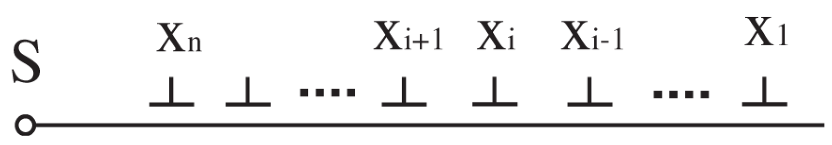
2.2. Discrete Dislocation Groups Dynamics of Free Expansion and Similarity Law of Dislocation Flow [9,10]

From the analysis, the ratio of positions, velocity and effective stress of individual dislocation in the dislocation array to those of an isolated dislocation, such as $\raisebox{1ex}{$x_i$}\!\left/ \!\raisebox{-1ex}{$x_{iso}$}\right.$, $\raisebox{1ex}{$v_i$}\!\left/ \!\raisebox{-1ex}{$v_{iso}$}\right.$, and $\raisebox{1ex}{${\tau }_{eff}{}_i$}\!\left/ \!\raisebox{-1ex}{${\tau }_{iso}$}\right.$, were found to dominated by $\mathsf{\Theta }={\left(\raisebox{1ex}{$\dot{\tau }$}\!\left/ \!\raisebox{-1ex}{${\dot{\tau }}_0$}\right.\right)}^{\raisebox{1ex}{$\left(m+1\right)$}\!\left/ \!\raisebox{-1ex}{$\left(m+2\right)$}\right.}\theta$, which is named the dynamic factor [9,10]. Here, $\tau$ is the applied stress acting on dislocations in the dislocation array, $\theta$ is the non-dimensional time controlled by $t_0$, and $t_0$ is the time of an isolated dislocation moving the distance, $l$. It is given by $t_0={\left[\frac{\left(m+1\right)l}{M{\dot{\mathsf{\tau }}}_0^m}\right]}^{\raisebox{1ex}{$1$}\!\left/ \!\raisebox{-1ex}{$\left(m+1\right)$}\right.}$ [2,9,10] by using Equation (3). In this analysis, $l$ was taken as the length of 0.01 mm.

Furthermore, the number of dislocations emitted from a stressed source were also found to be given by the dynamic factor, $\mathsf{\Theta }$, which is a non-dimensional character, as shown in Equation (5a); the dimensional parameter $\eta$ is shown in Equation (5b) [9,10].

$$\mathrm{N}=A{\mathsf{\Theta }}^{m+1}$$

(5a)

$$\mathrm{N}=A_0{\eta }^{m+1}$$

(5b)

$$\mathsf{\eta }={\dot{\tau }}^{\frac{m+1}{m+2}}t=\tau {\dot{\tau }}^{-\frac{1}{m+2}}$$

In the equation, A and A₀ are non-dimensional and dimensional constants, respectively.

By dimensional analysis, N is given by Equation (6a) [9,10].

$$\mathrm{N}=\gamma \left(\mathrm{m}\right){\left(\raisebox{1ex}{$M$}\!\left/ \!\raisebox{-1ex}{$Gb$}\right.\right)}^{\left(\frac{m+1}{m+2}\right)}{\eta }^{m+1}$$

(6a)

$$\gamma \left(\mathrm{m}\right)=1.4m^{-1.45}$$

(6b)

In these equations, $\mathsf{\gamma }\left(\mathrm{m}\right)$ is a non-dimensional function depending on m.

The velocity of an isolated dislocation is given by thermally activated process, as shown in Equation (2) [14].

$$\mathrm{v}=A_{1}exp\left(-\frac{H}{RT}\right)$$

(7)

$$\mathrm{H}=H_k\left(1+\frac{1}{4}ln\frac{16{\tau }_p^0}{\pi \tau }\right)$$

(8)

In these equations, A₁ is a constant, $H_k$ is the kink energy, $\tau$ is the applied stress, ${\tau }_P^0$ is the Peierls stress at 0° K, and T is the absolute temperature. By substituting Equation (8) into Equation (7) and comparing Equation (7) with Equation (9), which is the experimental equation of an isolated dislocation, Equations (10a) and (10d) could be obtained.

$$\mathrm{v}=\mathrm{M}{\tau }^m$$

(9)

$$\mathrm{m}=\raisebox{1ex}{$H_k$}\!\left/ \!\raisebox{-1ex}{$4kT$}\right.$$

(10a)

$$\mathrm{M}=v_0{\left(\raisebox{1ex}{$1$}\!\left/ \!\raisebox{-1ex}{${\tau }_0^{*}$}\right.\right)}^m$$

(10b)

$${\tau }_0^{*}={\tau }_{00}{\left(\raisebox{1ex}{$A_1$}\!\left/ \!\raisebox{-1ex}{$v_0$}\right.\right)}^{-1/m}$$

(10c)

$${\tau }_{00}=e^4\left(\raisebox{1ex}{$16$}\!\left/ \!\raisebox{-1ex}{$\pi $}\right.\right){\tau }_P^0$$

(10d)

Using Equations (10a)–(10d), Equation (6a) was able to be rewritten as Equation (11). From this equation, the number of dislocations emitted from a stressed source was found to be dominated by a thermally activated process [10].

$$\mathrm{N}=A_{*}{t}_a^{\frac{m;1}{m+2}}{\left(\frac{\tau }{G}\right)}^{\frac{m;1}{m+2}}exp\left\{-\frac{m+1}{m+2}{H}_{k}ln\left(\frac{{\tau }_{00}}{\tau }\right)/4kT\right\}$$

(11)

$$\mathrm{where}{A}_{*}=\gamma \left(m\right){\left(\raisebox{1ex}{$b$}\!\left/ \!\raisebox{-1ex}{$A_1$}\right.\right)}^{-\raisebox{1ex}{$m+1$}\!\left/ \!\raisebox{-1ex}{$m+2$}\right.}$$

(12)

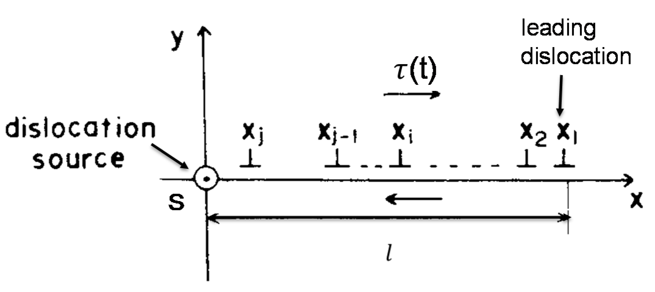
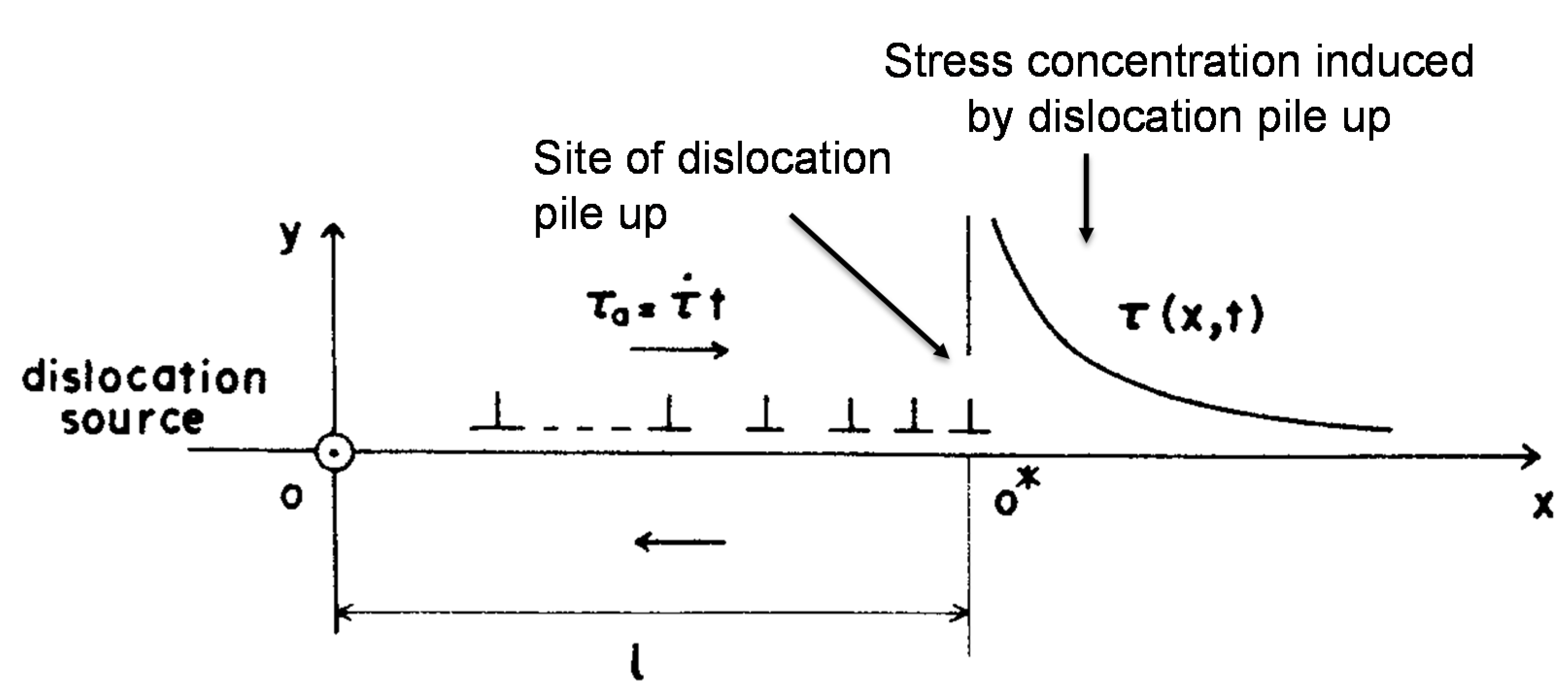
2.3. Dislocation Pile-Up Induced by Local Stress Field [2]

Some previous research has treated analyses of dislocation pile-up [4,11,15], but there has not been so much research that has considered the application to fracture mechanics description.

In this section, numerical analyses were conducted on the dynamic piling-up of discrete dislocations emitted from a stressed source and on the dynamic stress intensity factor caused by discrete moving dislocations in a pile-up.

2.3.1. Model, Basic Equation and Analysis [2]

Until the lead dislocation in the array arrives at a barrier, such as grain boundary, dislocations will emit from a stressed source and move freely except for the interactions between dislocations, as shown in Figure 1. Equations of the motion of dislocation groups are given by Equations (1) and (2). After the arrival of the lead dislocation at the barrier, it is locked and the trailing dislocations pile-up against the barrier, as shown in Figure 2.

Equations of effective stress exerted on each dislocation in the array for the case of dislocation group pile-up are given by Equation (13).

$${\tau }_{eff,i}=\dot{\tau }t+A(\frac{1}{x_i-l}+{{\displaystyle \sum }}_{\begin{array}{c}j=2\\ i\ne j\end{array}}^n\frac{1}{x_i-x_j})\mathrm{i}=1\text{~}\mathrm{n}$$

(13)

The equation of motion of each dislocation in the array is calculated by Equation (1).

The effective stress exerted on a dislocation source before and after the leading dislocation arrives at the site of pile-up is given by Equations (14a) and (14b), respectively.

$${\mathsf{\tau }}_{eff,s}=\dot{\dot{\tau }t-A{\displaystyle \sum }_{j=2}^n\frac{1}{x_j},(x_1<l)}$$

(14a)

$${\mathsf{\tau }}_{eff,s}=\dot{\tau }t-A(\frac{1}{l}+{\displaystyle {\displaystyle \sum }_{j=2}^{\dot{n}}}\frac{1}{x_j}),\left(x_1=l\right)$$

(14b)

The stress distribution, $\mathsf{\tau }\left(x,t\right)$, caused by dynamical piling up in the region of $x>l$ is shown in Figure 3 and is given by Equation (15).

$$\mathsf{\tau }\left(x,t\right)=\frac{A}{x-l}+A{\displaystyle \sum }_{i=2}^n\frac{1}{x-x_i}+\dot{\tau t}$$

(15)

The dynamic stress intensity factor caused by dislocation pile-up formation is given by Equations (2)–(16).

$$\mathrm{k}\left(t\right)\cong \sqrt{2\mathsf{\pi }\left(x-l\right)}\tau {\left(x,t\right)}_{l<x<l\left(1+\mathsf{\epsilon }\right)}$$

(16)

where $l\mathsf{\epsilon }$ is the small distance in which the stress distribution has the characteristic of

$$\raisebox{1ex}{$1$}\!\left/ \!\raisebox{-1ex}{$\sqrt{x^{*}}$}\right.\left(x^{*}=x-l=l\mathsf{\epsilon }\right)$$

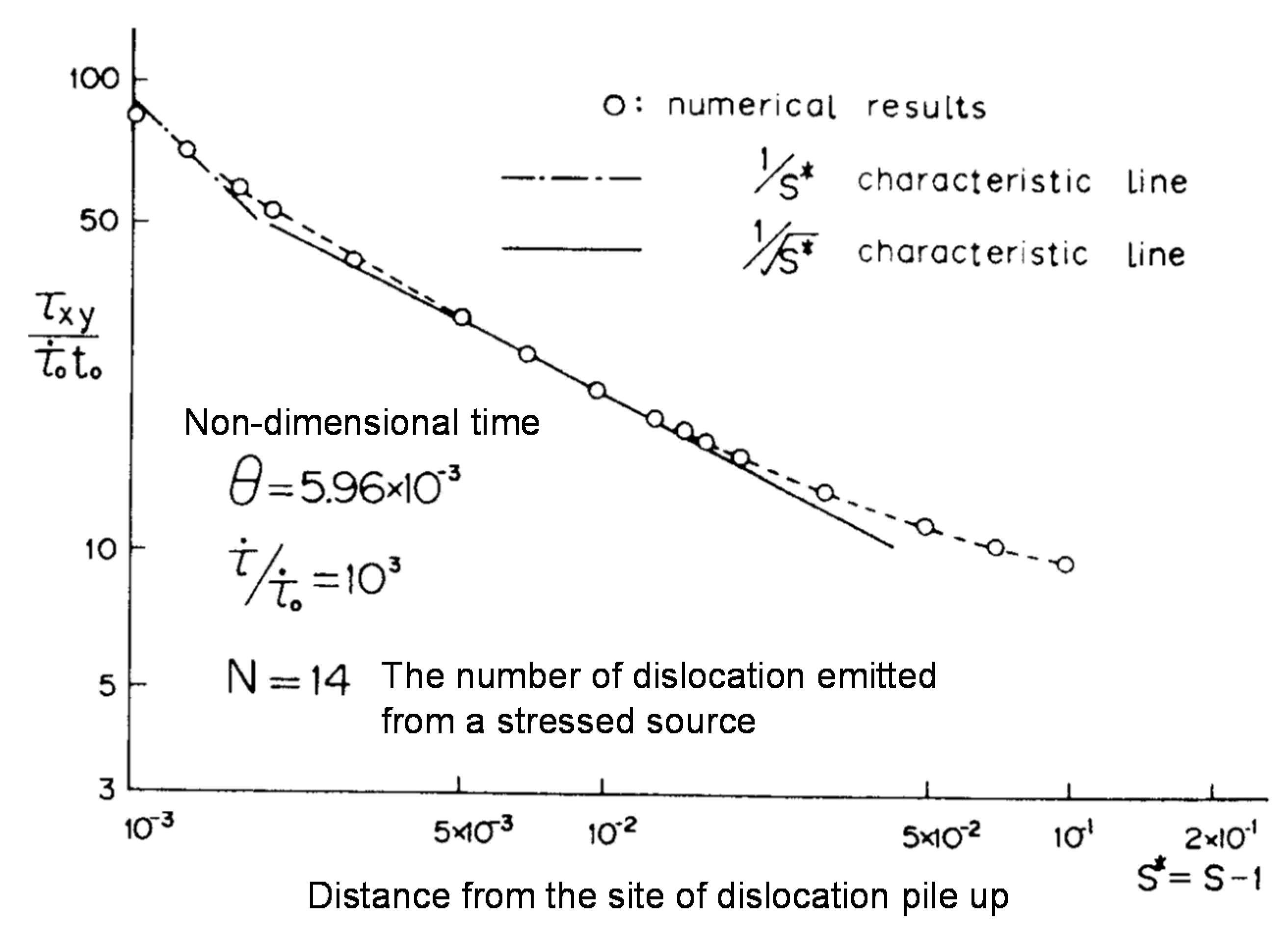
2.3.2. Results [2,3]

The numerical results of stress distribution on the slip line $\mathrm{x}>l$ near the site of pile-up (barrier) were obtained by Equation (15), as shown in Figure 4 and Figure 5, where s^* $=\mathrm{s}-1$ is the non-dimensional distance from the site of dislocation pile-up (O^* in Figure 3), S is the non-dimensional value of x controlled by $l$.

When the number of dislocations emitted is as small as shown in Figure 4, the stress distribution near the barrier shows a 1/s^* singularity, and with an increase in s*, a $\raisebox{1ex}{$1$}\!\left/ \!\raisebox{-1ex}{$\sqrt{s^{*}}$}\right.$ singularity appears but is restricted within a narrow region. ($3\times {10}^{-3}<s^{*}<2\times {10}^{-2})$ The characteristics of $\raisebox{1ex}{$1$}\!\left/ \!\raisebox{-1ex}{$\surd S^{*}$}\right.$ take minor portion in the stress distribution [2].

On the other hand, when the number of emitted dislocations increases, as shown in Figure 5 (sixty emitted dislocations), the stress distribution shows a singularity of $\raisebox{1ex}{$1$}\!\left/ \!\raisebox{-1ex}{$\sqrt{s^{*}}$}\right.$, which appears from the vicinity of the barrier; this characteristic region extends up to 5% of the length of slip line [2].

The numerical results of the dynamic stress intensity factor $\overline{K_d}\left(\mathsf{\theta }\right)$ due to pile-up by discrete dislocation groups dynamics with emission were obtained, as shown in Figure 6, by using Equations (15) and (16) and by the $\raisebox{1ex}{$1$}\!\left/ \!\raisebox{-1ex}{$\sqrt{s^{*}}$}\right.$ singularity of the stress distribution, as in Figure 5. A static solution, $\overline{K_s}\left(\mathsf{\theta }\right)$, obtained by the concept of continuously distributed infinitesimal dislocations for the equilibrium pile-up is given by Equation (17) and is also shown in Figure 6 for comparison with the dynamic stress intensity factor, $\overline{K_d}\left(\mathsf{\theta }\right)$. $\overline{K_s}\left(\mathsf{\theta }\right)$ and the linear part of $\overline{K_d}\left(\mathsf{\theta }\right)$ in Figure 6 are written as follows.

$$\overline{K_s}\left(\mathsf{\theta }\right)={10}^3\mathsf{\theta }$$

(17)

$$\overline{K_d}\left(\mathsf{\theta }\right)=1.2\times {10}^3\mathsf{\theta }-5.2$$

(18)

$$\mathrm{where}\mathsf{\theta }=\frac{t}{t_0}$$

The values of $\overline{K_d}\left(\mathsf{\theta }\right)$/$\overline{K_s}\left(\mathsf{\theta }\right)$ were plotted against non-dimensional time, $\mathsf{\theta }$, as shown in Figure 7. From these results, it can be seen that the dynamic stress intensity factor is smaller than the static one and asymptotically approaches the static one as the number of emitted dislocations increases.

The calculated dynamic dislocation density distribution $f_d$ is shown in Figure 8, Figure 9, Figure 10 and Figure 11 [3]. On the other hand, the static dislocation density distribution $f_s$ and the number of dislocations N under equilibrium state without emitting are given by the continuous distributed infinitesimal dislocations concept, assuming $f_s\left(s\right)=0$ at the dislocation source and $f_s\left(s\right)\to \infty$ at the site of pile-up, respectively. They are given by Equations (19) and (20).

$$f_s\left(s\right)=\frac{{\tau }_a}{\mathsf{\pi }{A}^{*}}\sqrt{\frac{s}{1-s}}$$

(19)

$$\mathrm{N}={{\displaystyle \int }}_0^d{f}_s\left(s\right)ds=\frac{{\mathsf{\tau }}_{a}d}{2A^{*}}$$

(20)

In Figure 8, Figure 9, Figure 10 and Figure 11, $f_s$ is shown by the dotted line. These results showed when the stress application rate, $\dot{\tau }$, or grain size, d, is small, and a static equilibrium solution based on a continuous distribution of infinitesimal dislocations gives a good approximation, as shown in Figure 8 and Figure 9. However, with increase in $\dot{\tau }$ or d, the dynamic effect becomes more remarkable and $f_d$ becomes smaller than $f_s$ [3], as shown in Figure 10 and Figure 11 [3].

The dynamic stress intensity factor $\overline{K_d}\left(\mathsf{\theta }\right)$ at the site of pile-up such as grain boundary in non-dimensional form can be obtained using Equation (16). In Figure 12, $\overline{K_d}\left(\mathsf{\theta }\right)$/$\overline{K_s}\left(\mathsf{\theta }\right)$ is plotted against the non-dimensional dynamic factor $\mathsf{\Theta }={\left(\raisebox{1ex}{$\dot{\tau }$}\!\left/ \!\raisebox{-1ex}{${\dot{\tau }}_0$}\right.\right)}^{\raisebox{1ex}{$\left(m+1\right)$}\!\left/ \!\raisebox{-1ex}{$\left(m+2\right)$}\right.}\theta$ [9,10]. For the case of iron (m = 3 [13]), the following equation was obtained [3].

$$\frac{K_d}{K_s}=1.0-Aexp\left(-B\Theta \right)$$

(21)

By using the non-linear least square method, A and B in Equation (21) were obtained as a function of $\raisebox{1ex}{$\dot{\tau }$}\!\left/ \!\raisebox{-1ex}{${\dot{\tau }}_0$}\right.$ and d, respectively, as follows [3].

$$\mathrm{A}=\mathsf{\phi }\left(\frac{\dot{\tau }}{{\dot{\tau }}_0},d\right)=2.35-0.0214{\left(\frac{\dot{\tau }}{{\dot{\tau }}_0}\right)}^{-0.172}{d}^{-0.896}$$

(22)

$$\mathrm{B}=\mathsf{\psi }\left(\frac{\dot{\tau }}{{\dot{\tau }}_0},d\right)=1.08{\left(\frac{\dot{\tau }}{{\dot{\tau }}_0}\right)}^{-0.0557}$$

(23)

The results of Figure 13 and Figure 14 show that Equations (22) and (23) well-represent numerical results.

By substituting Equations (22) and (23) into Equation (21), Equation (24) can be obtained [3].

$$\frac{K_d}{K_s}=1.0-\left\{2.35-0.0214{\left(\frac{\dot{\tau }}{{\dot{\tau }}_0}\right)}^{-0.172}{d}^{-0.896}\right\}exp\left\{-1.08{\left(\frac{\dot{\tau }}{{\dot{\tau }}_0}\right)}^{0.75}\frac{t}{t_0}\right\}$$

(24)

Figure 15 shows that the calculated values from Equation (24) were found to be in good agreement with data obtained by numerical analyses.

By using dimensional analysis and determining the coefficient of the constant term using the number of material constants, Equation (24) leads to Equation (25) [3].

$$K_d\left(t\right)=\sqrt{2\mathsf{\pi }\mathrm{d}}\left(\dot{\tau }t\right)\left[\begin{array}{c}1.0-\left\{2.35-0.230{\left(\frac{G}{{\tau }_0^{*}}\right)}^{\raisebox{1ex}{$m$}\!\left/ \!\raisebox{-1ex}{$\left(m+2\right)$}\right.}{\left(\frac{G{V}_0}{\dot{\tau }b}\right)}^{\raisebox{1ex}{$1$}\!\left/ \!\raisebox{-1ex}{$\left(m+2\right)$}\right.}{\left(\frac{b}{d}\right)}^{\raisebox{1ex}{$\left(m+1\right)$}\!\left/ \!\raisebox{-1ex}{$\left(m+2\right)$}\right.}\right\}\\ \times exp\left\{-1.08{\left(\frac{\dot{\tau }t}{{\tau }_0^{*}}\right)}^{\raisebox{1ex}{$m$}\!\left/ \!\raisebox{-1ex}{$\left(m+2\right)$}\right.}{\left(\frac{V_{0}t}{\left(m+1\right)d}\right)}^{\raisebox{1ex}{$1$}\!\left/ \!\raisebox{-1ex}{$\left(m+1\right)$}\right.}\right\}\end{array}\right]$$

(25)

2.4. Application to Problem of Yielding

2.4.1. Basic Equations

Cottrell and Bilby described the mechanism of yielding from the view point of dislocation trapping mechanism by solute atoms of carbon [7]; however, the effect of strain rate and temperature have not yet been fully formulized. Concerning ductile fracture of steels, the formulation of the upper yielding point and delay time for yielding are important factors to be analyzed. Takeo Yokobori conducted the formulation of the stress rate dependence of the upper yield point based on a stochastic model analysis that analyzed the releasing process of solute atom from a dislocation [8].

On the other hand, on the basis of the concept that the velocity of an isolated dislocation is proportional to the strain rate of a specimen given by Equation (26), Johnson [15] and Hahn [16] described the yielding phenomenon from the view point of theory of dislocation [15,16]. However, a cleared formulation of yielding phenomenon including the effect of temperature has not yet been conducted. Furthermore, the researchers used the equation of velocity of an isolated dislocation motion by considering that every dislocation moves at the same velocity without interaction between them, as given by Equation (26) [16].

$$\dot{\gamma }=\rho b\overline{v}$$

(26)

In the equation, $\rho$ is the dislocation density, b is the Burgers vector, and $\overline{v}$ is the mean velocity of a dislocation in which the equation of velocity of an isolated dislocation was used.

In this section, instead of Equation (26), Equation (27) [4,17], which considers the interaction of dislocations within groups starting with dislocation emission from a stressed source (as calculated by Equations (1) and (2)) was adopted.

$$\dot{\gamma }=\rho b{\displaystyle \sum }_{i=1}^{n\left(t\right)}{v}_i$$

(27)

In Equation (27), n(t) is the number of dislocations emitted from a stressed source at the time of t, i is the dislocate-ion number, and $v_i$ is the velocity of the i th dislocation in the dislocation groups.

By conducting computer simulation using the physical model of Figure 1 and Equations (1)–(4), the summation of non-dimensional velocity of each dislocation in the array was found to be written by Equation (28) and is shown in Figure 16 [17].

$${\displaystyle \sum }_{i=1}^n\frac{v_i\left(t\right)}{v_{iso}}\cong n\left(t\right)$$

(28)

By substituting Equation (28) into Equation (27) and using Equation (29), the plastic strain rate is given by Equation (30) [17].

$$\rho ={\rho }_0^{*}{\Lambda }^{*}$$

(29)

In Equation (29), $\rho$ is the area density dislocation, ${\rho }_0^{*}$ is the volume density dislocation, and ${\Lambda }^{*}$ is the average length of dislocation.

$$\dot{\gamma }={\rho }_0^{*}{\Lambda }^{*}bn\left(t\right)v_0{\left(\frac{\tau }{{\tau }_0}\right)}^m=\overline{\rho }\left(t\right)bv$$

(30)

In Equation (30), $\overline{\rho }\left(t\right)={\rho }_0^{*}{\Lambda }^{*}n\left(t\right)$, and $v$ is given by Equation (3).

2.4.2. The Application of This Theory to Yielding of Steels

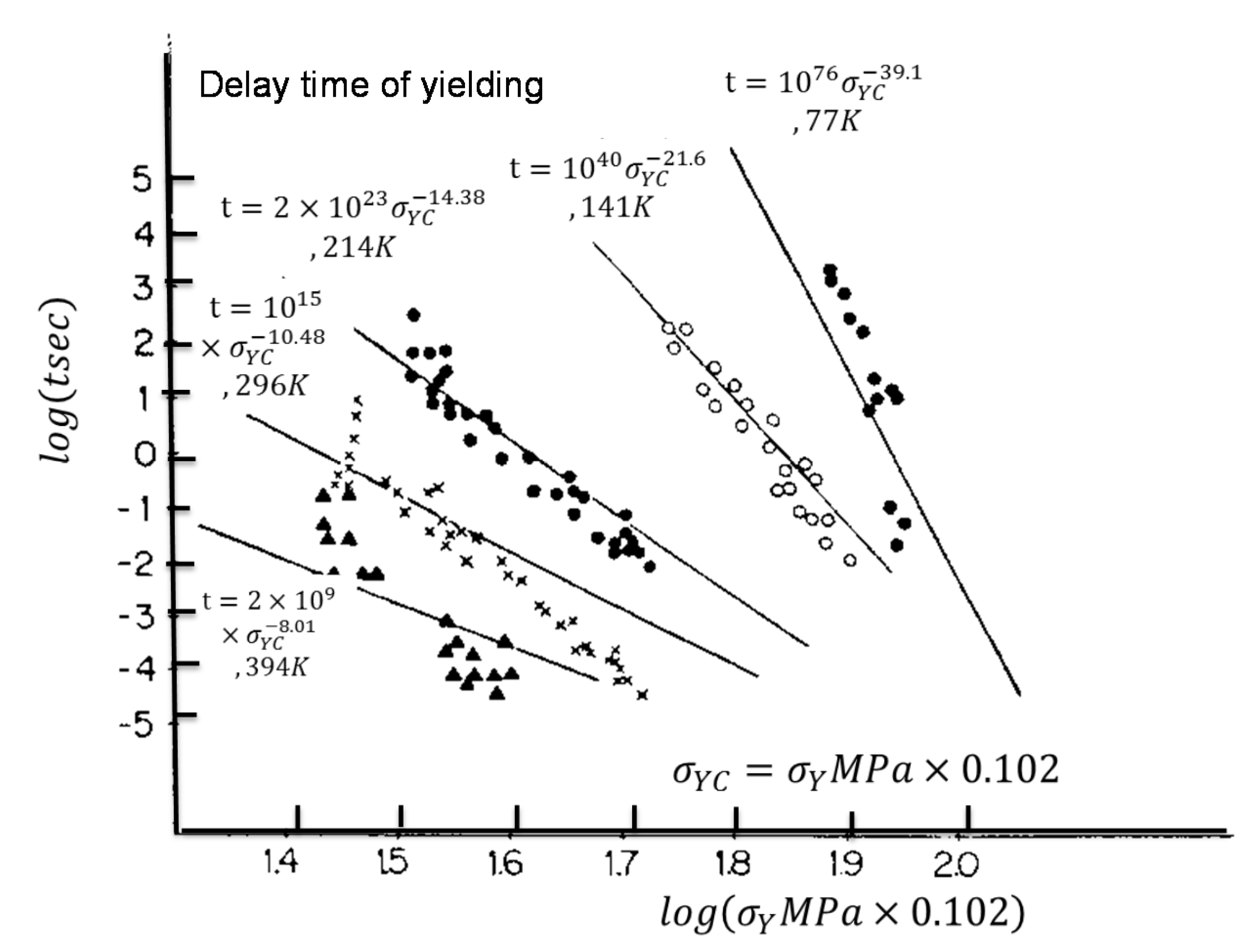
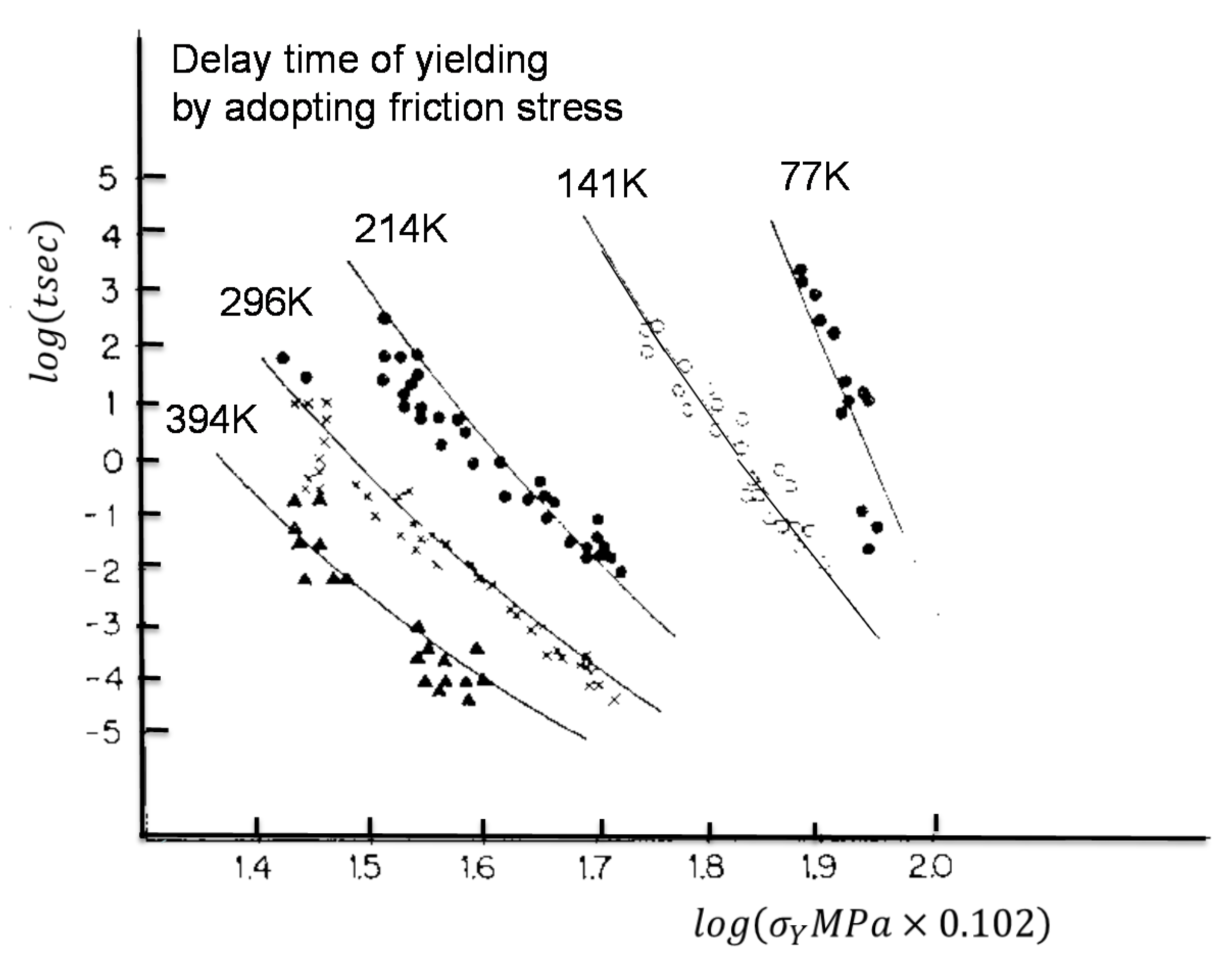
The Delay Time of Yielding

The delay time of yielding under rapid application of constant stress is calculated by Equation (31) as the time of plastic strain, thus taking the specified value [16].

$${\gamma }_P={{\displaystyle \int }}_0^t\dot{\gamma }dt=const$$

(31)

Using Equations (30) and (32), which are the number of dislocations emitted from a stressed source under constant stress condition [6], and by substituting Equations (30) and (32) into Equation (31) and integrating Equation (31), Equation (33) was obtained [17].

$$\mathrm{n}\left(\mathrm{t}\right)=2.45m^{-0.865}{\left(\frac{b}{v_{0}t}\right)}^{-\raisebox{1ex}{$\left(m+1\right)$}\!\left/ \!\raisebox{-1ex}{$\left(m+2\right)$}\right.}{\left(\frac{{\tau }_0^{*}}{G}\right)}^{-\raisebox{1ex}{$m\left(m+1\right)$}\!\left/ \!\raisebox{-1ex}{$\left(m+2\right)$}\right.}{\left(\frac{{\tau }_a}{G}\right)}^{\raisebox{1ex}{${\left(m+1\right)}^2$}\!\left/ \!\raisebox{-1ex}{$\left(m+2\right)$}\right.}$$

(32)

where G is the shear modulus. ${\tau }_a={\tau }_Y=\raisebox{1ex}{${\sigma }_Y$}\!\left/ \!\raisebox{-1ex}{$2$}\right.$, where ${\sigma }_Y$ is the yield stress under uniaxial tensile load, is assumed.

$$\mathrm{t}={\left(\frac{{\gamma }_P}{{\rho }_0^{*}\Lambda b^2}\frac{2m+3}{m+2}\frac{m^{0.865}}{2.45}\right)}^{\frac{m+2}{2m+3}}\frac{b}{v_0}{\left(\frac{G}{{\tau }_0^{*}}\right)}^{\frac{m+1}{2m+3}}{\left(\frac{{\sigma }_Y}{2{\tau }_0^{*}}\right)}^{-\frac{\left(2m^2+4m+1\right)}{\left(2m+3\right)}}$$

(33)

By using Equations (7)–(10), Equation (33) was able to be written in the following manner as a function of yield stress, temperature, and material constants [17].

$$\mathrm{t}={\left(\frac{0.792{\gamma }_P}{{\rho }_0^{*}\Lambda b^2}\right)}^{0.515}{\left(\frac{H_k}{4kT}\right)}^{0.446}\frac{b}{A_1}{\left(\frac{G}{{\tau }_{00}}\right)}^{0.485}{\left(\frac{{\sigma }_Y}{2{\tau }_{00}}\right)}^{-\left(\raisebox{1ex}{$H_k$}\!\left/ \!\raisebox{-1ex}{$4kT$}\right.\right)}$$

(34)

In Equation (34), ${\sigma }_Y$ is the yield stress under uniaxial tensile loading. As the criterion of yielding, ${\gamma }_p=0.01$ and ${\rho }_0^{*}{\Lambda }^{*}={10}^8/m^2$ were selected [15], and G = 79.38 GPa, ${\tau }_0^{*}=169.6\mathrm{MPa}$ [10], m = 10 [16] were taken as those under room temperature and $\mathrm{b}=3\times {10}^{-10}m$ was selected. Furthermore, for m = 10~30 (for steel) [13], $\left(2m^2+4m+1\right)/\left(2m+3\right)\approx m$ was approximately assumed.

A comparison of Equation (34) with experimental data is shown in Figure 17 [17]. Equation (34) was found to well-predict experimental data [18,19]. Furthermore, this equation was in good agreement with that obtained based on dislocation dynamics theory that defined yielding to occur when the dislocation density takes some critical value [6] as follows.

$$\mathrm{t}={\left(\frac{\overline{N_0}}{{\rho }_0^{*}\Lambda 2.45}\right)}^{1.06}{\left(\frac{H_k}{4kT}\right)}^{0.917}\frac{b}{A_1}\left(\frac{G}{{\tau }_{00}}\right){\left(\frac{{\sigma }_Y}{2{\tau }_{00}}\right)}^{-\left(\raisebox{1ex}{$H_k$}\!\left/ \!\raisebox{-1ex}{$4kT$}\right.\right)}$$

(35)

In Equation (35), $\overline{N_0}$ is critical dislocation density at the yielding.

This means that the ${\gamma }_P$ criterion is identical to the $\overline{N_0}$ criterion.

Furthermore, Equation (34) was found to be in good qualitative agreement with theoretical results [8] based on Cottrell-Bilby’s dislocation release mechanism [7] for locking by solute atoms such as carbon or nitrogen, as given by Equation (36). This means that the locking mechanism closely connects with the mechanism of dislocation group dynamics, as described in the following expression.

$$\mathrm{t}=t_0{\left(\frac{{\sigma }_Y}{{\sigma }_0}\right)}^{-\raisebox{1ex}{$1$}\!\left/ \!\raisebox{-1ex}{$nkT$}\right.}$$

(36)

where t₀ and ${\sigma }_0$ are material constants.

T. Yokobori found that adopting a friction stress, ${\tau }_i$, to resist the motion of a dislocation in Equation (36) was very effective in obtaining agreement with experimental results via equations [20]. In this theory, the effect of ${\tau }_i$ on delay time for yielding, as included in Equation (33), was extended to then give Equation (37) [17].

$$\mathrm{t}={\left(\frac{{\gamma }_P}{{\rho }_0^{*}\Lambda b^2}\frac{2m+3}{m+2}\frac{m^{0.865}}{2.45}\right)}^{\frac{m+2}{2m+3}}\frac{b}{v_0}{\left(\frac{G}{{\tau }_0^{*}-{\tau }_i}\right)}^{\frac{m+1}{2m+3}}{\left(\frac{{\sigma }_Y}{2\left({\tau }_0^{*}-{\tau }_i\right)}\right)}^{-\frac{\left(2m^2+4m+1\right)}{\left(2m+3\right)}}$$

(37)

By adopting ${\tau }_i=86.3\mathrm{MPa}$ and using Equations (10a)–(10d), Equation (37) was found to well-predict experimental results [19], as shown in Figure 18 [17].

Furthermore, a previous numerical analysis based on the pile-up behaviors of moving dislocations emitted from a stressed source was conducted [4], and the theoretical relationship between delay time of yielding and yield stress was derived for various grain size [4]. These results were found to be in good agreement with experimental results and were also found to produce similar characteristics to the results given by Figure 18 [17].

From the results mentioned above, the criteria for the various cases of dislocation release from locking by solute atom [8], critical plastic strain [16,17], critical dislocation density [6], and dislocation pile-up at the grain boundary [4] were closely associated with the sequential processes involved in determining the delay time for yielding. Thus, the theoretical results [8] based on Cottrell-Bilby’s dislocation release mechanism [7] for dislocation locking by solute atoms (Equation (36)) are considered to be the starting for understanding plastic yielding.

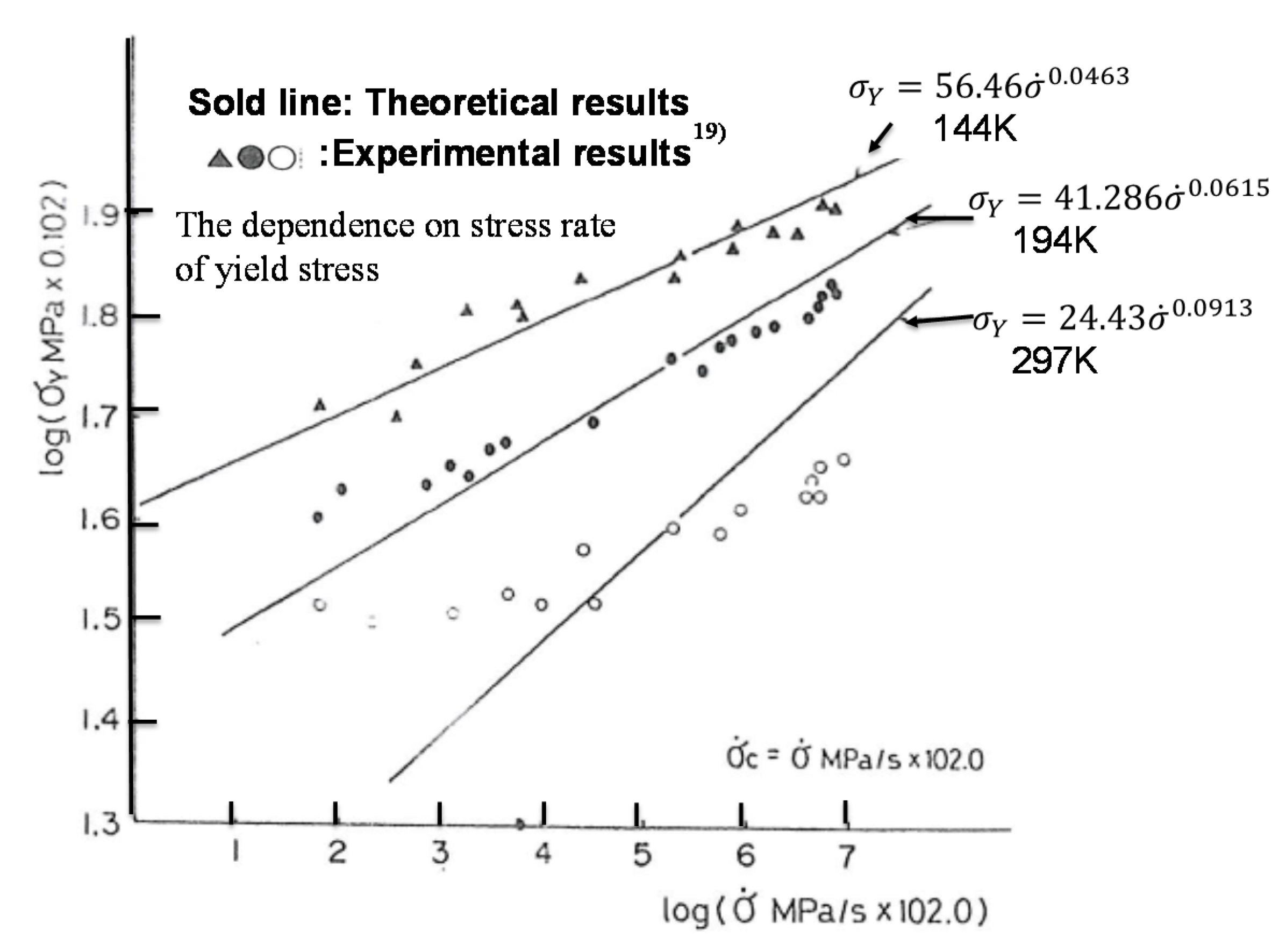
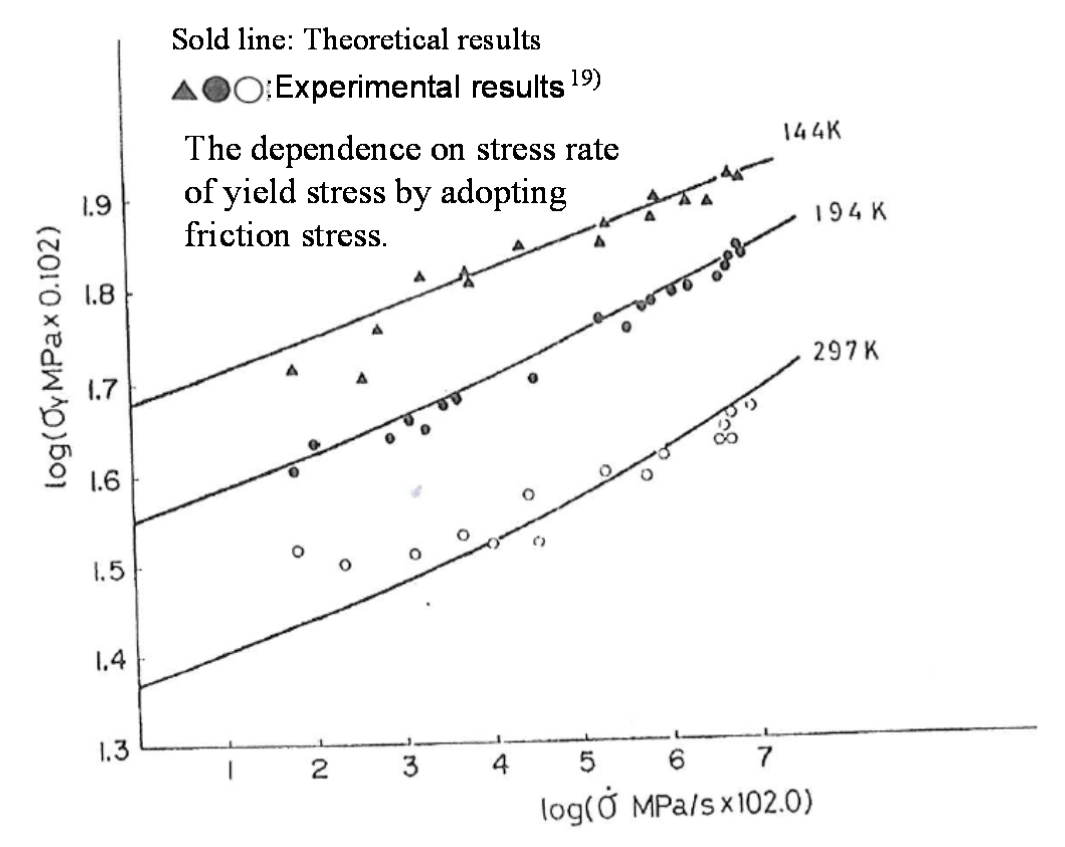
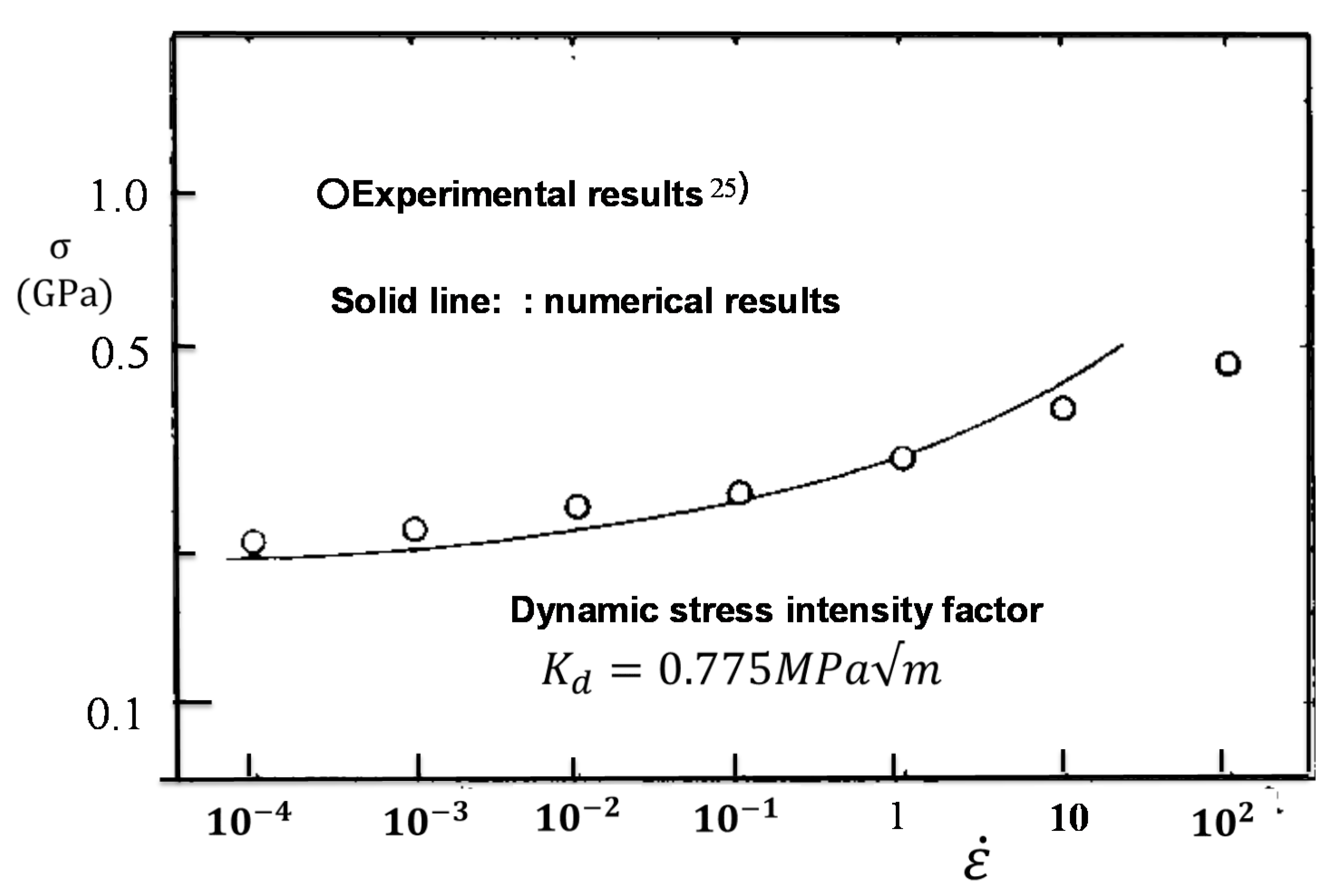
The Applied Stress Rate Dependence of Yield Stress [17]

Strain rate caused by applied stress, $\dot{{\gamma }_a}$, is given by the summation of plastic strain rate of the specimen, $\acute{{\gamma }_P}$, and elastic strain rate including those of grips and rigidity of testing machine, $\dot{{\gamma }_e}$, as follows.

$$\dot{{\gamma }_a}=\acute{{\gamma }_e}+\dot{{\gamma }_P}$$

(38)

For the case of a sharp yielding point, $\dot{{\gamma }_e}\approx 0$ is satisfied at the yield point. Therefore, $\dot{{\gamma }_a}$ is given by Equation (39).

$$\dot{{\gamma }_a}=\dot{{\gamma }_P}\approx A^{*}\frac{1}{G}\dot{{\tau }_a}$$

(39)

where A^* is a proportional constant. By using Equations (11) and (12) for the number of dislocations emitted from a stressed source under constant stress rate condition and then substituting Equations (26) and (27) into Equation (39), ${\sigma }_Y$ can be given by Equation (40) as a function of stress rate and material constants. Furthermore, ${\tau }_a={\tau }_Y=\raisebox{1ex}{${\sigma }_Y$}\!\left/ \!\raisebox{-1ex}{$2$}\right.$ and $\acute{\tau }=\frac{\acute{\sigma }}{2}$ were also assumed.

$${\sigma }_Y=2{\tau }_0^{*}{\left(\frac{m^{1.45}}{1.4}\frac{A^{*}}{{\rho }_0^{*}\Lambda b^2}\right)}^{\raisebox{1ex}{$1$}\!\left/ \!\raisebox{-1ex}{$\left(2m+1\right)$}\right.}{\left(\frac{{\tau }_0^{*}}{G}\right)}^{-\raisebox{1ex}{$2\left(m+1\right)$}\!\left/ \!\raisebox{-1ex}{$\left(m+2\right)\left(2m+1\right)$}\right.}{\left(\frac{\acute{\sigma }b}{2v_{0}G}\right)}^{\frac{\left(2m+3\right)}{\left(m+1\right)\left(2m+1\right)}}$$

(40)

Using Equations (7)~(10) and the following approximation for m = 10–30 (steel) [16], Equation (42) was obtained.

$$\frac{2m+1}{\left(m+2\right)\left(2m+1\right)}\approx \frac{1}{m+2}\approx \frac{1}{m+1}\approx \frac{1}{m}$$

(41)

$${\sigma }_Y=2{\tau }_{00}{\left\{\frac{A^{*}}{1.4}{\left(\frac{H_k}{4kT}\right)}^{1.45}\frac{1}{{\rho }_0^{*}\Lambda b^2}{\left(\frac{{\tau }_{00}}{G}\right)}^{-1.9}\right\}}^{\raisebox{1ex}{$2kT$}\!\left/ \!\raisebox{-1ex}{$H_k$}\right.}{\left(\frac{\acute{\sigma }b}{2A_{1}G}\right)}^{\raisebox{1ex}{$4kT$}\!\left/ \!\raisebox{-1ex}{$H_k$}\right.}$$

(42)

As material constants, the following physically reasonable and almost equal values to those used for the analysis of the delay time of yielding, ${\rho }_0^{*}\Lambda =1.75\times {10}^6/{\mathrm{m}}^2$ [16], G = 79.38 GPa, ${\tau }_0^{*}=176.0\mathrm{MPa}$ [18], and m = 10 [16] were taken at room temperature, with $b=3\times {10}^{-10}\mathrm{m}$ selected. Before yielding, since ${\tau }_a=G{\gamma }_a$ was almost satisfied, $A^{*}$ was considered to be almost equal to one.

A comparison of Equation (42) with experimental data is shown in Figure 19 [17]. Equation (42) was found to agree well with experimental data [19]. Furthermore, this equation was in good agreement with that obtained based on dislocation dynamics theory that defined yielding as occurring when dislocation density takes some critical value [6] as follows.

$${\sigma }_Y=2{\tau }_{00}{\left\{\frac{1}{1.4}{\left(\frac{H_k}{4kT}\right)}^{1.45}\frac{\overline{N_0}}{{\rho }_0^{*}\Lambda }\right\}}^{\raisebox{1ex}{$4kT$}\!\left/ \!\raisebox{-1ex}{$H_k$}\right.}{\left(\frac{G\acute{\sigma }b}{2A_1{\tau }_{00}^2}\right)}^{\raisebox{1ex}{$4kT$}\!\left/ \!\raisebox{-1ex}{$H_k$}\right.}$$

(43)

This means that the ${\gamma }_P$ criterion is identical to the $\overline{N_0}$ criterion. Furthermore, Equation (42) was found to be in in good qualitative agreement with theoretical results [8] based on Cottrell-Bilby’s dislocation release mechanism [7] for dislocation locking by solute atoms such as carbon or nitrogen, as given by Equation (44). This means that the locking mechanism closely connects with the mechanism of dislocation group dynamics as the appropriate mechanism of locking.

$${\sigma }_Y={\sigma }_0{\left(\frac{t_0}{nkT}\frac{\acute{\sigma }}{{\sigma }_0}\right)}^{nkT}$$

(44)

Furthermore, other results obtained based on a viscoplasticity model also showed the same type of relationship between strain rate and yield stress [5].

From the total results mentioned above, it can be seen the criteria of dislocation release from locking by the solute atom [8], critical strain rate [16,17], critical dislocation density [6], and viscoplasticity [5] are closely connected with the sequential processes of plastic yielding. Furthermore, the theoretical results [8] based on Cottrell-Bilby’s dislocation release mechanism [7] from locking by solute atom (Equation (44)) are considered to be a starting process of yielding.

T. Yokobori also found that the adoption of the friction stress, ${\tau }_i$, of the motion of dislocation in Equation (40) was very effective in predicting experimental results with the current equation [20]. In this theory for Equation (40), the effect of ${\tau }_i$ on yield stress carries on to lead to Equation (45) [17].

$${\sigma }_Y={\sigma }_i+2\left({\tau }_0^{*}-{\tau }_i\right){\left(\frac{m^{1.45}}{1.4}\frac{A^{*}}{{\rho }_0^{*}\Lambda b^2}\right)}^{\raisebox{1ex}{$1$}\!\left/ \!\raisebox{-1ex}{$\left(2m+1\right)$}\right.}{\left(\frac{{\tau }_0^{*}-{\tau }_i}{G}\right)}^{-\raisebox{1ex}{$2\left(m+1\right)$}\!\left/ \!\raisebox{-1ex}{$\left(m+2\right)\left(2m+1\right)$}\right.}{\left(\frac{\acute{\sigma }b}{2v_{0}G}\right)}^{\frac{\left(2m+3\right)}{\left(m+1\right)\left(2m+1\right)}}$$

(45)

By adopting ${\tau }_i=86.3\mathrm{MPa}$ and using Equations (10a)–(10d), Equation (45) was found to well-predict experimental results [19], as shown in Figure 20 [17].

The relationship between ${\tau }_0^{*}$ used for analyses of Figure 17, Figure 18, Figure 19 and Figure 20 and temperature T is shown in Figure 21. The results were in good agreement with the theoretical relationship given by Equation (10c), thus showing the validity of the method of analysis.

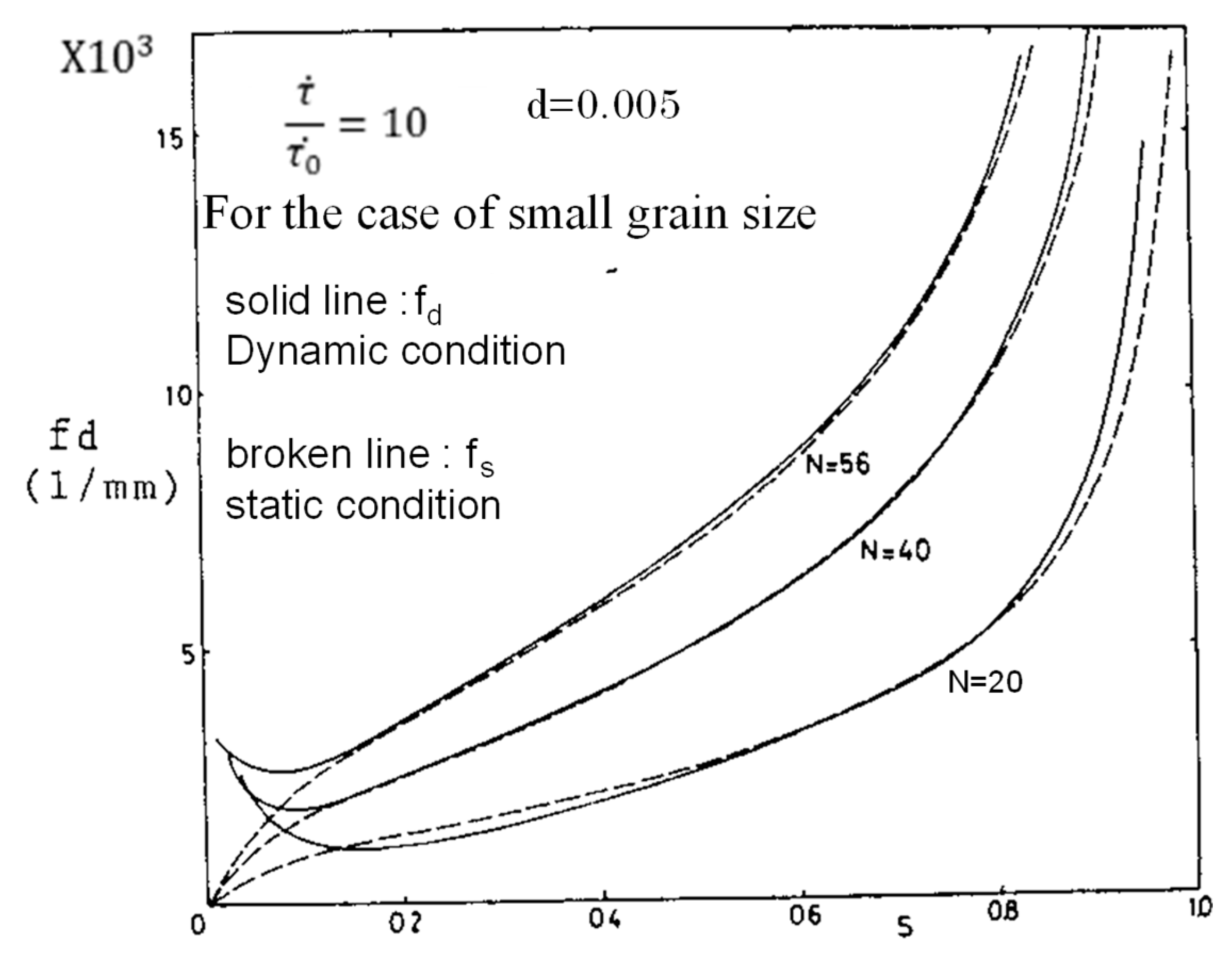
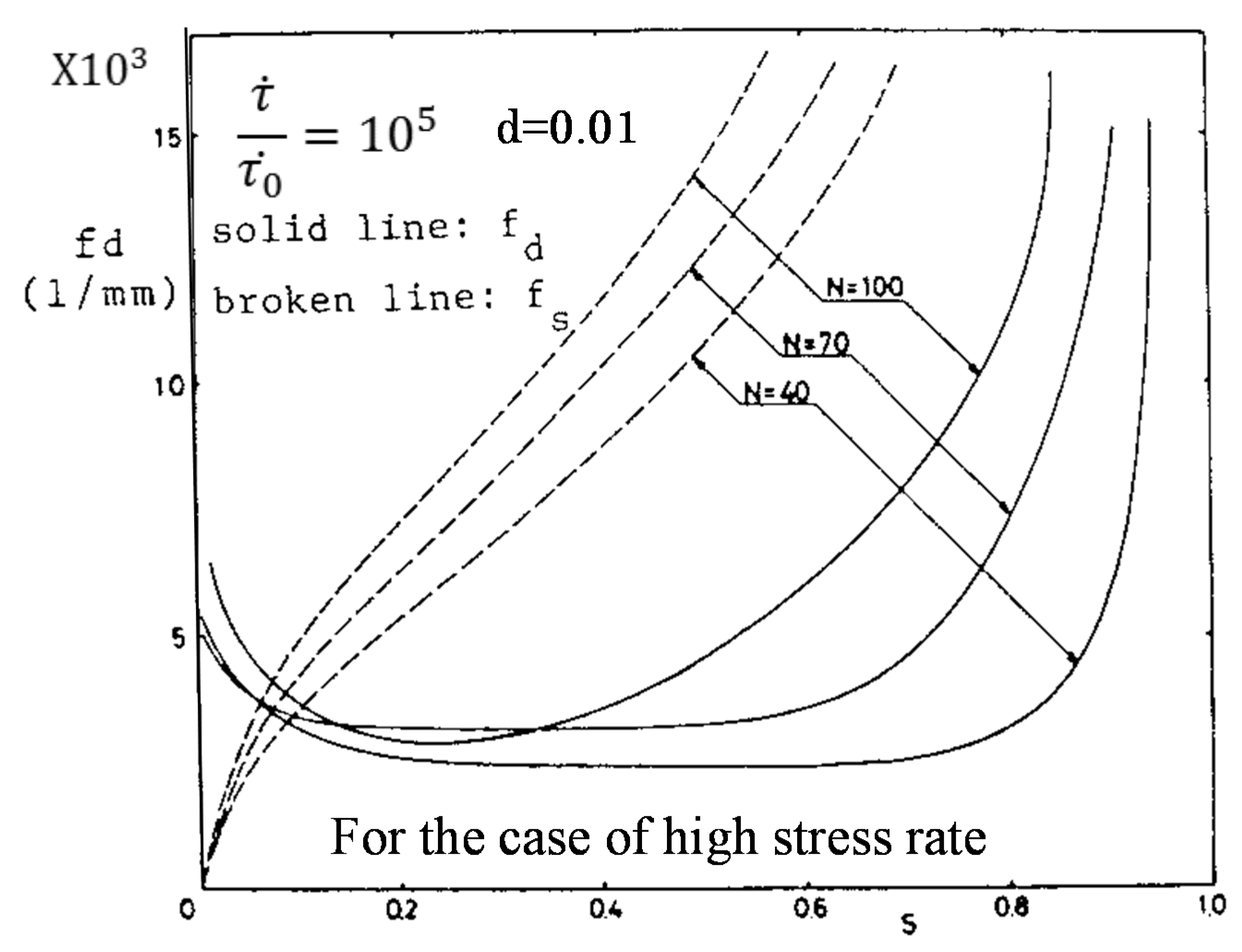
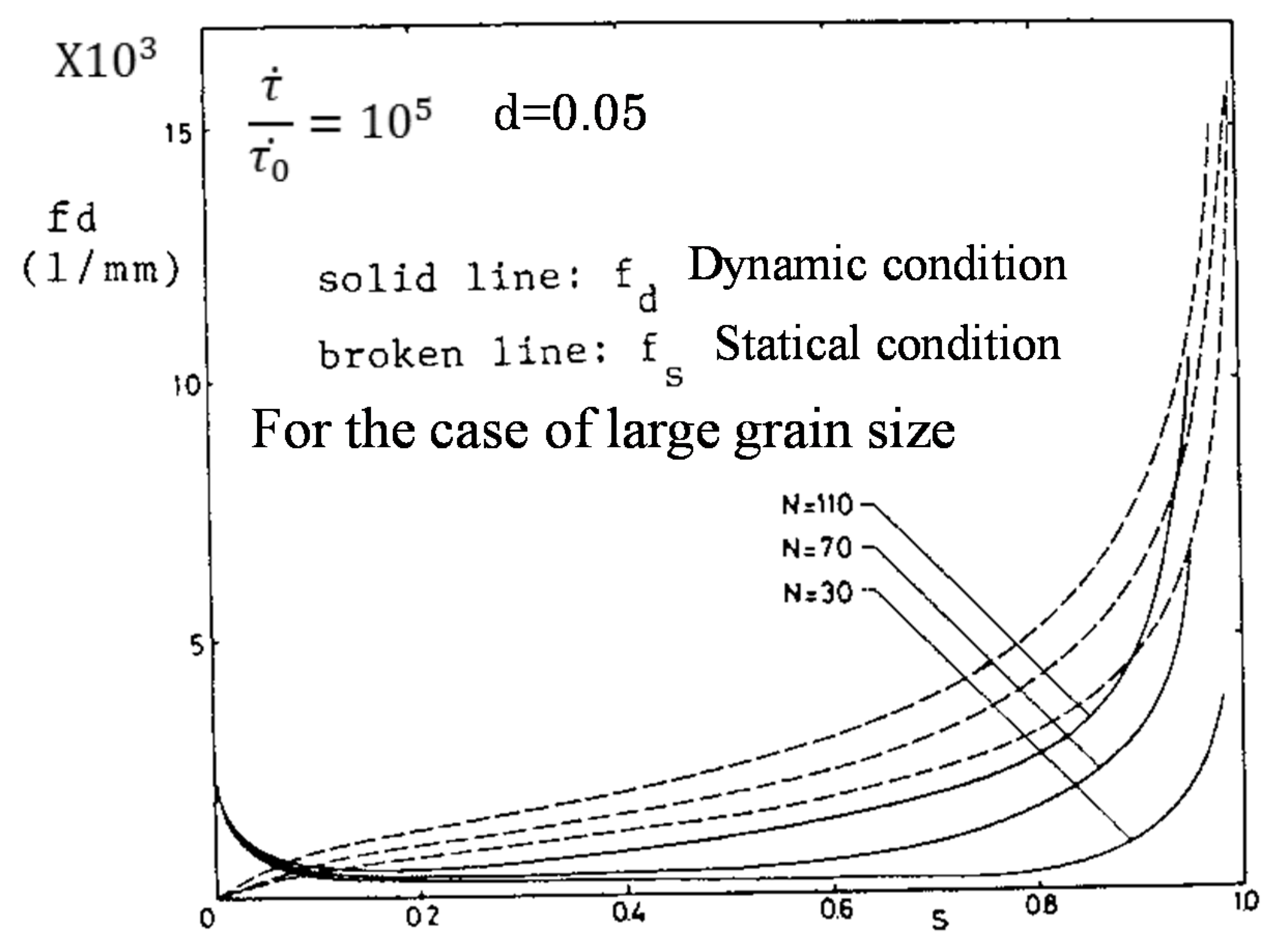
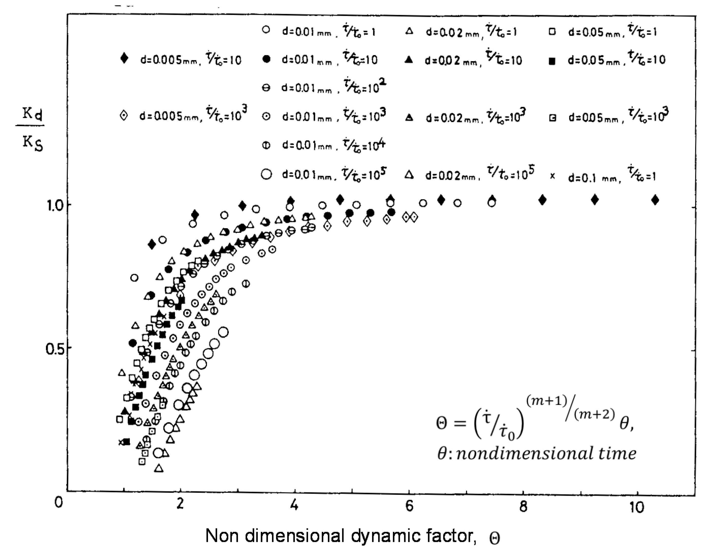
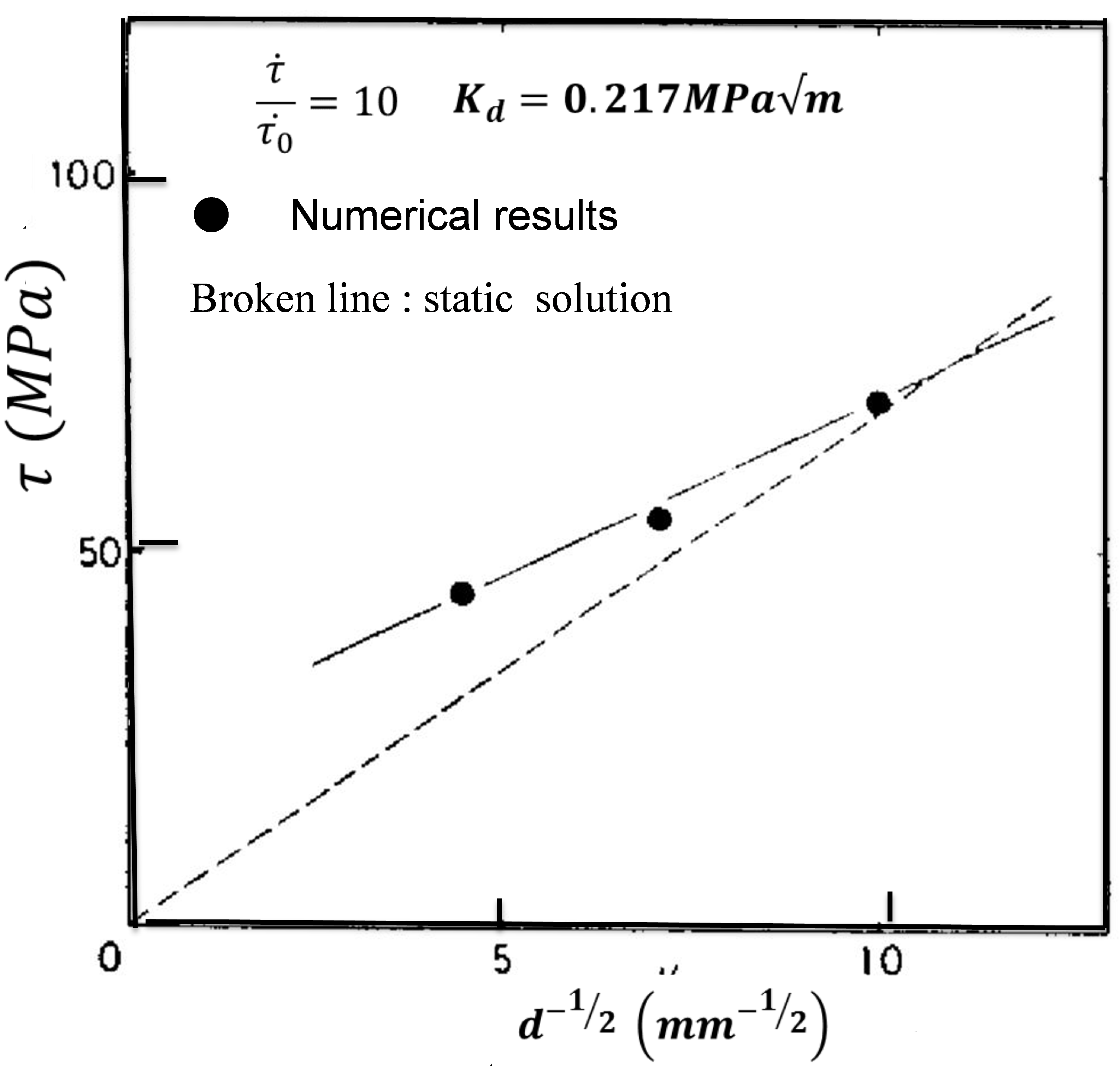
The Effect of Grain Size and Applied Strain Rate on Yield Stress Based on the Theory of Dislocation Piling Up [2,3,21]

The effect of grain size d on lower yield point was obtained by the following experimental relationship [22,23].

$${\sigma }_{l,y}={\sigma }_s+\kappa d^{\raisebox{1ex}{$-1$}\!\left/ \!\raisebox{-1ex}{$2$}\right.}$$

(46)

where ${\sigma }_s$ and κ are material constants that are positive values.

Furthermore, many detailed studies have been conducted on this relationship [24,25].

In this section, using the Equation (25), the calculated relationship between an applied stress, $\mathsf{\tau }$, required for a dynamic $K_d$ to take on a critical value over a range in grain size d is shown by the solid line in Figure 22 [3], which is expressed by Equation (47).

$$\mathsf{\tau }={\tau }_1+k\frac{1}{\sqrt{d}}$$

(47)

where ${\tau }_1$ and $k$ are constants. The dashed line is a static solution given by Equation (48).

$$\mathsf{\tau }=\frac{K_s}{\sqrt{2\pi d}}$$

(48)

where $K_s$ is static stress intensity factor.

It can be seen from Equation (47) that the dynamic yield strength also increases linearly with respect to the inverse square root of grain size. Furthermore, by comparing Equations (47) and (48), the yield stress corresponding to $d^{-\raisebox{1ex}{$1$}\!\left/ \!\raisebox{-1ex}{$2$}\right.}\approx 0$ was found to be higher in dynamic yielding than that in the static case, and this characteristic is in good agreement with the experimental data [26].

Concerning the effect of applied strain rate on yield stress, the rate-determining process of yielding of iron and steel is considered to correspond to the dynamic piling up of emitted dislocations.

The dislocation pile-up at grain boundaries and yielding is considered to occur when $K_d$, given by Equation (25) to measure the local stress concentration, takes on a critical value. A comparison of results obtained by Equation (25) and experimental data [27] is shown in Figure 23 [3]. In Figure 23, the solid line represents the calculated relation between the applied stress $\mathsf{\sigma }$ required for $K_d$ to take the critical value and applied strain rate that is in good agreement with experimental data [25]. In Figure 23, $\acute{\epsilon }$ is evaluated by the relationship of $\acute{\sigma }=2\acute{\tau }=E\acute{\epsilon }$.

From the total results presented in Section 2.4, it can be seen that the various criteria associated with dislocation release from locking by solute atom [8]_, critical plastic strain [16,17], critical strain rate or stress rate, critical dislocation density [6], viscoplasticity [5], and dislocation pile-up at a grain boundary [3,4] characterized by local stress intensity factor [3] ($K_d$) all relate closely to the sequential processes of yielding. Furthermore, the theoretical results [8] based on Cottrell-Bilby’s dislocation release mechanism [7] for dislocation locking by solute atoms is considered to be a starting process of yielding.

In addition to the relationship between yield stress and grain size, a theoretical relationship between the yield stress and temperature was derived based on dislocation mechanics [28,29]. The present description closely connects with the results given in Figure 18 and Figure 20 [17].

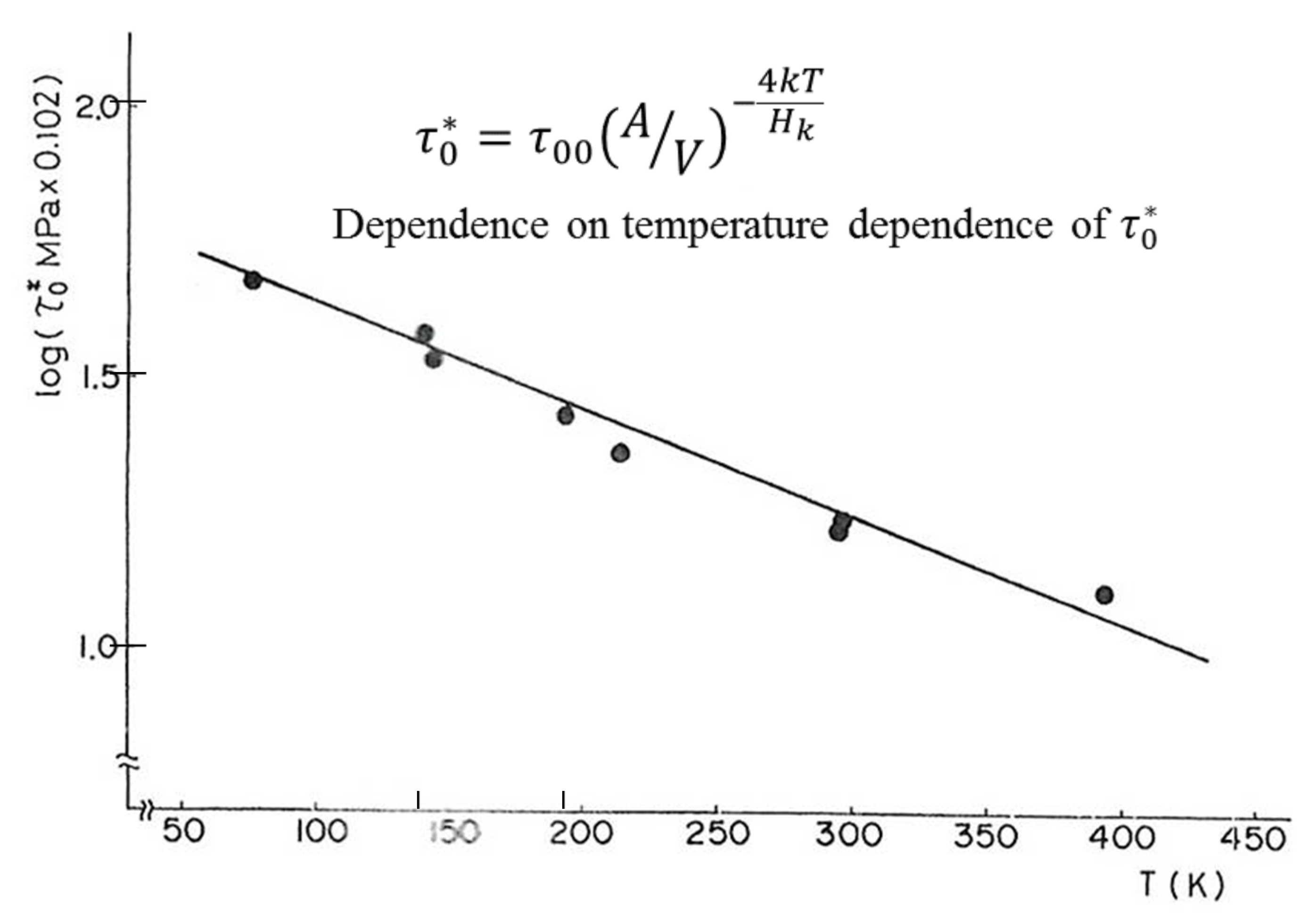
2.5. Application to Problem of Creep

Previous descriptions of the creep rate have been dominated by the use of equations based on the properties of an isolated dislocation [30].

In this section, instead of using the velocity of an isolated equation, the results of dislocation group dynamics associated with emission from a stressed source under constant stress condition were adopted, and a creep rate dominated by the grouped dislocation mechanism was formulated.

The maximum radius of dislocation loop is given by Equations (49) and (50) [30].

$$\mathrm{L}=\sqrt{\frac{2\left({\tau }_a-{\tau }_i\right)}{Gb{\rho }_0^{*}}}$$

(49)

$${\Lambda }^{*}=3\mathrm{L}$$

(50)

By using Equations (27)–(29) and Equation (32), the creep rate, $\acute{\gamma }$, can be given by Equation (51).

$$\acute{\gamma }=A_1{\left({\tau }_a-{\tau }_i\right)}^{\delta }$$

(51)

In (51), ${\tau }_a$ in Equation (32) is replaced by $\left({\tau }_a-{\tau }_i\right)$.

$$\mathsf{\delta }=\frac{2m^2+\frac{9}{2}m+2}{m+2}$$

(52)

$$A_1=3\sqrt{\frac{2{\rho }_0^{*}b}{G}}\times 2.45m^{-0.86}{\left(\frac{Gb}{v_{0}t}\right)}^{-\frac{m+1}{m+2}}\times {\left({\tau }_0^{*}\right)}^{-\frac{m\left(2m+3\right)}{m+2}}{v}_0$$

(53)

Furthermore, when using Equations (7)–(10), the creep rate, $\acute{\gamma }$ is given by Equation (54) as an equation of a thermally-activated process.

$$\acute{\gamma }=C_1{\left({\tau }_a-{\tau }_i\right)}^{{\alpha }_1}exp\left(-\frac{Q_1}{kT}\right)$$

(54)

where

$$C_1=3\sqrt{\frac{2{\rho }_0^{*}b}{G}}\times 2.45m^{-0.86}{A}_1{\left(\frac{Gb}{A_{1}t}\right)}^{-\frac{m+1}{m+2}}\times {\left(G\right)}^{-\frac{m\left(2m+3\right)}{m+2}}$$

(55)

$${\alpha }_1=\frac{2m^2+\frac{9}{2}m+2}{m+2}$$

(56)

$$Q_1=\frac{2m+3}{4\left(m+2\right)}{H}_{k}ln\frac{{\tau }_{00}}{G}$$

(57)

Equation (54) is in good agreement with a pioneering experimental equation given for the creep rate [31]. Since m = 1 is valid for Zn [13], ${\alpha }_1$ is 2.83 in Equation (54), which is in good agreement with experimental data [31]. Thus, Equation (54) is a theoretical equation of a creep rate dominated by a dislocation mechanism that incorporates the effect of dislocation dynamics corresponding to dislocations being emitted from a stressed source.

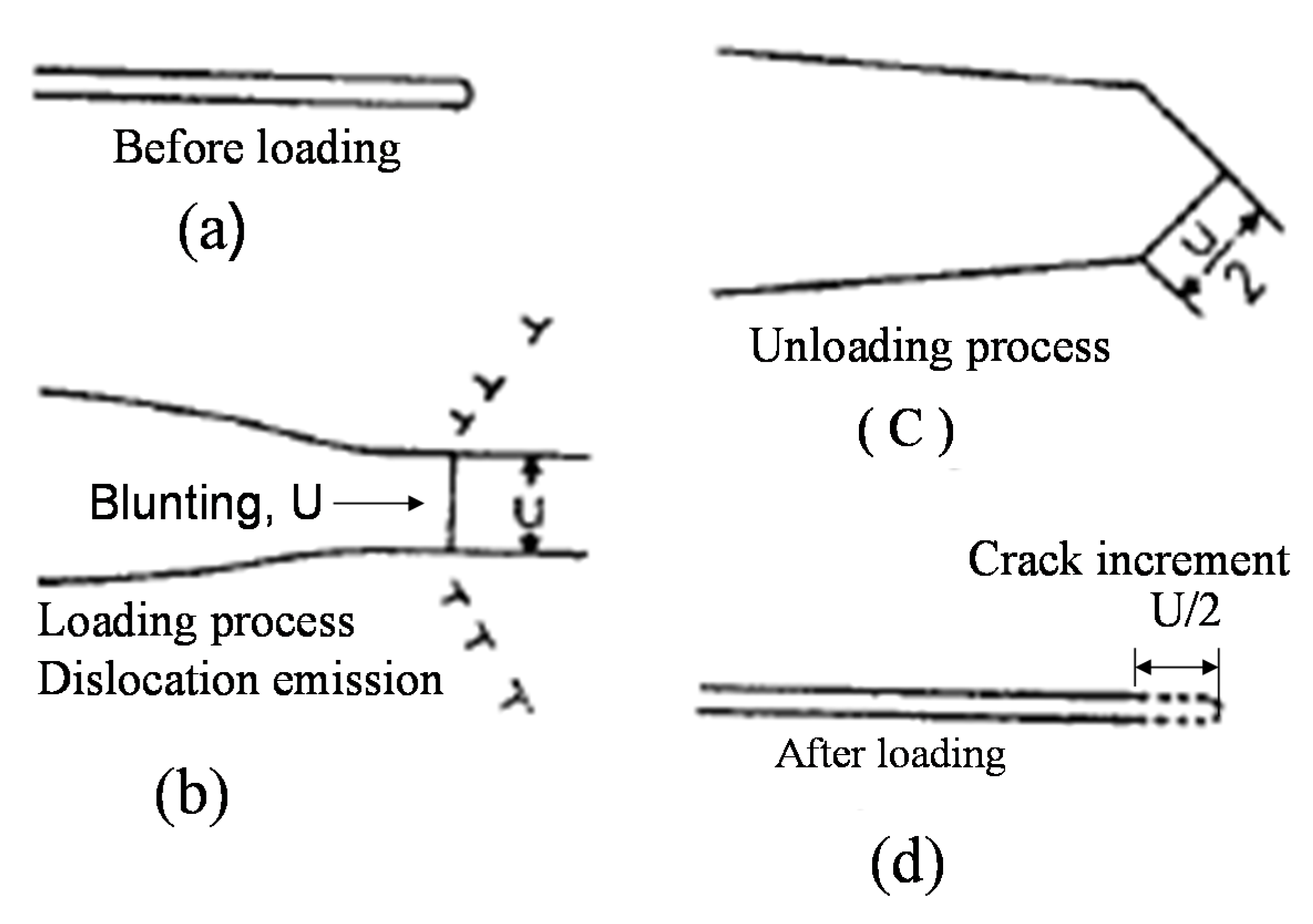
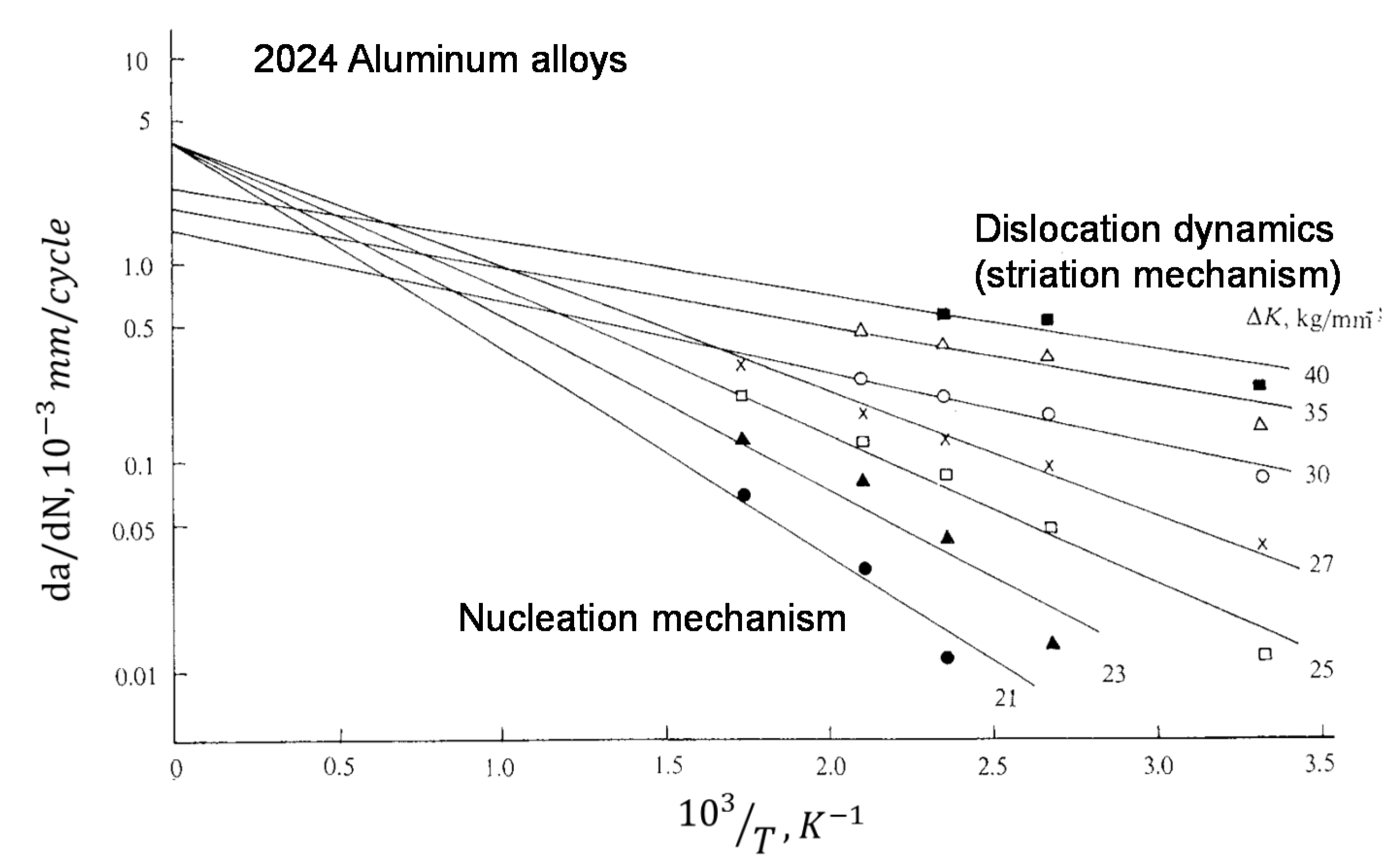
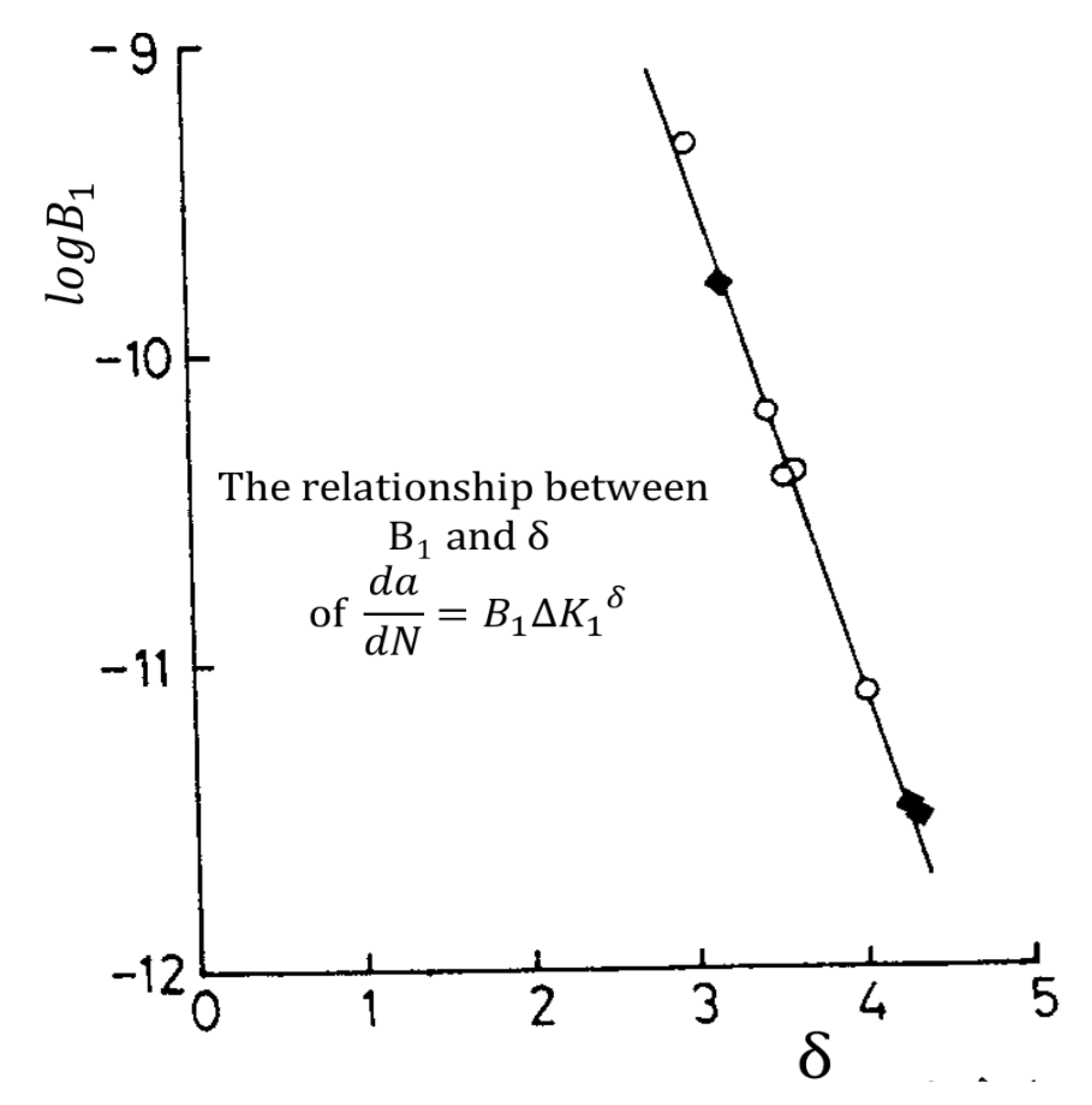
2.6. Application to the Problem of Fatigue Crack Growth [32,33]

The fatigue crack growth rate da/dN for a crack blunting and re-sharpening model [34] is approximately equal to $\frac{1}{2}U$, as shown in Figure 24 [32,33] and given by Equation (58).

$$\frac{da}{dN}\cong \frac{1}{2}U=nb$$

(58)

where U is the crack opening displacement caused by dislocation emission from a crack tip and is equal to 2nb, b is the Burgers vector, and n is the number of dislocations emitted from a crack tip, as shown in Figure 24.

Substituting Equations (6)–(10) into Equation (58) allows for the fatigue crack growth rate to be expressed in terms of an apparent single thermal activated process that is given by Equations (59a) and (59b) [32,33].

$$\frac{da}{dN}=b\gamma \left(m\right){\left(\frac{4fb}{v_0}\right)}^{-\frac{m+1}{m+2}}{\left(\frac{{\tau }_0^{*}}{G}\right)}^{-\frac{m\left(m;1\right)}{m+2}}{\left(\frac{\Delta K_1}{\sqrt{\epsilon }G}\right)}^{\frac{{\left(m+1\right)}^2}{m+2}}$$

(59a)

$$=b{A}^{*}{\left(4f\right)}^{-\frac{m+1}{m+2}}{\left(\frac{\Delta K_1}{\sqrt{\epsilon }G}\right)}^{\frac{m+1}{m+2}}exp\left\{-\frac{\left(\frac{m+1}{m+2}\right)H_{k}ln\left(\frac{{\tau }_{00}\sqrt{\epsilon }}{\Delta K_1}\right)}{4kT}\right\}$$

(59b)

where $\Delta K_1$ is the stress intensity factor, f is load frequency, and $\epsilon$ is the local distance from a crack tip, e.g., $1.5\times {10}^{-4}\mathrm{mm}$. Local stress around a crack tip is characterized given by ${\tau }_a=\frac{\Delta K_1}{\sqrt{\epsilon }}$.

$$A^{*}=1.4m^{-1.45}{\left(\frac{b}{A_1}\right)}^{-\frac{m+1}{m+2}}$$

Equations (59a) and (59b) can be written as Equation (60).

$$ln\frac{da}{dN}=ln\left(\frac{A_2}{f^{\lambda }}\right)+b_{0}ln\Delta K_1-\frac{U_2-a_{2}ln\Delta K_1}{kT}$$

(60)

where $A_2$, $a_2$, and $b_0$ are material constants.

Equations (59a) and (59b) can be expressed as:

$$\frac{da}{dN}=B_1\Delta K_1{}^{\delta }$$

(61)

Which is the well-known experimental Equation by Paris [35], where $\mathsf{\delta }=\frac{{\left(m+1\right)}^2}{\left(m+2\right)}$.

The experimental relationship between $ln\left(\frac{d\mathrm{a}}{\mathrm{dN}}\right)$ and 1/T is shown in Figure 25 [36] with the parameter of stress intensity factor amplitude, $\Delta {\mathrm{K}}_1$.

Figure 25 shows that these relationship were found to hold for the thermally activated process in the range of higher values of $\Delta {\mathrm{K}}_1$, in that the intercept values of the straight line of $ln\left(\frac{d\mathrm{a}}{\mathrm{dN}}\right)$ with the coordinate axis at 1/T = 0 were an approximately linear function of $\ln \left(\Delta {\mathrm{K}}_1\right)$, which is in good agreement with Equation (60), that is, $ln\left(\frac{A_2}{f^{\lambda }}\right)+b_{0}ln\Delta K_1$ [32,33].

On the other hand, in the range of lower values of $\Delta K_1$, the intercept value is constant with stress intensity factor amplitude, $\Delta K_1$, which is in good agreement with the model based on micro crack nucleation at the crack tip [37], given by Equation (62).

$$ln\frac{da}{dN}=ln\left(\frac{A_1}{f}\right)-\frac{U_1-a_{1}ln\Delta K_1}{kT}$$

(62)

where $A_1$ and $a_1$ are material constants. The same experimental tendencies were also found in the relationship between $ln\left(\frac{d\mathrm{a}}{\mathrm{dN}}\right)$ and 1/T for stainless steel [38]. Furthermore, Equation (60) was found to be in good agreement with the experimental relationship between $ln\left(\frac{d\mathrm{a}}{\mathrm{dN}}\right)$ and 1/T for high strength steel at low temperatures [39].

Experimental data showed that da/dN is proportional to $f^{-\lambda }$, and λ experimentally takes values from 0.1 to 0.2 for steel [40] and 0.1 to 0.5 for aluminum alloys [41].

For the case of an elastic–plastic crack, the local stress around a crack tip is written by Equation (63) [42].

$${\sigma }_l=f\left(\beta \right){\sigma }_{cy}{\left(\frac{\Delta K_1}{{\sigma }_{cy}\sqrt{\epsilon }}\right)}^{\frac{2\beta }{1+\beta }}$$

(63)

where ${\sigma }_{cy}$, $\beta$, and $f\left(\beta \right)$ are the initial yield stress in cyclic straining, cyclic strain hardening exponent, and some function of $\mathsf{\beta }$, respectively.

Therefore, by comparing Equations (63), (61), and (59a), da/dN can be given by the following equation [33].

$$\frac{da}{dN}\propto {\left(\frac{\Delta K_1}{\sqrt{2\epsilon }{\sigma }_{cy}}\right)}^{\frac{2\beta }{1+\beta }\frac{{\left(m+1\right)}^2}{m+2}}$$

(64)

Furthermore, for the effect of multiple slip lines and strain hardening under cyclic loading, Equation (64) can be rewritten as Equation (65) [33].

$$\frac{da}{dN}\propto {\left(\frac{\Delta K_1}{\sqrt{2\epsilon }{\sigma }_{cy}}\right)}^{\frac{2\beta }{1+\beta }\frac{{\left(m+1\right)}^2}{m+2}+\frac{1}{1+\beta }}$$

(65)

For β = 0.08–0.3 and m = 4–10, which are reasonable values for steel and aluminum alloys, the power exponent becomes δ = 2.0–5.0, which are also experimentally reasonable values.

In Equation (61), the following equation can be seen from Equation (59a).

$$B_1=B/{\left(\sqrt{\epsilon }G\right)}^{\delta }$$

(66)

From Equation (66), Equation (67) can be obtained [43].

$$ln{B}_1=lnB-\delta ·ln\left(\sqrt{\epsilon }G\right)$$

(67)

Equation (67) was found to be in good agreement with the experimental relationship [43] between $B_1$ and δ, as shown in Figure 26 [43].

3. Concluding Remarks and Future Problem

Analyses of discrete dislocation dynamics and emission from a stressed source were conducted. The results obtained by these analyses enabled us to link various dynamical effects, such as load frequency and temperature, on the yield stress, dislocation creep rate, and fatigue crack growth rate with the experimental results of macroscopic phenomenon and to also link them with theoretical results obtained by the concept of static, continuously distributed infinitesimal dislocations for the equilibrium state under low strain or stress rate conditions.

This will be useful as a holistic research approach relating to the time scale—e.g., ranging from results under high strain rate condition to those under static or low strain rate conditions—and the space scale—e.g., ranging from meso-scale and macro-scale mechanics—that is, from the scale of dislocation groups dynamics to fracture mechanics.

To establish a perfect link of mesoscopic mechanics with macro mechanics and for practical applications to engineering structures, further nonlinear interactive treatments will be necessary, e.g., effects of vacancy diffusion, different multiaxial stress in structures, and different scales of grain boundary influences on dislocation group dynamics. For these study fields, the establishment of inter disciplinary science between material science and structural engineering coupled with computational mechanics is needed as one of future research problems involving the strength of materials.

Detailed research on the effects of grain size and temperature on the yield stress has been systematically conducted, and many innovative results have been obtained [28,29].

The proposed research approach mentioned in this article will enable us to link mesoscopic mechanical factors with macro-scale engineering results [28,29].

Concerning the problems of nano-scale fracturing and plasticity, many studies based on the method of 3D discrete dislocation dynamics have already been successfully conducted [1]. These studies would appear to directly connect with physical properties of dislocations and nano-scale fracturing behaviors. The present results should lead to a wider establishment of fracture prediction in the full range from the nano-scale to macro-scale.

References

1. Zhou, C.; Biner, S.B.; LeSar, R. Discrete dislocation dynamics simulation of plasticity at small scales. Acta Metall. 2010, 58, 1565–1577. [Google Scholar] [CrossRef]
2. Yokobori, T.; Yokobori, A.T., Jr. Physical and Phenomenological Model with Non-Linearity in Ductile fracture and fatigue crack growth. In Physical Non-Linearity’s in Structural Analysis, Proceedings of the IUTAM Symposium, Senlis, France, 27–30 May 1980; Hult, J., Lemaitre, J., Eds.; Springer: Berlin/Heidelberg, Germany, 1980; pp. 271–286. [Google Scholar]
3. Yokobori, A.T., Jr.; Yokobori, T.; Nishi, H. Stress Rate and Grain Size Dependence of Dynamic Stress Intensity Factor by Dynamical Piling-up of Dislocations Emitted. In Proceedings of the IUTAM Symposium on MMMHVDF, Tokyo, Japan, 12–15 August 1985; Kawata, K., Shioiri, J., Eds.; Springer: Berlin/Heidelberg, Germany, 1987; pp. 149–164. [Google Scholar]
4. Suh, N.P.; Lee, R.S. A dislocation model for the delayed yielding phenomenon. Mater. Sci. Eng. 1972, 10, 269–278. [Google Scholar] [CrossRef]
5. Zubelewicz, A. Review Mechanical-based transitional viscoplasticity. Crystals 1972, 10, 212. [Google Scholar] [CrossRef] [Green Version]
6. Yokobori, A.T., Jr.; Yokobori, T.; Kawasaki, T. Computer simulation of dislocation groups dynamics under applied constant stress and its application to yield problems of mild steel. In High Velocity Deformation of Solid; IUTAM Symposium; Kawata, K., Shioiri, J., Eds.; Springer: Berlin/Heidelberg, Germany, 1979; pp. 132–148. [Google Scholar]
7. Cottrell, A.H.; Bilby, B.A. Dislocation theory of yielding and strain ageing of iron. Proc. Phys. Soc. Lond. A 1949, 62, 49–62. [Google Scholar] [CrossRef]
8. Yokobori, T. Delayed yield and strain rate and temperature dependence of yield point in Iron. J. Appl. Phys. 1954, 25, 593–594. [Google Scholar] [CrossRef]
9. Yokobori, T.; Yokobori, A.T., Jr.; Kamei, A. Computer simulation of dislocation emission from a stressed source. Philos. Mag. 1974, 30, 367–378. [Google Scholar] [CrossRef]
10. Yokobori, A.T., Jr.; Yokobori, T.; Kamei, A. Generalization of computer simulation of dislocation emission under constant rate of stress application. J. Appl. Phys. 1975, 46, 3720–3724. [Google Scholar] [CrossRef]
11. Kanninen, M.F.; Rosenfield, A.R. Dynamics of dislocation pile-up formation. Philos. Mag. 1969, 20, 569–587. [Google Scholar] [CrossRef]
12. Rosenfield, A.R.; Hahn, G.T. Linear arrays of moving dislocations emitted by a source. In Dislocation Dynamics; Rosenfield, A.R., Hahn, G.T., Eds.; Mcgraw-Hill: New York, NY, USA, 1968; pp. 255–273. [Google Scholar]
13. Turner, A.P.L.; Vreeland, T. The effect of stress and temperature on the velocity of dislocations in pure iron mono crystals. Acta Metall. 1970, 18, 1225–1235. [Google Scholar] [CrossRef] [Green Version]
14. Seeger, A. On the Theory of the Low-temperature Internal friction Peak Observed in Metals. Philos. Mag. 1956, 1, 651–662. [Google Scholar] [CrossRef]
15. Johnston, W.G. Yield points and delay times in single crystals. J. Appl. Phys. 1962, 33, 2716. [Google Scholar] [CrossRef]
16. Hahn, G.T. A model for yielding with special reference to the yield-point phenomenon of iron and related bcc metals. Acta Metall. 1962, 10, 727–738. [Google Scholar] [CrossRef]
17. Yokobori, T., Jr.; Yokobori, T.; Sakata, H. Derivation of Plastic Strain Rate Formula Based on Dislocation Groups Dynamics and Its Application to Yield Problems. Jpn. Soc. Mech. Eng. 1984, 50, 654–660. (In Japanese) [Google Scholar] [CrossRef]
18. Stein, D.F.; Low, J.R., Jr. Mobility of edge dislocation in silicon-iron crystals. J. Appl. Phys. 1960, 31, 362. [Google Scholar] [CrossRef]
19. Hendrickson, J.A.; Wood, D.S.; Clark, D.S. Prediction of transition in a notched bar impact test. Trans. Am. Soc. Met. 1959, 51, 629. [Google Scholar]
20. Yokobori, T. Zairyo Kyoudogaku, 2nd ed.; Gihodo Pub.: Tokyo, Japan, 1955; Iwanami Pub.: Tokyo, Japan, 1974. [Google Scholar]
21. Gerstle, F.P.; Dvorak, G.J. Dynamics formation and release of a dislocation pile-up against a viscous obstacle. Philos. Mag. 1974, 29, 1337–1346. [Google Scholar] [CrossRef]
22. Sylwestrowicz, W.; Hall, E.O. The deformation and ageing of mild steel. Proc. R. Soc. Lond. B 1951, 64, 405–502. [Google Scholar] [CrossRef]
23. Petch, N.J. The cleavage strength of poly-crystals. J. Iron Steel Inst. 1953, 174, 25–28. [Google Scholar]
24. Armstrong, R.W. The (cleavage) strength of pre-cracked polycrystals. Eng. Fract. Mech. 1987, 28, 529–538. [Google Scholar] [CrossRef]
25. Armstrong, R.W. Material grain size and crack size influences on cleavage fracturing. Philos. Trans. R. Soc. A 2015, 373, 20140124. [Google Scholar] [CrossRef]
26. Cambell, J.D.; Harding, J. Response of Metals to High Velocity Deformation; Inderscience Publishers: New York, NY, USA, 1961; p. 51. [Google Scholar]
27. Manjoine, M.J. Influence of rate of strain and Temperature on yield stress of Mild SteelTrans. J. Appl. Mech. Trans. ASME 1944, 66, A-211. [Google Scholar]
28. Zerilli, F.J.; Armstrong, R.W. Dislocation mechanics based constitutive relations for material dynamics calculations. J. Appl. Phys. 1987, 61, 1816–1825. [Google Scholar] [CrossRef] [Green Version]
29. Armstrong, R.W. Takeo Yokobori and Micro-to Macro-Fracturing of poly-crystals. Strengh Fract. Complex. Int. J. 2020, 12, 79–88. [Google Scholar] [CrossRef]
30. Weertman, J. Steady-state creep through dislocation climb. J. Appl. Phys. 1957, 28, 362. [Google Scholar] [CrossRef]
31. Gilman, J.J. Plastic Anisotropy of Zinc Monocrystals. J. Met. 1956, 8, 1326–1336. [Google Scholar] [CrossRef]
32. Yokobori, T.; Yokobori, A.T., Jr.; Kamei, A. Dislocation dynamics theory for fatigue crack growth. Int. J. Fract. 1975, 11, 781–788. [Google Scholar] [CrossRef]
33. Yokobori, T.; Konosu, S.; Yokobori, A.T., Jr. Micro and Macro Fracture Mechanics Approach to Brittle Fracture and fatigue crack Growth. Fracture 1977, 1, 665–682. [Google Scholar]
34. Laird, C.; Smith, G.C. Crack propagation in high stress fatigue. Philos. Mag. 1962, 7, 847–857. [Google Scholar] [CrossRef]
35. Paris, P. Fatigue: An interdisciplinary approach. In Proceedings of the 10th Sagamore Army Materials Research Conference, Sagamore Conference Center, Raquette Lake, NY, USA, 13–16 August 1963; Burk, J.J., Reed, N.L., Eds.; Syracuse University Press: Syracuse, NY, USA, 1964; p. 107. [Google Scholar]
36. Yokobori, T.; Aizawa, T. The Influence of Temperature and fatigue Crack Propagation rate of Aluminum Alloy. Int. J. Fracture 1973, 9, 489–491. [Google Scholar]
37. Yokobori, T. A Kinetic Approach to Fatigue Crack Propagation. In Physics of Strength and Plasticity; The Orowan Anniversary Volume; Argon, A.S., Ed.; MIT Press: Cambridge, MA, USA, 1969; pp. 327–338. [Google Scholar]
38. Yokobori, T.; Aizawa, T. The influence of temperature and stress intensity factor upon the fatigue crack propagation rate and striation spacing of 304 stainless steel. J. Jpn. Inst. Met. 1975, 39, 1003–1010. (In Japanese) [Google Scholar] [CrossRef] [Green Version]
39. Kawasaki, T.; Nakanishi, S.; Sawaki, Y.; Hatanaka, K.; Yokobori, T. Fracture Toughness and Fatigue Crack Propagation in High Strength Steel at Low Temperature. Jpn. Soc. Mech. Eng. 1975, 41, 3324–3331. (In Japanese) [Google Scholar]
40. Yokobori, T.; Sato, K. The Effect of Frequency on fatigue Crack Propagation Rate and Striation Spacing in 2024-T3 Aluminum Alloy and SM-50 Steel. Eng. Fract. Mech. 1976, 8, 81–88. [Google Scholar]
41. Hartman, A.; Schijve, J. The effect of environment and load frequency on the crack propagation law for macro fatigue crack growth in Aluminum alloys. Eng. Fract. Mech. 1970, 1, 615–631. [Google Scholar] [CrossRef]
42. Rice, J.R. Stress due to a Sharp Notch in a Work-Hardening elastic-Plastic Material Loaded by Longitudinal shear. J. Appl. Mech. 1987, 34, 287–298. [Google Scholar] [CrossRef]
43. Yokobori, T. A Critical evaluation of mathematical equations for fatigue crack growth with special reference to ferritic grain size and monotonic yield strength dependence. In Fatigue Mechanisms; Fong, J., Ed.; ASTMSTP: West Conshohocken, PA, USA; Volume 675, pp. 683–706.
Figure 1. Free expansion model of linear dislocation motion emitted from a stressed source, S.
Metals 10 01048 g001
Figure 2. Discrete dislocation pile-up model with emission from a stressed source.
Metals 10 01048 g002
Figure 3. The stress distribution, τ ( x , t ) , caused by dynamical piling up [3].
Metals 10 01048 g003
Figure 4. The numerical results of stress distribution on the slip line, x > l (S*), near the site of pile-up (barrier) obtained by Equation (15) for the case of N = 14 (Small number of dislocations) [2].
Metals 10 01048 g004
Figure 5. The numerical results of stress distribution on the slip line, x > l (S*), near the site of pile-up (barrier) obtained by Equation (15) for the case of N = 60 (large number of dislocations) [2].
Metals 10 01048 g005
Figure 6. Numerical results of the dynamic stress intensity factor, K d ¯ ( θ ) , due to pile-up by dislocation group dynamics with emission, as well as a comparison with that of a static solution [2].
Metals 10 01048 g006
Figure 7. The values of K d ¯ ( θ ) / K s ¯ ( θ ) plotted against non-dimensional time, θ [2].
Metals 10 01048 g007
Figure 8. The dynamic dislocation density distribution f d for grain size (d) = 0.01; non-dimensional stress rate ( τ ´ τ ´ 0 ) = 10 [3].
Metals 10 01048 g008
Figure 9. The dynamic dislocation density distribution f d for d = 0.005; τ ´ τ ´ 0 = 10 [3].
Metals 10 01048 g009
Figure 10. The dynamic dislocation density distribution f d for d = 0.01; τ ´ τ ´ 0 = 10 5 [3].
Metals 10 01048 g010
Figure 11. The dynamic dislocation density distribution f d for d = 0.05; τ ´ τ ´ 0 = 10 [3].
Metals 10 01048 g011
Figure 12. The relationship between dynamic stress intensity factor controlled by static stress intensity factor and the non-dimensional dynamic factor Θ [3].
Metals 10 01048 g012
Figure 13. The relationship between a non-dimensional constant (A) and d [3].
Metals 10 01048 g013
Figure 14. The relationship between B and τ ˙ τ 0 ˙ [3].
Metals 10 01048 g014
Figure 15. The relationship between dynamic stress intensity factor controlled by static stress intensity and applied stress under constant stress rate condition [3].
Metals 10 01048 g015
Figure 16. The relationship between i = 1 n v i ( t ) v i s o and the number of dislocation emitted from a stressed source, n [17].
Metals 10 01048 g016
Figure 17. The relationship between the delay time of yielding and yield stress based on dislocation dynamics. Solid lines represent the theoretical results [17]. Dotted lines represent the experimental results [19].
Metals 10 01048 g017
Figure 18. The relationship between the delay time of yielding and yield stress based on dislocation dynamics by accounting for the effect of friction stress of dislocation on delay time. Solid lines represent the theoretical results [17]. Dotted lines represent the experimental results [19].
Metals 10 01048 g018
Figure 19. The relationship between upper yield point and constant stress rate based on dislocation dynamics. Solid lines represent the theoretical results [17]. Dotted lines represent experimental results [19].
Metals 10 01048 g019
Figure 20. The relationship between the upper yield point and constant stress rate based on dislocation dynamics by accounting for the effect of friction stress of dislocation on upper yield point. Solid lines represent the theoretical results [17]. Dotted lines represent experimental results [19].
Metals 10 01048 g020
Figure 21. The relationship between τ 0 * , as used for this analysis, and temperature [17].
Metals 10 01048 g021
Figure 22. The relationship between yield strength and grain size, d. Solid line represents the results obtained by the analysis of dislocation dynamic pile, as shown by dotted data [3]. Dotted line represents the solution obtained by Equation (48).
Metals 10 01048 g022
Figure 23. The relationship between strain rate and yield stress of mild steel. Dotted line represents the numerical results [3].
Metals 10 01048 g023
Figure 24. Blunting and re-sharpening model of fatigue crack growth. (a) Before fatigue load cycle, (b) maximum load of the fatigue cycle, (c) unloading process of the fatigue cycle, and (d) complete unloading of the fatigue cycle. The crack increment of U/2 (crack opening displacement/2) is caused by dislocation emission.
Metals 10 01048 g024
Figure 25. The thermally activated relationship between da/dN (fatigue crack growth rate) and the inverse value of absolute temperature, 10 3 T , for 2024 aluminum alloys [36].
Metals 10 01048 g025
Figure 26. The experimental relationship between B1 and δ in Equation (67) [43].
Metals 10 01048 g026