Calculation of Dynamic Coefficients of Air Foil Journal Bearings Using Time-Domain Identification


Abstract
:1. Introduction
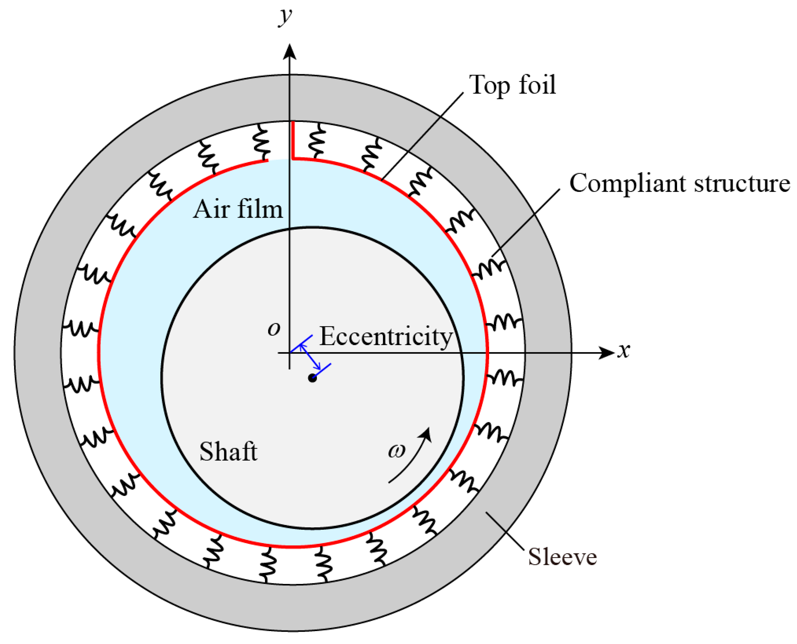
2. Modeling of the Bearing
2.1. Governing Equation
2.1.1. Air Film
2.1.2. Foil Structure
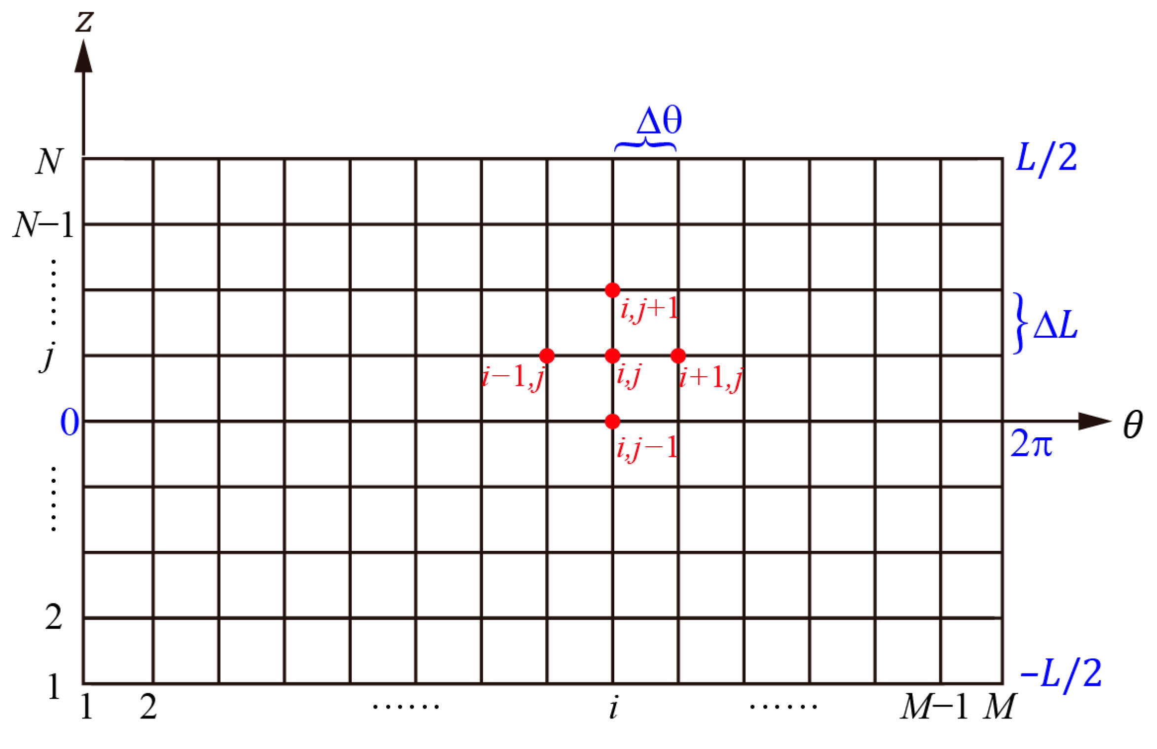
2.2. Discretization and Solution
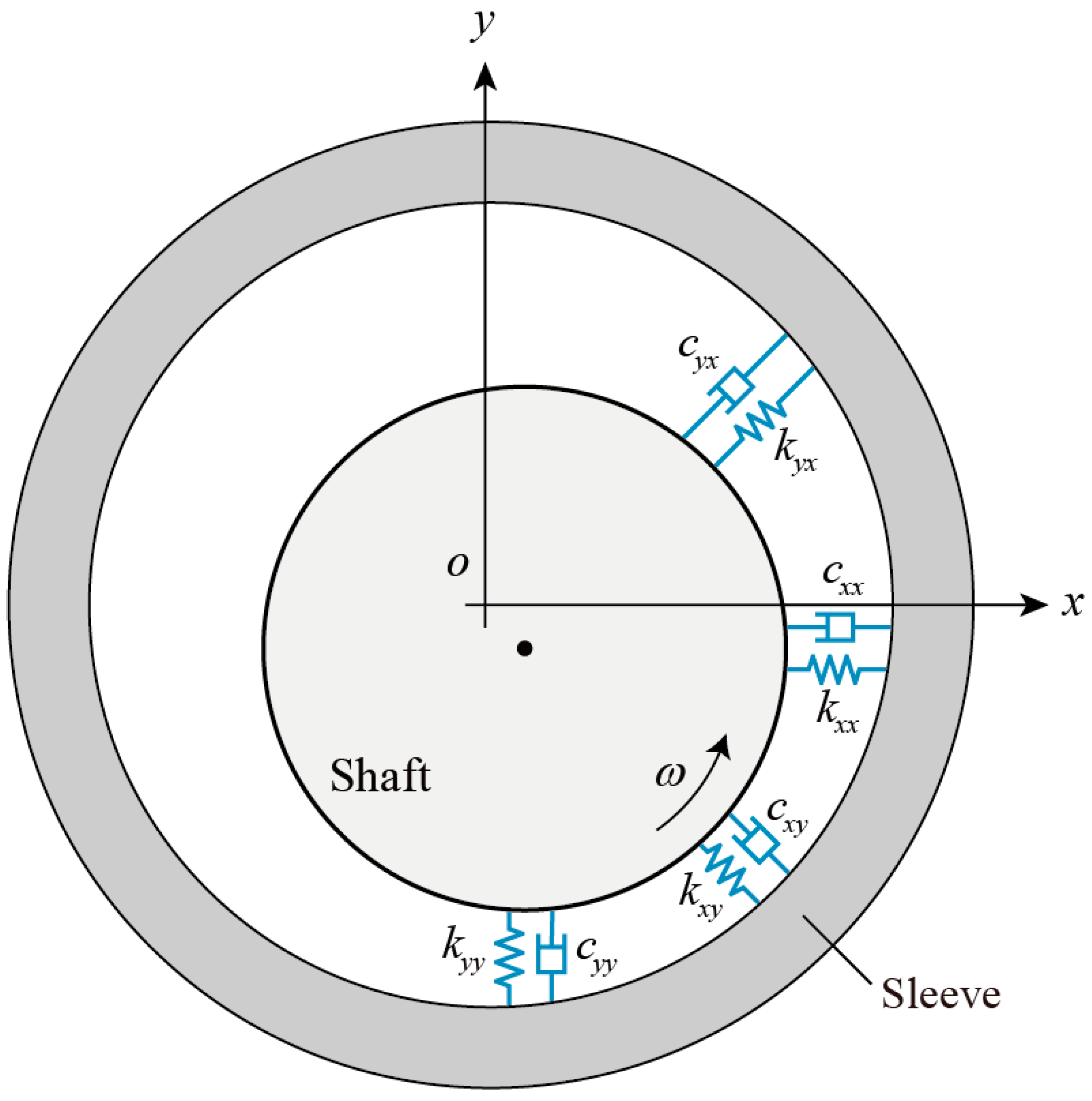
3. Dynamic Coefficients
3.1. Definition
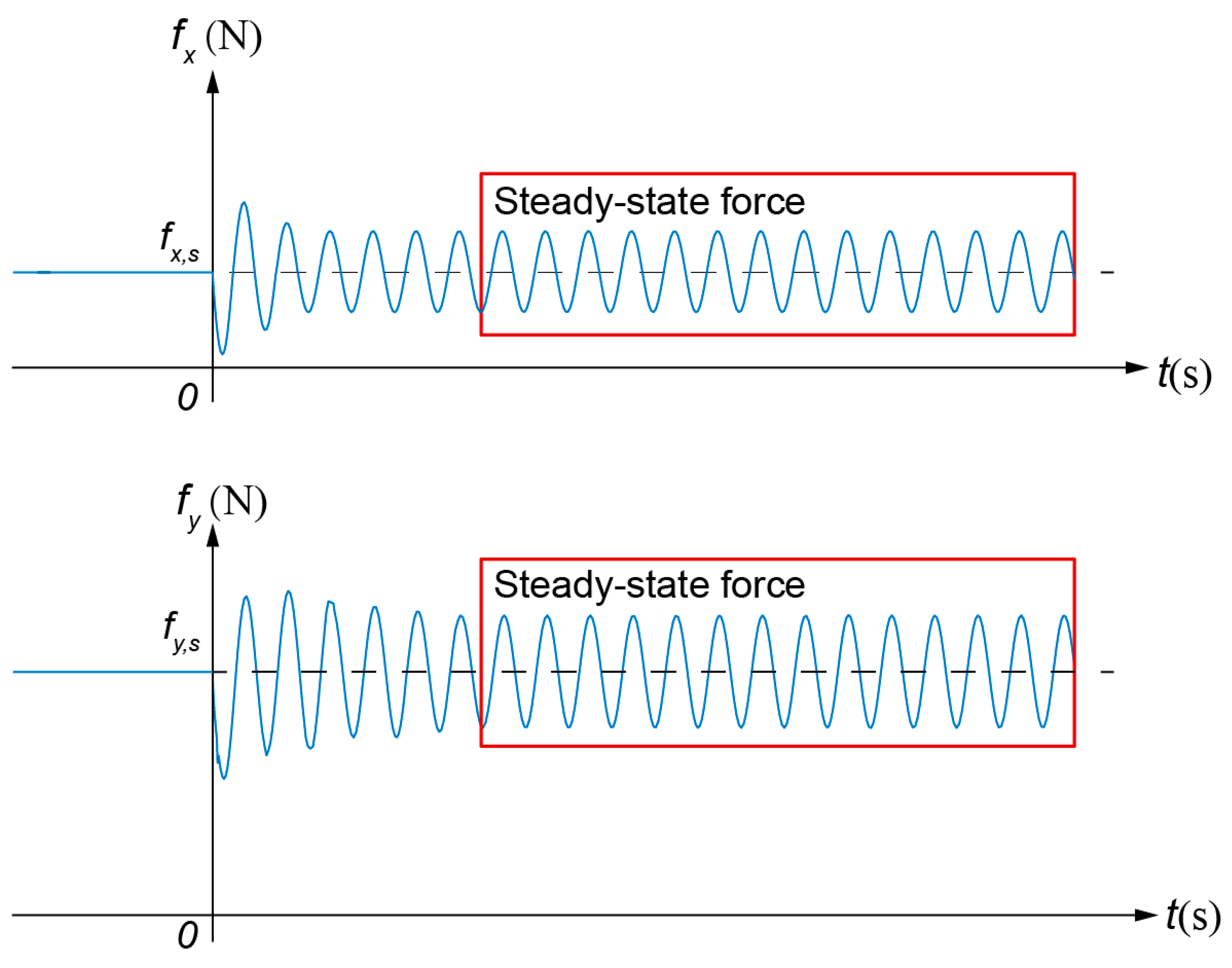
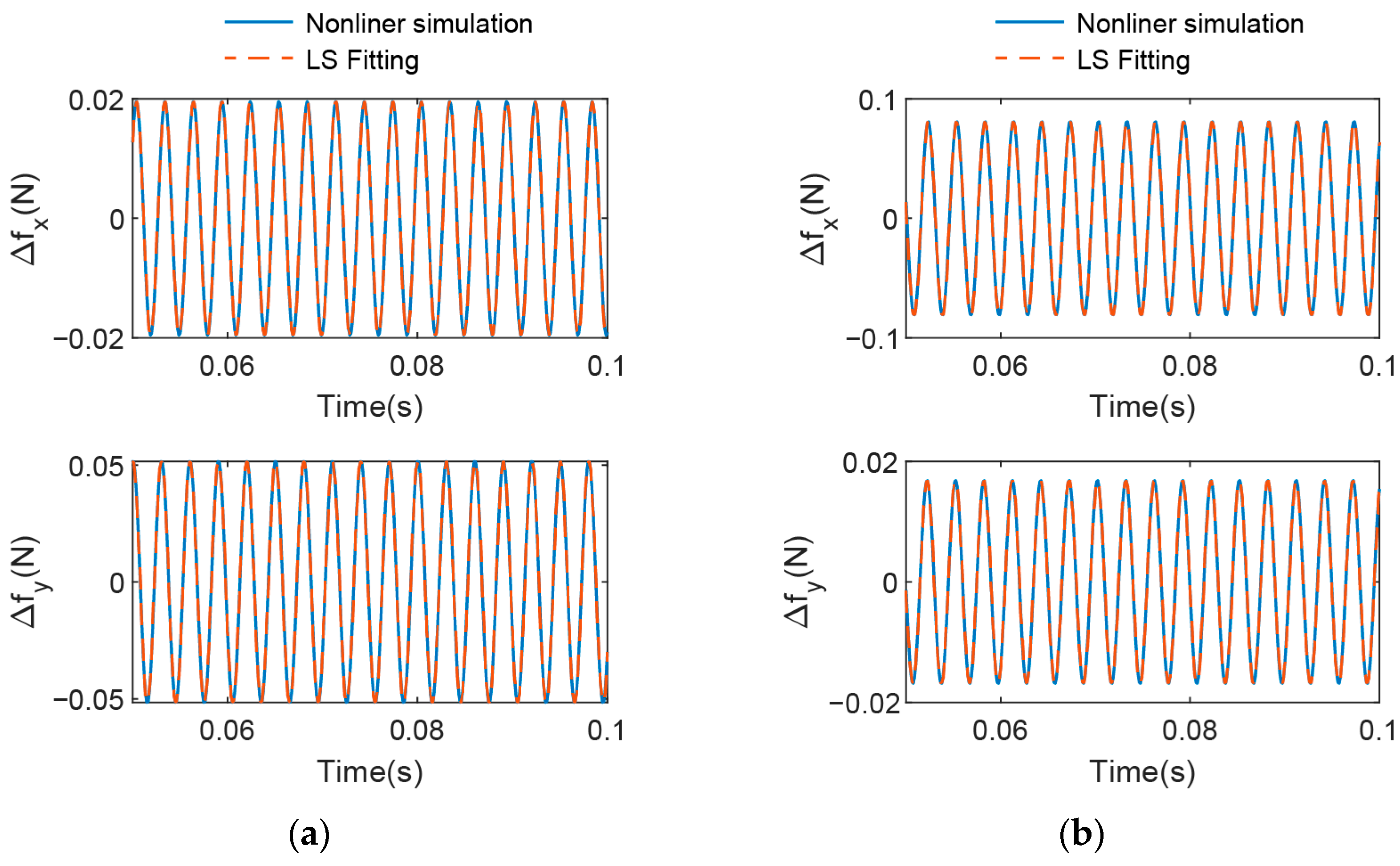
3.2. Calculation
4. Results and Discussion
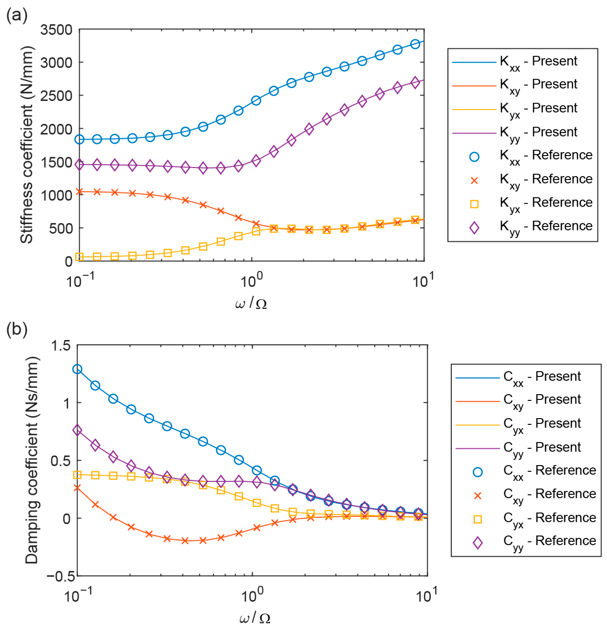
4.1. Verification
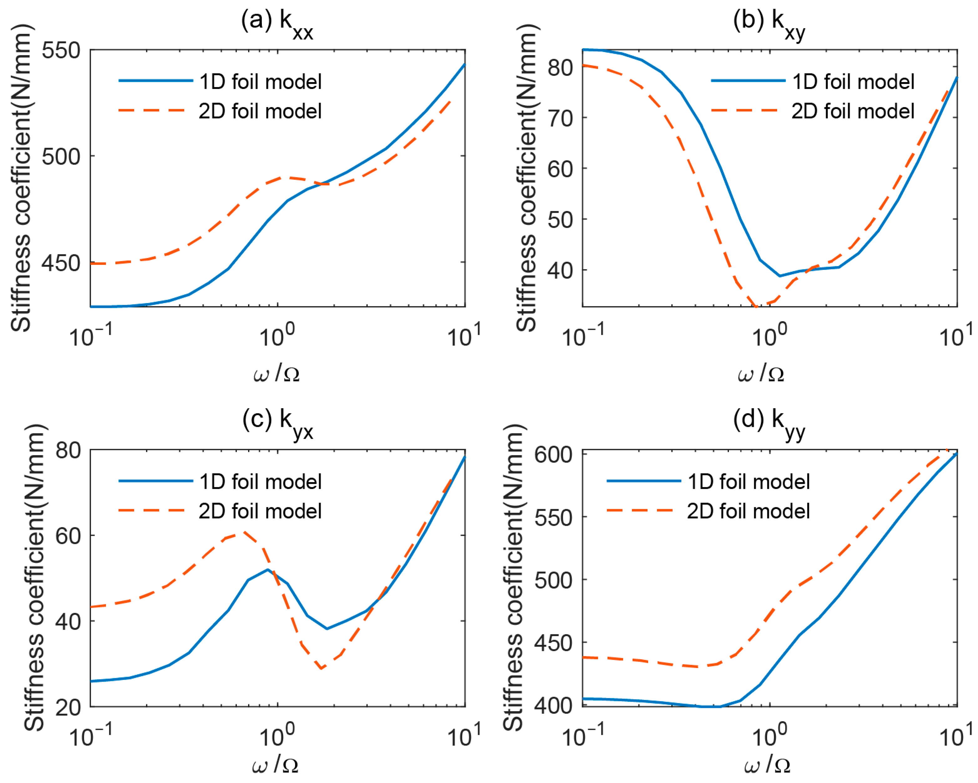
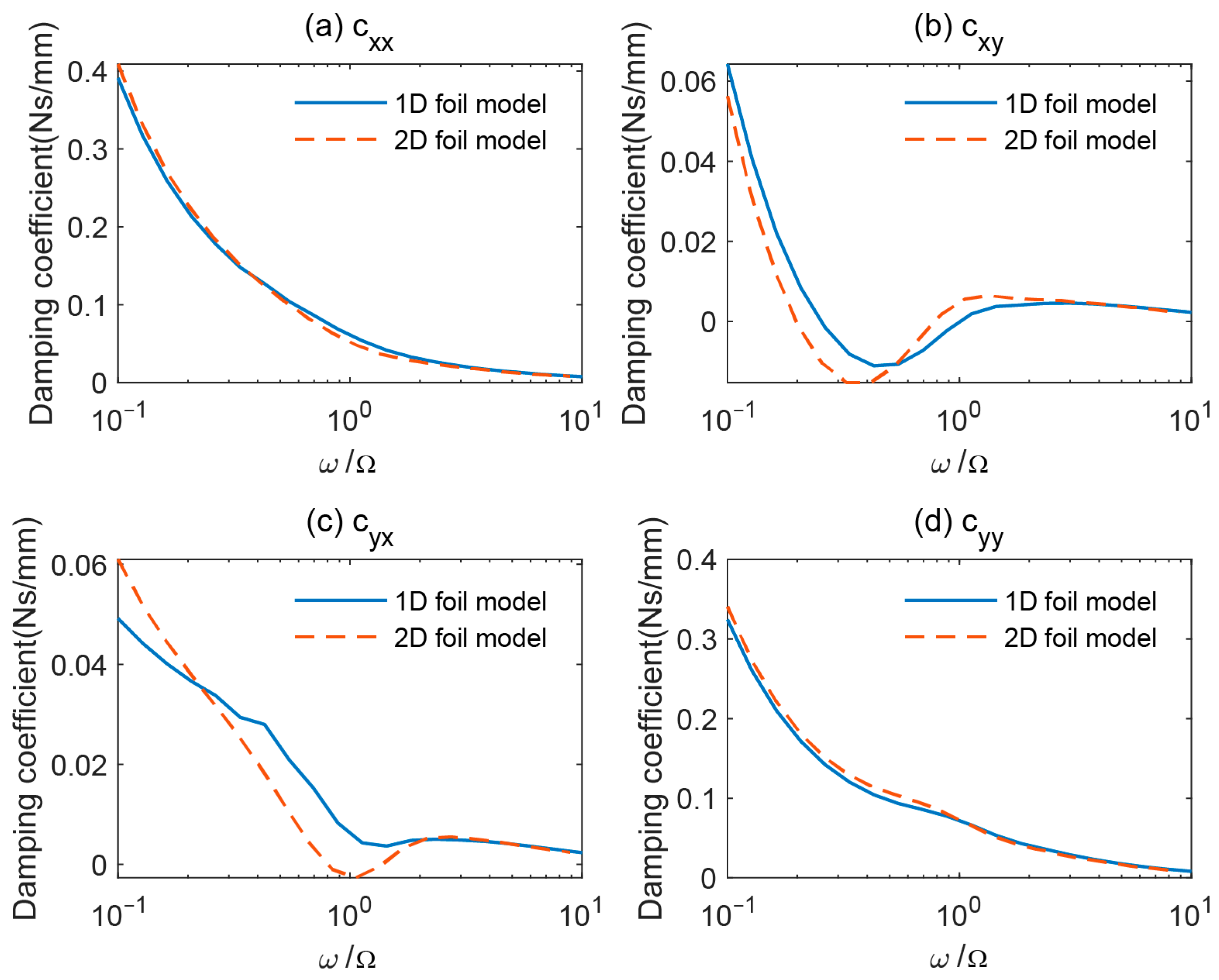
4.2. Comparison of the Results by Two Foil Models
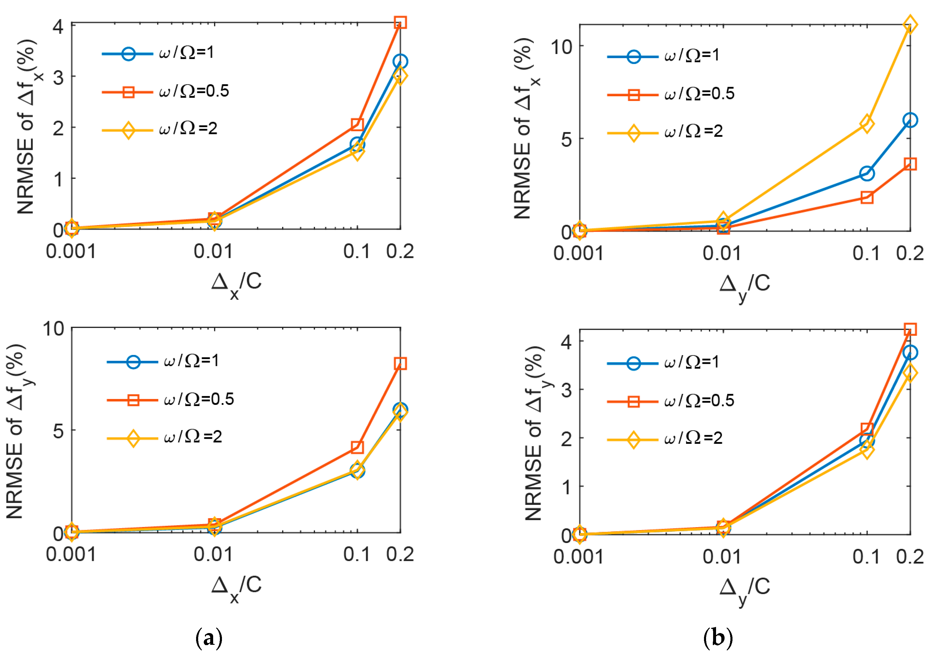
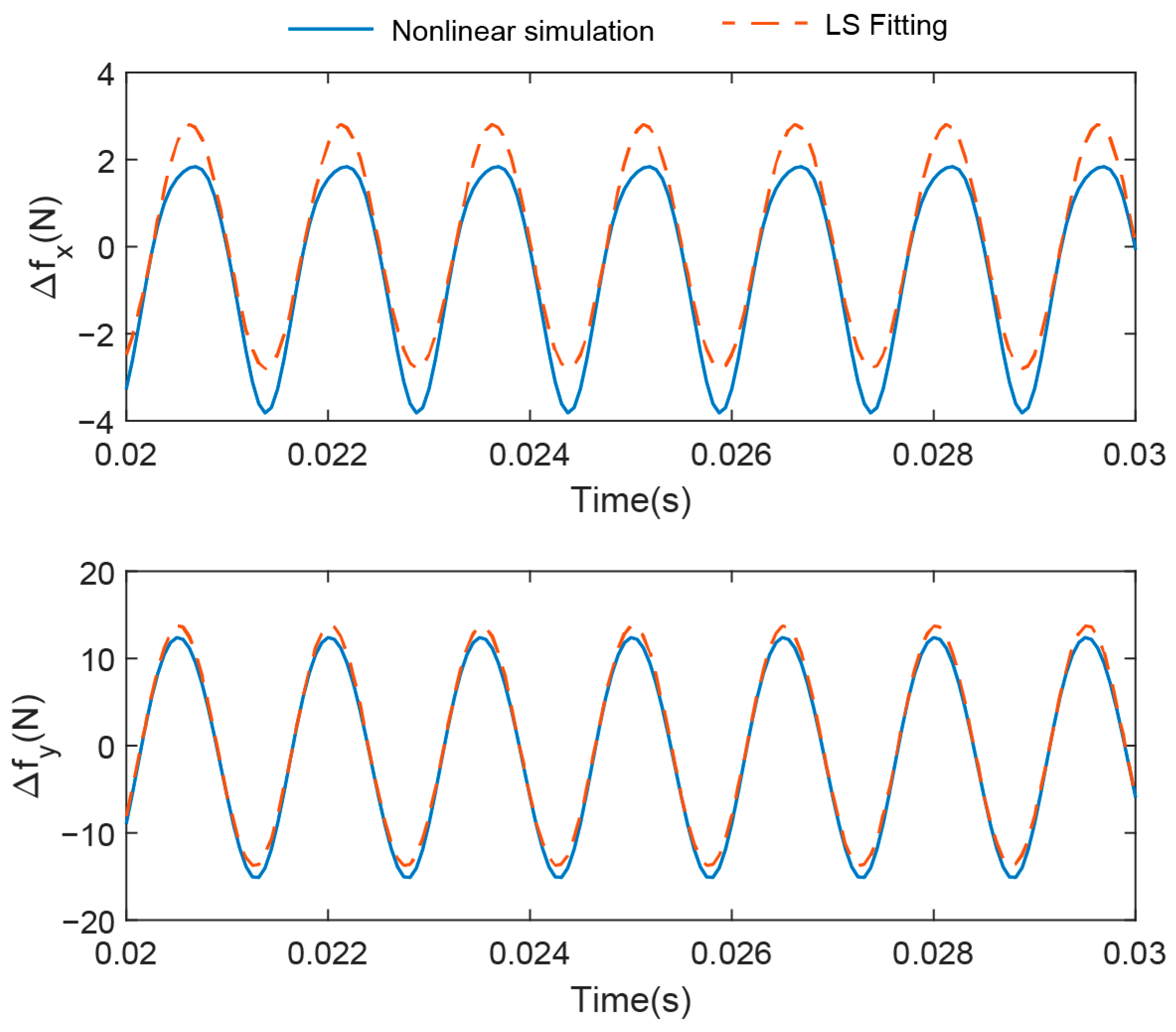
4.3. Influence of the Disturbance Amplitude
5. Conclusions
Author Contributions
Funding
Data Availability Statement
Conflicts of Interest
References
- DellaCorte, C. Oil-Free shaft support system rotordynamics: Past, present and future challenges and opportunities. Mech. Syst. Signal Process. 2012, 29, 67–76. [Google Scholar] [CrossRef] [Green Version]
- Hou, Y.; Zhao, Q.; Guo, Y.; Ren, X.; Lai, T.; Chen, S. Application of Gas Foil Bearings in China. Appl. Sci. 2021, 11, 6210. [Google Scholar] [CrossRef]
- Samanta, P.; Murmu, N.C.; Khonsari, M.M. The evolution of foil bearing technology. Tribol. Int. 2019, 135, 305–323. [Google Scholar] [CrossRef]
- Bou-Saïd, B.; Lahmar, M.; Mouassa, A.; Bouchehit, B. Dynamic Performances of Foil Bearing Supporting a Jeffcot Flexible Rotor System Using FEM. Lubricants 2020, 8, 14. [Google Scholar] [CrossRef] [Green Version]
- Zhou, R.; Gu, Y.; Ren, G.; Yu, S. Modeling and stability characteristics of bump-type gas foil bearing rotor systems considering stick–slip friction. Int. J. Mech. Sci. 2022, 219, 107091. [Google Scholar] [CrossRef]
- Sarrazin, M.; Liebich, R. A Numerical Analysis of the Nonlinear Dynamics of Shimmed Conical Gas Foil Bearings. Appl. Sci. 2023, 13, 5859. [Google Scholar] [CrossRef]
- Lund, J. Spring and damping coefficients for the tilting pad journal bearing. ASLE Trans. 1964, 7, 342–352. [Google Scholar] [CrossRef]
- Lund, J. Calculation of stiffness and damping properties of gas bearings. J. Lubr. Technol. 1968, 90, 793–803. [Google Scholar] [CrossRef]
- Peng, J.; Carpino, M. Calculation of stiffness and damping coefficients for elastically supported gas foil bearings. J. Tribol. 1993, 115, 20–27. [Google Scholar] [CrossRef]
- Lee, Y.B.; Kim, T.H.; Kim, C.H.; Lee, N.S.; Choi, D.H. Unbalance response of a super-critical rotor supported by foil bearings—Comparison with test results. Tribol. Trans. 2004, 47, 54–60. [Google Scholar] [CrossRef]
- Kim, D. Parametric studies on static and dynamic performance of air foil bearings with different top foil geometries and bump stiffness distributions. J. Tribol. 2006, 129, 354–364. [Google Scholar] [CrossRef]
- Vleugels, P.; Waumans, T.; Peirs, J.; Al-Bender, F.; Reynaerts, D. High-speed bearings for micro gas turbines: Stability analysis of foil bearings. J. Micromech. Microeng. 2006, 16, S282. [Google Scholar] [CrossRef]
- Larsen, J.S.; Hansen, A.J.; Santos, I.F. Experimental and theoretical analysis of a rigid rotor supported by air foil bearings. Mech. Ind. 2015, 16, 106. [Google Scholar] [CrossRef] [Green Version]
- Sim, K.; Yong-Bok, L.; Ho Kim, T.; Lee, J. Rotordynamic performance of shimmed gas foil bearings for oil-free turbochargers. J. Tribol. 2012, 134, 031102. [Google Scholar] [CrossRef]
- Han, D.; Bi, C. The Partial Derivative Method for Dynamic Stiffness and Damping Coefficients of Supercritical CO2 Foil Bearings. Lubricants 2022, 10, 307. [Google Scholar] [CrossRef]
- Hoffmann, R.; Munz, O.; Pronobis, T.; Barth, E.; Liebich, R. A valid method of gas foil bearing parameter estimation: A model anchored on experimental data. Proc. Inst. Mech. Eng. C J. Mech. Eng. Sci. 2018, 232, 4510–4527. [Google Scholar] [CrossRef]
- Hoffmann, R.; Pronobis, T.; Liebich, R. Non-linear Stability Analysis of a Modified Gas Foil Bearing Structure. In Proceedings of the 9th IFToMM International Conference on Rotor Dynamics, Milan, Italy, 22 September 2014; Pennacchi, P., Ed.; Springer: Berlin/Heidelberg, Germany, 2015; Volume 21. [Google Scholar] [CrossRef]
- Larsen, J.S.; Santos, I.F.; von Osmanski, S. Stability of rigid rotors supported by air foil bearings: Comparison of two fundamental approaches. J. Sound Vib. 2016, 381, 179–191. [Google Scholar] [CrossRef] [Green Version]
- von Osmanski, S.; Larsen, J.S.; Santos, I.F. Multi-domain stability and modal analysis applied to Gas Foil Bearings: Three approaches. J. Sound Vib. 2021, 472, 115174. [Google Scholar] [CrossRef]
- Gu, Y.; Ren, G.; Zhou, M. A novel method for calculating the dynamic force coefficients of Gas Foil Bearings and its application in the rotordynamic analysis. J. Sound Vib. 2021, 515, 116466. [Google Scholar] [CrossRef]
- Bonello, P.; Pourashraf, T. A comparison of modal analyses of foil-air bearing rotor systems using two alternative linearisation methods. Mech. Syst. Signal Process. 2022, 170, 108714. [Google Scholar] [CrossRef]
- Bonello, P. The extraction of Campbell diagrams from the dynamical system representation of a foil-air bearing rotor model. Mech. Syst. Signal Process. 2019, 129, 502–530. [Google Scholar] [CrossRef]
- Brenkacz, L. Bearing Dynamic Coefficients in Rotordynamics: Computation Methods and Practical Applications; John Wiley & Sons: Hoboken, NJ, USA, 2021. [Google Scholar]
- Bonello, P.; Pham, H.M. The efficient computation of the nonlinear dynamic response of a foil–air bearing rotor system. J. Sound Vib. 2014, 333, 3459–3478. [Google Scholar] [CrossRef]
- Zywica, G.; Baginski, P.; Bogulicz, M.; Martowicz, A.; Roemer, J.; Kantor, S. Numerical identification of the dynamic characteristics of a nonlinear foil bearing structure: Effect of the excitation force amplitude and the assembly preload. J. Sound Vib. 2022, 520, 116663. [Google Scholar] [CrossRef]
- Bonello, P.; Pham, H.M. Nonlinear dynamic analysis of high speed oil-free turbomachinery with focus on stability and self-excited vibration. J. Tribol. 2014, 136, 041705. [Google Scholar] [CrossRef]
- Heshmat, H.; Walowit, J.A.; Pinkus, O. Analysis of gas-lubricated foil journal bearings. J. Lubr. Technol. 1983, 105, 647–655. [Google Scholar] [CrossRef]
- San Andrés, L.; Kim, T.H. Analysis of gas foil bearings integrating FE top foil models. Tribol. Int. 2009, 42, 111–120. [Google Scholar] [CrossRef]
- Gu, Y.; Lan, X.; Ren, G.; Zhou, M. An efficient three-dimensional foil structure model for bump-type gas foil bearings considering friction. Friction 2021, 9, 1450–1463. [Google Scholar] [CrossRef]
- Zhou, R.; Gu, Y.; Cui, J.; Ren, G.; Yu, S. Nonlinear dynamic analysis of supercritical and subcritical Hopf bifurcations in gas foil bearing-rotor systems. Nonlinear Dyn. 2021, 103, 2241–2256. [Google Scholar] [CrossRef]
- Shampine, L.F.; Reichelt, M.W. The MATLAB ODE Suite. SIAM J. Sci. Comput. 1997, 18, 1–35. [Google Scholar] [CrossRef] [Green Version]
- Nielsen, B.; Santos, I.F. Transient and steady state behaviour of elasto–aerodynamic air foil bearings, considering bump foil compliance and top foil inertia and flexibility: A numerical investigation. Proc. Inst. Mech. Eng. Part J J. Eng. Tribol. 2017, 231, 1235–1253. [Google Scholar] [CrossRef]


| Parameter | Value |
|---|---|
| Bearing radius | 19.05 mm |
| Bearing length | 38.1 mm |
| Bearing clearance | 32 μm |
| Foil stiffness | 4.642 N/mm3 |
| Foil hysteretic loss factor | 0.2 |
| Dynamic viscosity | 1.95 × 10⁻⁵ Pa·s |
| Ambient pressure | 101,325 Pa |
| Static load | 30 N |
Disclaimer/Publisher’s Note: The statements, opinions and data contained in all publications are solely those of the individual author(s) and contributor(s) and not of MDPI and/or the editor(s). MDPI and/or the editor(s) disclaim responsibility for any injury to people or property resulting from any ideas, methods, instructions or products referred to in the content. |
© 2023 by the authors. Licensee MDPI, Basel, Switzerland. This article is an open access article distributed under the terms and conditions of the Creative Commons Attribution (CC BY) license (https://creativecommons.org/licenses/by/4.0/).
Share and Cite
Feng, G.; Liu, B.; Li, L.; Zhang, Y. Calculation of Dynamic Coefficients of Air Foil Journal Bearings Using Time-Domain Identification. Lubricants 2023, 11, 294. https://doi.org/10.3390/lubricants11070294
Feng G, Liu B, Li L, Zhang Y. Calculation of Dynamic Coefficients of Air Foil Journal Bearings Using Time-Domain Identification. Lubricants. 2023; 11(7):294. https://doi.org/10.3390/lubricants11070294
Chicago/Turabian StyleFeng, Guangshuo, Bo Liu, Liuyuan Li, and Yiben Zhang. 2023. "Calculation of Dynamic Coefficients of Air Foil Journal Bearings Using Time-Domain Identification" Lubricants 11, no. 7: 294. https://doi.org/10.3390/lubricants11070294