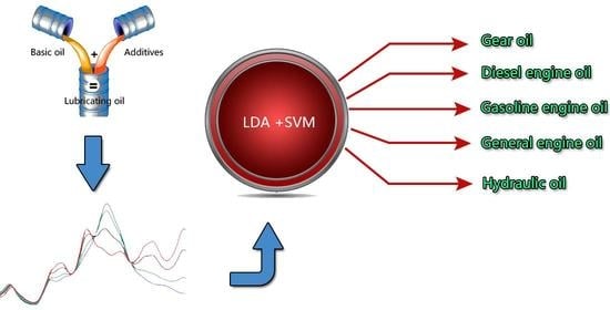
Classification of Lubricating Oil Types Using Mid-Infrared Spectroscopy Combined with Linear Discriminant Analysis–Support Vector Machine Algorithm

Abstract

To realize the classification of lubricating oil types using mid-infrared (MIR) spectroscopy, linear discriminant analysis (LDA) was used for the dimensionality reduction of spectrum data, and the classification model was established based on the support vector machine (SVM). The spectra of the samples were pre-processed by interval selection, Savitzky–Golay smoothing, multiple scattering correction, and normalization. The Kennard–Stone algorithm (K/S) was used to construct the calibration and validation sets. The percentage of correct classification (%CC) was used to evaluate the model. This study compared the results obtained with several chemometric methods: PLS-DA, LDA, principal component analysis (PCA)-SVM, and LDA-SVM in MIR spectroscopy applications. In both calibration and verification sets, the LDA-SVM model achieved 100% favorable results. The PLS-DA analysis performed poorly. The cyclic resistance ratio (CRR) of the calibration set was classified via the LDA and PCA-SVM analysis as 100%, but the CRR of the verification set was not as good. The LDA-SVM model was superior to the other three models; it exhibited good robustness and strong generalization ability, providing a new method for the classification of lubricating oil types by MIR spectroscopy.

1. Introduction

Lubricating oils play a crucial role in industrial practices, serving various functions to ensure the smooth operation of machinery. In the process of mechanical operation, if some parts of the machine do not have the lubrication effect of lubricants, dry friction will occur, causing machine damages. According to experimental data, considerable heat generated by dry friction in a short period of time can melt the metal and even damage the machine. The major working principle is as follows: Lubricating oil which exists between working parts of a machine produces the membrane that can reduce the resistance of the parts in actual work by wrapping an oil film on their surface. Oil films are produced by lubricating oil. Toughness and strength are important indicators for lubricants to play a role. The main aims of gear lubrication are to diminish friction, increase efficiency, reduce wear and contact fatigue of the interacting tooth surfaces, and improve durability [1]. According to the literature [2,3], the gear transmission systems with and without lubrication are very different. A major reduction in energy waste and emissions of mechanical systems can be seen with the optimized performance of lubricating oil [4,5,6].

Lubricating oil mainly comprises basic oil, which governs its basic properties, and additives that enhance the performance of basic oil, providing certain new functions [7]. As seen from data shown in [8,9,10,11,12], lubricants with different types of additives are supposed to lead to different effects.

It is challenging to distinguish the types of lubricating oil solely from their appearance because of the similarities of their constituents: basic oil and small additives. In the process of using lubricating oil, once the label is defaced or lost, it will lead to misuse, which will lead to engine failure, equipment failure, performance gradation, and even accidents. The lubricating oils and the unknown additive types and contents are qualitatively classified and analyzed using physical and chemical methods. Traditional methods, such as Raman spectroscopy [13], physical and chemical characterization, and gas chromatography, are time-consuming and expensive. The composition of lubricating oil is complex, with various types of additives and wide-ranging mid-infrared (MIR) spectroscopy features. Different additives have their own characteristic peaks in the MIR spectra, but because the characteristic peaks seriously overlap, it is challenging to distinguish different lubrication oils directly using MIR, and chemometric methods are required. In recent years, MIR spectroscopy has been widely used in the determination of oil concentration in water [14], molecular structure analysis of new and in-use engine oils [15], analysis of oil sludge [16], determination of soot content in engine oil [17], qualitative and quantitative analysis of sulfur content in crude oil [18], and the detection of oil pollution [19].

Recent research studies on both crude oil and lubricating oil through the method of infrared spectroscopy combined with chemometrics, such as the chemometric strategy based on pattern recognition which has been developed for clustering and the classification of crude oils of Iran, can be seen in the literature [20]. GC-FID and FT-IR fingerprints were considered for fingerprint analysis, and the potential of PCA/HCA for clustering and PLS-DA/CP-ANN for classification were studied. A hybrid optimization method for feature band selection of the middle infrared spectrum based on binary particle swarm optimization (BPSO) and the genetic algorithm (GA) has been developed by Xia Yanqiu et al. [21]. Firstly, the basic classification model of oil additive species recognition by the K nearest neighbor algorithm (KNN) and random forest algorithm (RF) is established. Then, the GA-BPSO hybrid optimization algorithm is used to screen the characteristic band region in the whole band range of the spectrum. O. Galtier et al. [22] compared the results which were obtained by several chemometric methods, SIMCA, PLS2-DA, PLS2-DA with SIMCA, and PLS1-DA, in two infrared spectroscopic applications, which were optimized by selecting spectral ranges containing discriminant information. In the first application, mid-infrared spectra of crude petroleum oils were classified according to their geographical origins. In the second application, near-infrared spectra of French virgin olive oils were classified in five registered designations of origins (RDOs). In both cases, the PLS1-DA classification indicated a 100% good result. An extreme learning machine was used to train and test the model constructed by the infrared spectral data of the mixed additives, and the greedy algorithm and genetic algorithm were used to optimize the input band, while the optimization results were compared. The test results showed both effective identification of the type and prediction of the content of lubricant additives [23]. Owing to the characteristic that the MIR spectroscopy of lubricating oils provides both linear and nonlinear information, the linear discriminant analysis–support vector mechanism (LDA-SVM) model is proposed, which uses LDA for supervised dimensionality reduction, SVM for classification, and provides a theoretical basis for the rapid classification of lubricating oils.

2. Materials and Methods

2.1. Materials

2.1.1. Samples

A total of 120 Lubricating oil samples (Figure 1) from different lubricating oil manufacturers were analyzed using MIR spectroscopy to identify their types: gear oil, n = 13; diesel oil, n = 41; gasoline engine oil, n = 12; general engine oil, n = 33; hydraulic oil, n = 21.

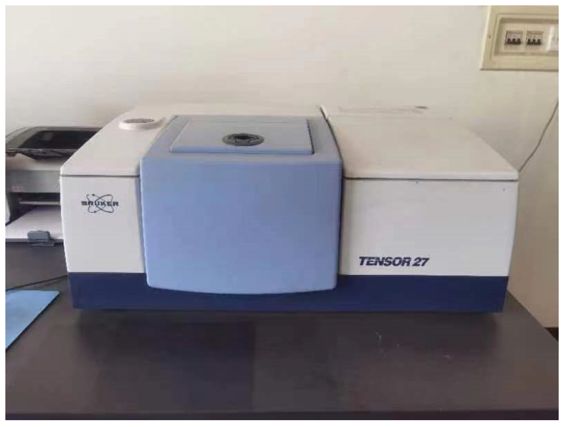
2.1.2. Experimental Instruments and Parameters

Instrument: Tensor27 Fourier transform infrared spectrometer produced by BRUKER (Mannheim, Germany), in Figure 2.

Measurement method: transmission method;

Optical path: 0.1 mm;

Measurement parameters: resolution 4 cm⁻¹;

Beam range: 600–4000 cm⁻¹;

Spectral averaging times: 16 times;

Windows and beam splitters: ZnSe.

Original MIR spectral data of samples are shown in Figure 3.

2.2. Methods

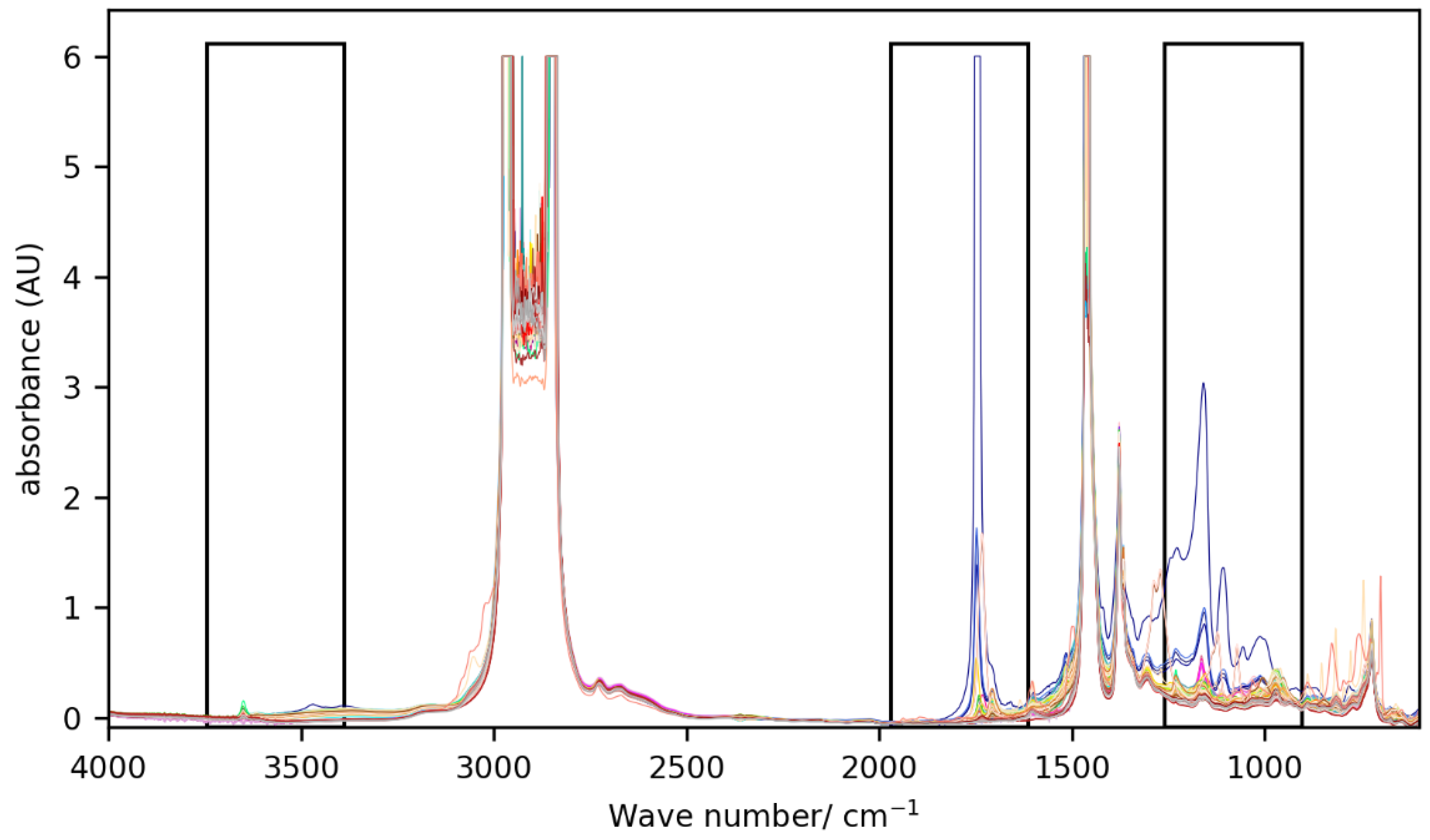
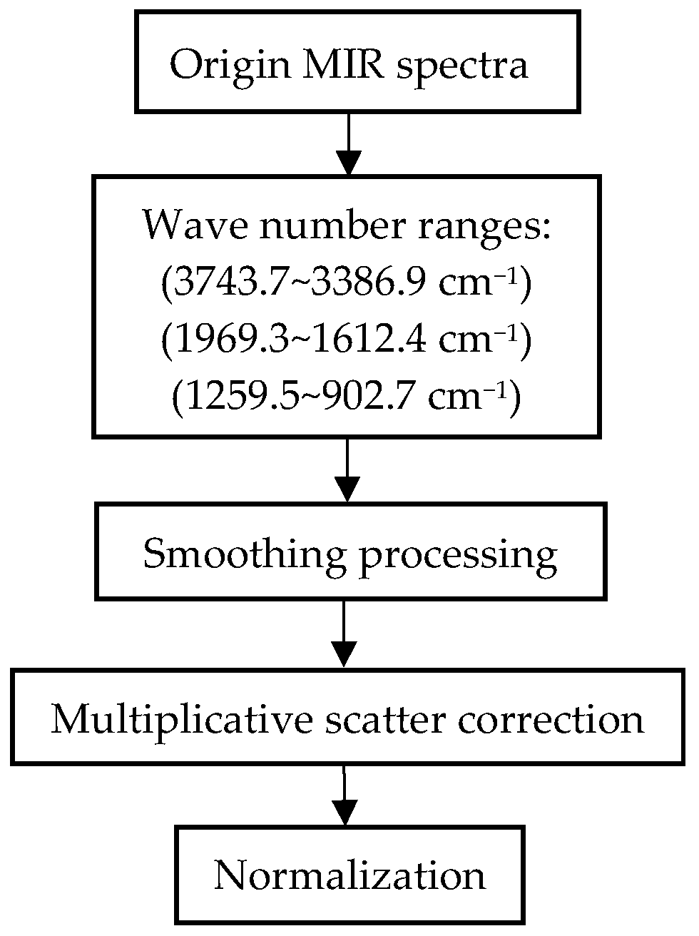
2.2.1. Spectral Data Pre-Processing

Spectral data pre-processing was mainly performed to select the spectral data range and eliminate electrical noise, sample background light, and stray light from the spectral data. The pre-processing method of spectral data greatly influences the stability and generalization ability of the model. In this study, the spectral data pre-processing method was as follows:

(1) Wave number range. Different types of lubricating oils have characteristic peaks in the photon region and fingerprint region of the MIR spectrum, according to the characteristics of the lubrication oil spectrum. The spectral data used in this study consisted of three ranges: 3743.7–3386.9, 1969.3–1612.4, and 1259.5–902.7 cm⁻¹ [7]. Figure 3 shows the MIR spectrum of the original data of the experimental samples. The spectral data in the three black boxes were selected for modeling.

(2) Smooth processing. The Savitzky–Golay convolution smoothing method was used to remove random noise in the spectrum and improve the signal-to-noise ratio.

(3) Multiplicative scatter correction (MSC). MSC was used to eliminate the spectral differences caused by different scattering levels, thereby enhancing the correlation between the spectra and data. Assuming the spectrum $x\left(1\times m\right)$, the MSC algorithm was as follows: ① the average spectrum $\overline{x}$ of the samples was calculated; ② linear regression was performed on $x$ and $\overline{x}$, $x=b_0+\overline{x}b$, and the least squares method was used to determine $b_0$ and $b$; ③ $\left(x-b_0\right)/b_0$.

(4) Normalization. Also known as vector normalization, for a spectrum, first its average absorbance value was calculated, the average value from the spectrum was subtracted, and then the sum of the squares of the spectrum was divided. Normalization can eliminate spectral variations caused by small optical path differences. The normalization calculation formula was as follows:

$$x_k^{\prime }=\frac{x_{ik}-\overline{x}}{\sqrt{{\sum }_{i=1}^n{x}_{ik}^2}}$$

(1)

$\overline{x}$ is mean of the vector, $x_{ik}$ is a value of normalization, $x_k^{\prime }$ is the result of normalization.

Figure 4 shows a flow chart of spectral data pre-processing. The spectral ranges were optimized and selected first and subsequently smoothed; then, MSC and finally normalization were performed.

2.2.2. Dimensionality Reduction Using LDA Algorithm

LDA, proposed by Fisher in 1936, is a supervised dimensionality reduction technology and is widely used in feature extraction. The LDA algorithm predominantly involves projecting the sample data with large dimensions to the best classification vector area to identify the data and narrow the feature range, and after the projection, it ensures that the data have a large inter-class distance and small intra-class distance; that is, the samples can be well separated within this range. Each sample of its dataset has a class output. This is different from principal component analysis (PCA). LDA uses the Fisher discriminant criterion, so it is also known as Fisher’s linear discriminant. The LDA algorithm is widely used in the field of pattern recognition [24,25,26,27,28].

(1) Principle of LDA. Assuming d-dimensional (d features) spectral samples $\mathrm{X}=\left[{\mathrm{X}}_1,\dots ,{\mathrm{X}}_{\mathrm{n}}\right]\in {\mathrm{R}}^{n\times N}$, ${\mathrm{X}}_i\left(i=1,\dots ,N\right)\in {\mathrm{R}}^n$ represents the i-th sample, and N represents the total number of samples. ${\mathrm{X}}_{\mathrm{ij}}\in {\mathrm{R}}^{\mathrm{n}}\left(\mathrm{i}=1,\dots ,c; j=1,\dots ,{\mathrm{N}}_{\mathrm{I}}\right)$ represents the j-th sample in class i, ${\mathrm{N}}_{\mathrm{i}}$ represents the number of samples of the i-th class, and c represents the number of sample classes. The mean of all samples is:

$$\overline{x}=\frac{1}{N}{\sum }_{i=1}^N{x}_i$$

(2)

Let the sample mean of the i-th class be $\overline{x_{\mathrm{i}}}\left(i=1,2,\dots ,c\right)$, then we have

$$\overline{x}={\sum }_{i=1}^c\frac{N_i}{N}{\overline{x}}_i$$

(3)

Dimensionality reduction using LDA is used to reduce high-dimensional spatial feature information to a low-dimensional feature space according to the existing category information. The LDA results show that samples of the same type are clustered together, and samples of different types are separated as much as possible. The inter-class and intra-class distances are expressed in the form of discrete matrices, and the change matrix $W_{opt}$ was solved using Fisher’s criterion. Fisher’s criterion is expressed as follows:

$$J\left(W\right)=\arg max\frac{\left|W^{\mathrm{T}}{S}_{b}W\right|}{\left|W^{\mathrm{T}}{S}_{w}W\right|}$$

(4)

As in (4), $S_b$ is an inter-class discrete matrix, and its specific expression is:

$$S_b={\sum }_{i=1}^c\frac{N_i}{N}\left({\overline{x}}_i-\overline{x}\right){\left({\overline{x}}_i-\overline{x}\right)}^T$$

(5)

As in (4), $S_w$ is an intra-class discrete matrix, and its expression is:

$$S_w={\sum }_{i=1}^c{\sum }_{j=1}^{N_i}\frac{1}{N}\frac{N_i}{N}\left(x_{ij}-\overline{x}\right){\left(x_{ij}-\overline{x}\right)}^T$$

(6)

Equation (4) is the generalized Rayleigh entropy of matrix $S_b$ relative to matrix $S_w$. Using the properties of the generalized Rayleigh entropy, the optimal solution for calculating $J\left(W\right)$ is $W_{opt}=(w_1,w_2,w_3\dots ,w_d)$, where $w_1,w_2,w_3\dots ,w_d$ are the eigenvectors corresponding to the first d non-zero eigenvalues of $S_w^{-1}{S}_b$.

(2) The steps of LDA are as follows:

① Intra-class divergence matrix $S_w$ was calculated;

② Inter-class divergence matrix $S_b$ was calculated;

③ Matrix $S_w^{-1}{S}_b$ was calculated;

④ The largest d eigenvalues of $S_w^{-1}{S}_b$ and the corresponding eigenvectors $\left(w_1, w_{2,}\dots ,w_d\right)$ were calculated to obtain the optimal solution $W_{opt}$;

⑤ $z_i=W_{opt}^T{x}_i$ was calculated for each sample $x_i$ in the sample set;

⑥ The output sample set $D=\left\{\left(z_1,y_1\right),\left(z_2,y_2\right),\dots ,\left(z_m,y_m\right)\right\}$ was obtained.

2.2.3. SVM Algorithm

SVM is a classification technology proposed in 1963 by the AT&T Bell laboratory research group led by Vapnik. SVM is a pattern recognition method based on statistical learning theory, which is mainly used in the field of pattern recognition [29,30]. It provides numerous unique advantages for solving small sample, nonlinear, and high-dimensional pattern recognition, and it can be extended to other machine learning problems such as function fitting. The SVM mechanism involves finding an optimal classification hyperplane that meets the classification requirements so that the hyperplane can maximize the blank areas on both sides of the hyperplane while ensuring classification accuracy. SVM can achieve the optimal classification of linearly separable data.

Taking two types of data classification as examples, given a sample set $\left(x_i,y_i\right), i=1,2,\dots ,l, x\in R^n, y\in \left\{\pm 1\right\}$, with the hyperplane denoted as $\left(w·x\right)+b=0$, to correctly classify all samples and have a classification interval, the following constraints are required:

$$\underset{w,b}{\min }\frac{1}{2}{‖w‖}^2$$

(7)

$$y_i\left[\left(w·x_i\right)+b\right]\ge 1; i=1,2,3\dots l$$

(8)

This is a convex quadratic programming problem that was solved using the Lagrange function:

$$\mathrm{L}\left(w,b,a\right)=\frac{1}{2}‖w‖-a\left(y\left(\left(w·x\right)+b\right)-1\right)$$

(9)

The optimal solution was determined by finding the maximum value:

$${\mathit{a}}^{*}={\left(a_1^{*},a_2^{*},a_3^{*},\dots ,a_l^{*}\right)}^{\mathrm{T}}$$

(10)

The optimal weight vector $w^{*}$ and the optimal bias $b^{*}$ were calculated as follows:

$$w^{*}={\sum }_{j=1}^l{a}_j^{*}{y}_j{x}_j$$

(11)

$$b^{*}=y_i-{\sum }_{j=1}^l{y}_j{a}_j^{*}\left(x_j·x_i\right)$$

(12)

For the linear inseparable case, the kernel method was used. The main idea was to project the input vector to a high-dimensional feature vector space and construct the optimal classification surface in the feature space. The linear discriminant function was constructed in the high-dimensional space, and the commonly used kernel functions were as follows:

① Linear kernel function: $K\left(x,x_i\right)=〈x,x_i〉$;

② Polynomial kernel function: $K\left(x,x_i\right)={\left[\gamma \left(x·x_i\right)+coef\right]}^d$, where d is the order of the polynomial, and coef is the bias coefficient;

③ RBF kernel function: $K\left(x,x_i\right)=\exp \left(-\gamma {‖x-x_i‖}^2\right)$, where $\gamma$ is the width of the kernel function;

④ Sigmoid kernel function: $K\left(x,x_i\right)=\tanh \left(\gamma \left(x·x_i\right)+coef\right)$, where γ is the width of the kernel function and coef is the bias coefficient.

2.3. Construction of Calibration Set and Validation Set

2.3.1. K/S Algorithm

The K/S algorithm [31] can provide the best expression of the difference between samples and select more representative samples. The K/S algorithm was used to select the sample set, and the steps were as follows: (1) The Euclidean distance between the two samples was calculated, and the two samples with the largest distance were selected for the calibration set. (2) The distance between each remaining sample and the selected calibration set was calculated, and the two farthest and nearest samples were determined and selected for the calibration set. (3) Step (2) was repeated until the number of the selected calibration samples was equal to the predetermined number. (4) The remaining samples were the samples of the validation set.

2.3.2. Specific Construction of Calibration Set and Validation Set

The calibration set and verification set were constructed by the K/S algorithm with a ratio of 6:4 for the spectral data of gear oil, diesel oil, gasoline oil, general oil, and hydraulic oil samples. The specific sample distribution is listed in

Table 1. Composition of calibration and validation set.

Sample Types	Calibration Set	Validation Set	Sum of Sample
Gear oil	8	5	13
Diesel engine oil	25	16	41
Gasoline engine oil	8	5	13
All-purpose engine oil	20	13	33
Hydraulic oil	13	9	22
Total number of samples	74	46	120

, and the statistical distribution of MIR spectral data of samples in the calibration set and prediction set is listed in

Table 2. Statistical distribution of MIR spectral data of samples in calibration set and prediction set.

Sample (Unit)	Data Sets	Number of Samples	Maximum	Minimum	Mean	Standard Deviation
Lubricating oils	Calibration set	74	6.0	−0.065	0.070	0.163
	Validation set	46	1.732	−0.063	0.064	0.117

.

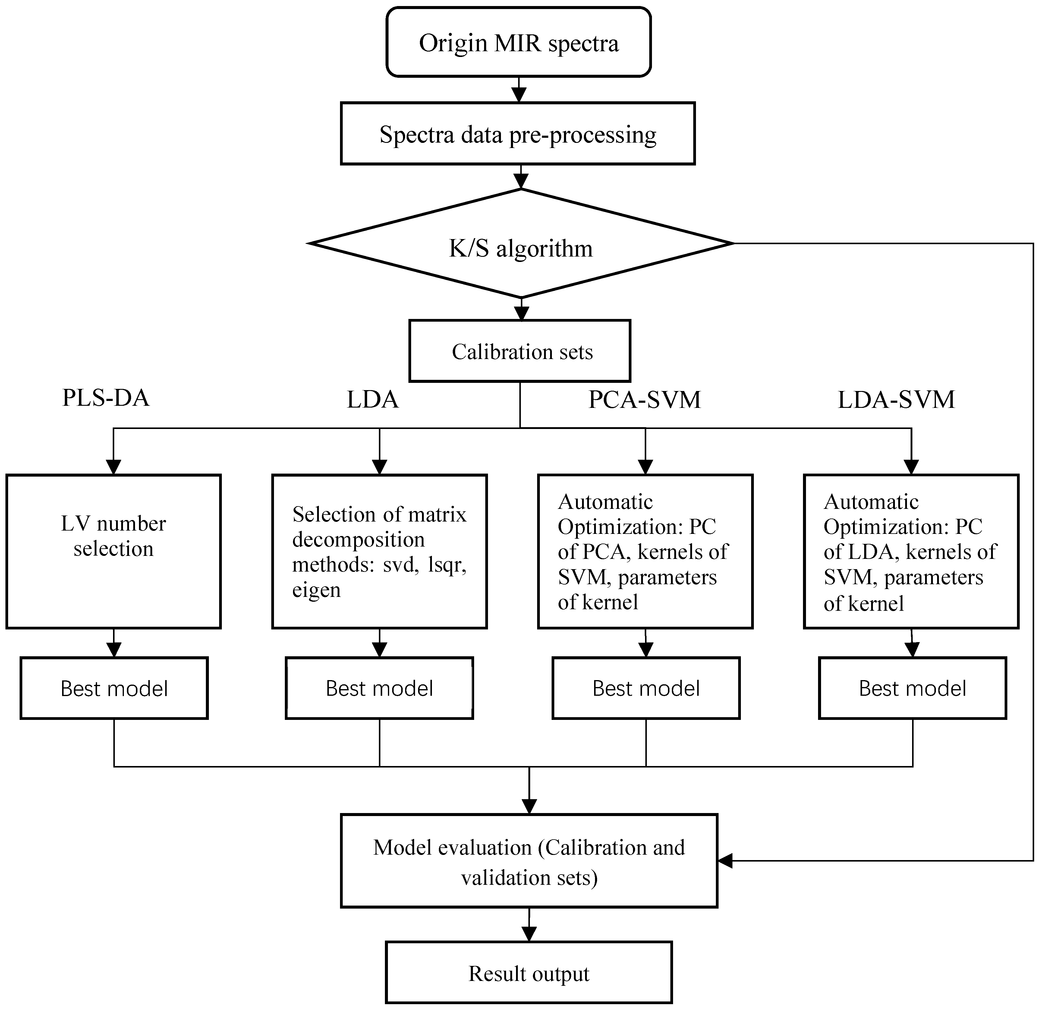
2.4. LDA-SVM Algorithm Steps

Step 1: Data pre-processing. The spectral range was optimized, the signal-to-noise ratio was improved, and the influence of stray light was eliminated;

Step 2: The K/S algorithm was used to divide the sample data to ensure the representativeness of the calibration set and validation set;

Step 3: Supervised dimensionality reduction was performed on the calibration set using LDA, and the optimal vector $W_{opt}$ was calculated;

Step 4: The dimensionality reduction result was provided as the input of SVM, and the grid search method was used to automatically search and calculate the optimal parameters of SVM, when the kernel functions were linear, poly, RBF, and sigmoid;

Step 5: The dimensionality reduction result of the validation set was calculated through the optimal vector $W_{opt}$ obtained in step 3;

Step 6: The optimal parameters were used to predict the validation set through SVM.

2.5. Experimental Design

As shown in Figure 5, the original infrared spectrum data of the lubricating oils were pre-processed, the data were divided into calibration and validation sets by the K/S algorithm, and the calibration set was input into four models: 1. The PLS-DA model was used to calculate the percentage of correct classification (%CC) of the calibration set under different latent variable numbers, and the principal component number with the highest correct rate was selected. 2. The LDA model, when the matrix was decomposed with singular value decomposition (SVD), least square (lsqr), eigenvalue decomposition (eigen), and the %CC of the calibration set and validation set were calculated, and the optimal results were selected. 3. When the principal component number of PCA was 2–40, the results of dimensionality reduction were used as the input of SVM. The grid search method was used to search the hyperparameters automatically to obtain the optimal solutions of the kernel functions when they were linear, poly, RBF, and sigmoid. 4. The principal component number of LDA was 2, 3, or 4, the dimension reduction results were taken as the input of SVM, and the grid search method was used to search the hyperparameters automatically to obtain the optimal solutions of kernel functions when they were linear, poly, RBF, and sigmoid.

The %CC was the criterion used to compare classification results.

%CC = N_c/(N_c + N_ic)

(13)

where N_c and N_ic represent the numbers of incorrect and correct identifiers, respectively.

PLS-DA, LDA, PCA-SVM, and LDA-SVM models were built using the Keras and Scikit-learn machine learning library. They were developed based on Python 3.7.0, and the data mining and data analysis tools adopted Scikit-learn 0.23.2. The programming platform is based on Jupiter Notebook 4.4.0 and runs on the Windows 10 operating system.

3. Results and Discussion

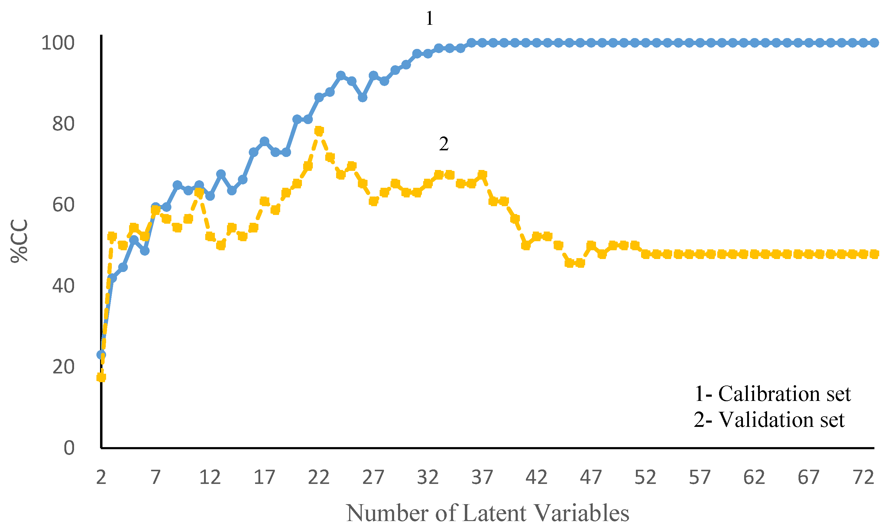
3.1. PLS-DA Model

The number of latent variables is an important parameter in the PLS-DA model; when the number of latent variables is small, it leads to insufficient feature extraction, and when the number of latent variables is large, it leads to noise information. The %CC of the calibration and validation sets is shown in Figure 6. The number of latent variables ranges from 2 to 74, and the %CC of the calibration set increases with the number of latent variables; when the number of latent variables is >36, the cyclic resistance ratio (CRR) remains unchanged at 100%. The %CC of the validation set fluctuated greatly with the number of latent variables, and when the number of latent variables was 22, the %CC reached its maximum, 78%. The PLS-DA model was over-fitted by comparing the results of calibration and validation sets. When the number of latent variables was 22, the sum of the %CC of the calibration and validation sets reached the maximum value.

3.2. LDA Model

The %CC of the calibration and validation sets is listed in

Table 3. %CC for calibration and validation sets under different decomposition methods with LDA model.

Decomposition Method	Calibration Sets (%CC)	Validation Sets (%CC)
SVD	100	95
sqlr	95	97
eigen	95	97

; different matrix decomposition algorithms have a certain influence on the results of the LDA model. When the matrix decomposition algorithms were used by SVD, the %CC of the calibration and validation sets was 100% and 95%, respectively. When the matrix decomposition algorithms were used by lsqr and eigen, the %CC of the calibration and validation sets was 95% and 98%, respectively. By comparing the three decomposition algorithms, we observe that SVD decomposition algorithms are favorable, where the sum of the %CC of the calibration and validation sets reaches the highest value.

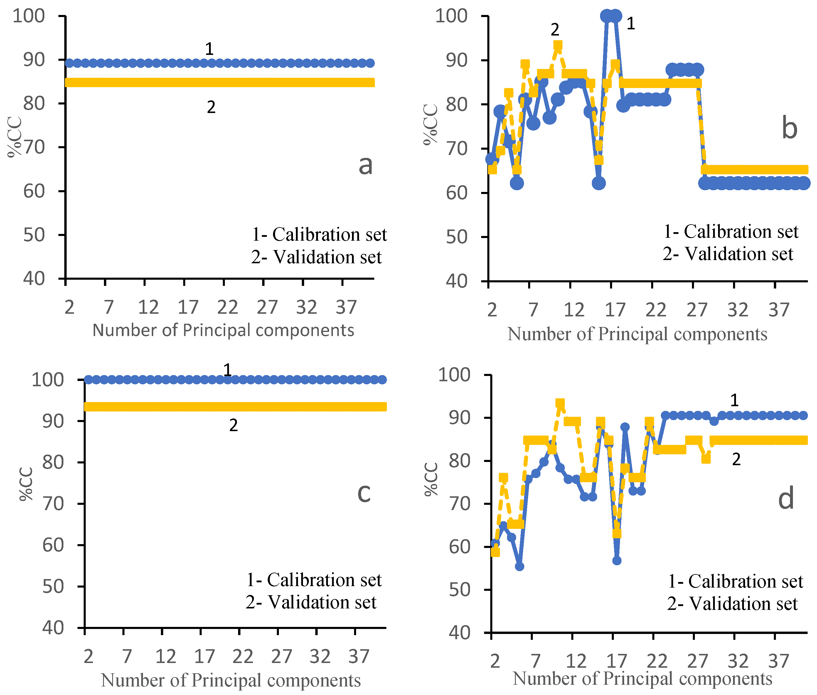
3.3. PCA-SVM Model Recognition Results

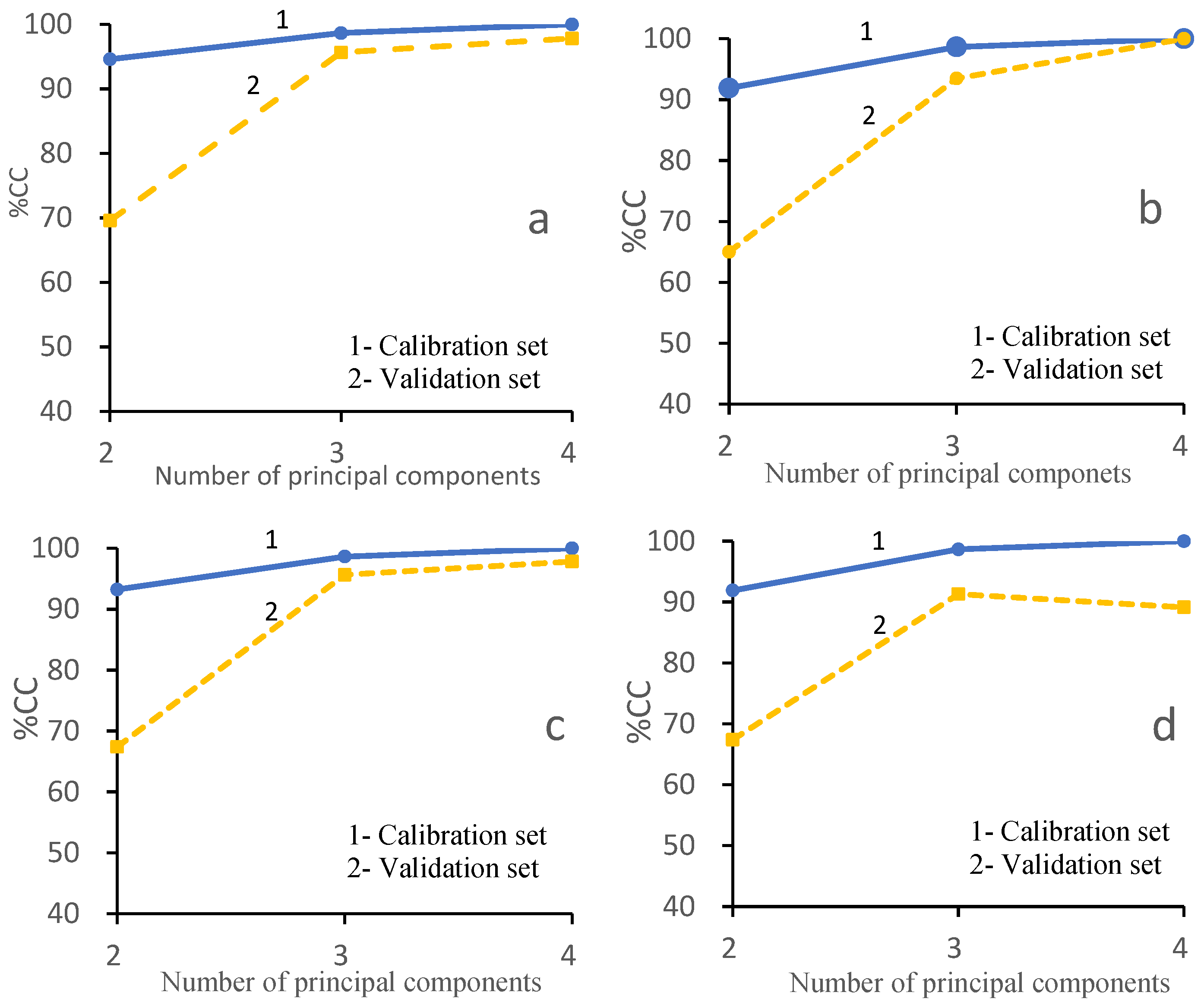
PCA is an unsupervised dimensionality reduction technique. The main factors affecting the PCA-SVM model are as follows: principal component number, kernel function, and kernel function parameters. The kernel functions of SVM are linear, poly, RBF, and sigmoid when the principal component number ranges from 2 to 42, and grid search is used for automatic hyperparameter search. As shown in Figure 7a,c, the principal component numbers negligibly influence the linear and RBF kernel functions. When the kernel functions are linear, the %CC of the calibration and validation sets are 89% and 85%, respectively, When the kernel functions are RBF, the %CC of the calibration and validation sets is 100% and 93%, respectively. As shown in Figure 7b, when the kernel function is poly, the %CC of the calibration and validation sets increases first and then decreases. When the principal component number is 16, the %CC of the calibration and validation sets is 100% and 89%, respectively. As shown in Figure 7d, the %CC of the calibration and validation sets increases with an increase in the principal component number and finally stabilizes. When the principal component number is 30, the %CC of calibration and validation sets is 91% and 89%, respectively. Comparing the results of the different kernel functions, the best prediction result of the PCA-SVM model is achieved using the RBF kernel function, and the %CC of the calibration and validation sets is 100% and 93%, respectively.

3.4. LDA-SVM Model

LDA is a dimensionality reduction technique. The main factors that affect the classification results of the LDA-SVM model are as follows: the principal component number, kernel function, and kernel function parameters. When the principal component number is 2, 3, or 4, and the kernel functions of SVM are linear, poly, RBF, and sigmoid, respectively, grid search is used for automatic hyperparameter search to obtain the optimal solutions. The %CC of the calibration and validation sets is listed in Figure 8. The %CC of the calibration and validation sets increases with an increase in the principal component number of LDA, and when the principal component number is 4, the %CC of the calibration and validation sets becomes maximized. Comparing the results of different kernel functions, the best prediction result of the PCA-SVM model is exhibited by the poly kernel function, and the %CC of the calibration and validation sets is 100%.

3.5. Comparison of Model Classification Results

The classification results of PLS-DA, LDA, PCA-SVM, and LDA-SVM are listed in

Table 4. Correct classification of calibration and validation sets of different models.

Model	Parameter	Calibration Sets (%CC)	Validation Sets (%CC)
PLS-DA	LV = 22	86%	78%
LDA	Decomposition method = SVD	100%	95%
PCA-SVM	PC = 2, kernel = RBF	100%	94%
LDA-SVM	PC = 4, kernel = poly	100%	100%

. The PLS-DA model exhibits the worst recognition ability, the over-fitting phenomenon is serious, and the CRR of calibration and validation sets is poor. When classified using the LDA and PCA-SVM model, the CRR of the calibration set achieved 100%, but the CRR of the validation set is unfavorable; the LDA-SVM has the best recognition, and the CRR of the calibration and validation sets is 100%.

4. Conclusions and Future Scope

A classification model based on LDA-SVM was proposed. In this model, LDA was used for the dimensionality reduction of the MIR spectrum of lubricating oils, the samples of the same class were clustered together, and the samples of different classes were separated as far as possible. The results of dimensionality reduction were input to SVM. The results demonstrated that LDA-SVM exhibited higher recognition accuracy and robustness than PLS-DA, LDA, and PCA-SVM models. LDA-SVM is a suitable tool to identify lubricating oil types via MIR spectra.

In the next work, a semi-supervised learning method and an interval selection algorithm will be combined to study the improved LDA-SVM algorithm for oil classification.

References

1. Liu, H.; Liu, H.; Zhu, C.; Parker, R.G. Effects of lubrication on gear performance: A review. Mech. Mach. Theory 2020, 145, 103707. [Google Scholar] [CrossRef]
2. Feng, K.; Pietro, B.; Wade, A.S.; Robert, B.R.; Zhan, Y.C.; Ren, J.; Peng, Z. Vibration-based updating of wear prediction for spur gears. Wear 2019, 426–427, 1410–1415. [Google Scholar] [CrossRef]
3. Feng, K.; Ji, J.C.; Ni, Q. A novel gear fatigue monitoring indicator and its application to remaining useful life prediction for spur gear in intelligent manufacturing systems. Int. J. Fatigue 2023, 168, 107459. [Google Scholar] [CrossRef]
4. Talbot, D.; Kahraman, A.; Li, S.; Singh, A.; Xu, H. Development and validation of an automotive axle power loss model. Tribol. Trans. 2016, 59, 707–719. [Google Scholar] [CrossRef]
5. Fernandes, C.M.; Battez, A.H.; González, R.; Monge, R.; Viesca, J.; García, A.; Martins, R.C.; Seabra, J.H. Torque loss and wear of fzg gears lubricated withwind turbine gear oils using an ionic liquid as additive. Tribol. Int. 2015, 90, 306–314. [Google Scholar] [CrossRef]
6. Krantz, T.; Tufts, B. Pitting and bending fatigue evaluations of a new case-carburized gear steel. In Proceedings of the ASME 2007 International Design Engineering Technical Conferences and Computers and Information in Engineering Conference, Las Vegas, NV, USA, 4–7 September 2007; p. 215009. [Google Scholar]
7. Tian, G.Y.; Chu, X.L.; Yi, R.J. Lubrication Oil infrared Spectral Analysis Technology; Chemical Industry Press: Beijing, China, 2014; Volume 20, pp. 119–121. [Google Scholar]
8. Martins, R.; Seabra, J.; Magalhães, L. Micropitting of austempered ductile iron gears: Biodegradable ester vs. mineral oil. Rev. Assoc. Port. Anál. Exp. Tensões. 2006, 13, 55–65. [Google Scholar]
9. Adebogun, A.; Hudson, R.; Breakspear, A.; Warrens, C.; Gholinia, A.; Matthews, A.; Withers, P. Industrial gear oils: Tribological performance and subsurface changes. Tribol. Lett. 2018, 66, 65. [Google Scholar] [CrossRef] [Green Version]
10. Brandão, J.; Meheux, M.; Ville, F.; Seabra, J.; Castro, J. Comparative overview of five gear oils in mixed and boundary film lubrication. Tribol. Int. 2012, 47, 50–61. [Google Scholar] [CrossRef]
11. Bhaumik, S.; Prabhu, S.; Singh, K.J. Analysis of tribological behavior of carbon nanotube based industrial mineral gear oil 250 cSt viscosity. Adv. Tribol. 2014, 2014, 341365. [Google Scholar] [CrossRef] [Green Version]
12. Song, W.; Yan, J.; Ji, H. Fabrication of GNS/MoS2 composite with different morphology and its tribological performance as a lubricant additive. Appl. Surf. Sci. 2019, 469, 226–235. [Google Scholar] [CrossRef]
13. Zhao, Z.Y. The Lubricant Quality Near-Infrared and Raman Spectroscopy Testing Methods; East China Jiaotong University: Shanghai, China, 2013. [Google Scholar]
14. Gao, Z.F.; Zeng, L.B.; Shi, L.; Li, K.; Yang, Y.Z.; Wu, Q.S. Development of a portable Mid-Infrared Rapid Analyzer for oil concentration in water Based on MEMS Linear sensor Array. Spectrosc. Spectr. Anal. 2014, 34, 1711–1715. [Google Scholar]
15. Yu, H.W.; Wang, X.X.; Li, J.X.; Zhang, Y.X. Study on the structures of New engine oil and used Engine oil by multi-demensional infrared Spectroscopy. LuBricating Oil 2021, 36, 37–41. [Google Scholar]
16. Li, H.; Li, J.F.; Xie, L.Q.; Ren, Z.P.; Ding, Y.Q. Analysis of organic component distribution and inorganic mineral composition of tank bottom sludge in change qing oil field. Anal. Instrum. 2021, 52, 52–59. [Google Scholar]
17. Zhang, F.Y.; Lang, X.J.; Zhang, D.H.; Liu, J.; Zhang, Y. Determination of soot content in-service Engine oil by Fourier Transform infrared Specrometry. LuBricating Oil 2021, 35, 45–48+59. [Google Scholar]
18. Mohammadia, M.; Khorrami, K.M.; Hamid, V.; Karimi, A.; Sadrara, M. Classification and determination of sulfur content in crude oil samples by infrared spectrometry. Infrared Phys. Technol. 2022, 127, 104382. [Google Scholar] [CrossRef]
19. Douglas, R.K.; Nawar, S.; Alamar, M.C.; Coulon, F.; Mouazen, A.M. The application of a handheld mid-infrared spectrometry for rapid measurement of oil contamination in agricultural sites. Sci. Total Environ. 2019, 665, 253–261. [Google Scholar] [CrossRef] [Green Version]
20. Fatemeh, S.H.N.; Hadi, P. Pattern recognition analysis of gas chromatographic and infrared spectroscopic fingerprints of crude oil for source identification. Microchem. J. 2020, 153, 104326. [Google Scholar] [CrossRef]
21. Xia, Y.Q.; Wang, C.; Feng, X. GA-BPSO Hybrid Optimization of Middle Infrared Spectrum Feature Band Selection of Lubricating Oil Additive Type Identification Technology. Tribology 2022, 42, 42–152. [Google Scholar]
22. Galtier, O.; Abbas, O.; Le, D.Y. Comparison of PLS1-DA, PLS2-DA and SIMCA for classification by origin of crude petroleum oils by MIR and virgin olive oils by NIR for different spectral regions. Vib. Spectrosc. 2011, 55, 132–140. [Google Scholar] [CrossRef]
23. Xia, Y.Q.; Xu, D.W.; Feng, X.; Cai, M.R. Identification and Content Prediction of Lubricating Oil Additives Based on Extreme Learning Machine. Tribology 2020, 40, 97–106. [Google Scholar]
24. He, Z.X.; Wu, M.T.; Zhao, X.Y.; Zhang, S.Y.; Tan, J.R. Representative null space LDA for discriminative dimensionality reduction. Pattern Recognit. 2021, 111, 107664. [Google Scholar] [CrossRef]
25. Şahin, D.Ö.; Kural, E.O.; Akleylek, S.; Kılıç, E. Permission-based Android malware analysis by using dimension reduction with PCA and LDA. J. Inf. Secur. Appl. 2021, 63, 102995. [Google Scholar] [CrossRef]
26. Amiri, V.; Nakagawa, K. Using a linear discriminant analysis (LDA) based nomenclature system and self-organizing maps (SOM) for spatiotemporal assessment of groundwater quality in a coastal aquifer. J. Hydrol. 2021, 603, 127082. [Google Scholar] [CrossRef]
27. Xiong, Y.; Cheng, C.H.; Wu, J.H. Research on Premise Selection Technology Based on Machine Learning Classification Algorithm. Netinfo Secur. 2021, 21, 9–16. [Google Scholar]
28. Lu, W.P.; Yan, X.F. Balanced multiple weighted linear discriminant analysis and its application to visual process monitoring. Chin. J. Chem. Eng. 2021, 36, 128–137. [Google Scholar] [CrossRef]
29. Han, S.; Li, N.; Xue, L.; Hasi, W.L.J. Study on Classification and Identification of Arsenic Mineral Drugs by Raman Spectroscopy Combined with PCA-SVM. J. Anal. Sci. 2022, 38, 224–228. [Google Scholar]
30. Chen, C.H.; Zhong, Y.S.; Wang, X.Y.; Zhao, Y.K.; Dai, F. Feature Selection Algorithm for Identification of Male and Female Cocoons Based on SVM Bootstrapping Re Weighted Sampling. Spectrosc. Spectr. Anal. 2022, 72, 1173–1178. [Google Scholar]
31. Li, H.; Wang, J.X.; Xing, Z.N.; Shen, G. Influence of Improved Kennard/Stone Algorithm on the Calibration Transfer in Near-Infrared Spectroscopy. Spectrosc. Spectr. Anal. 2011, 31, 362–365. [Google Scholar]
Figure 1. 120 Lubricating oil samples.
Lubricants 11 00268 g001
Figure 2. BRUKER Tensor27.
Lubricants 11 00268 g002
Figure 3. Original MIR spectral data of samples and the selected ranges for modeling.
Lubricants 11 00268 g003
Figure 4. Spectral data pre-processing flow.
Lubricants 11 00268 g004
Figure 5. Experimental design.
Lubricants 11 00268 g005
Figure 6. %CC for calibration and validation sets under different numbers of latent variables with PLS-DA model.
Lubricants 11 00268 g006
Figure 7. %CC for calibration and validation sets of PCA-SVM model for the following: (a) number of principal components used in linear kernel function; (b) number of principal components used in poly kernel function; (c) number of principal components used in RBF kernel function; (d) number of principal components used in sigmoid kernel function.
Lubricants 11 00268 g007
Figure 8. %CC for calibration and validation sets as LDA-SVM model of the following: (a) number of principal components used in linear kernel function; (b) number of principal components used in poly kernel function; (c) number of principal components used in RBF kernel function; (d) number of principal components used in sigmoid kernel function.
Lubricants 11 00268 g008