Digital Twin-Driven Thermal Error Prediction for CNC Machine Tool Spindle


Abstract
:1. Introduction
2. Related Works
2.1. LSTM-based Thermal Error Prediction
2.2. DT-based Thermal Error Modeling
3. DT-LSTM
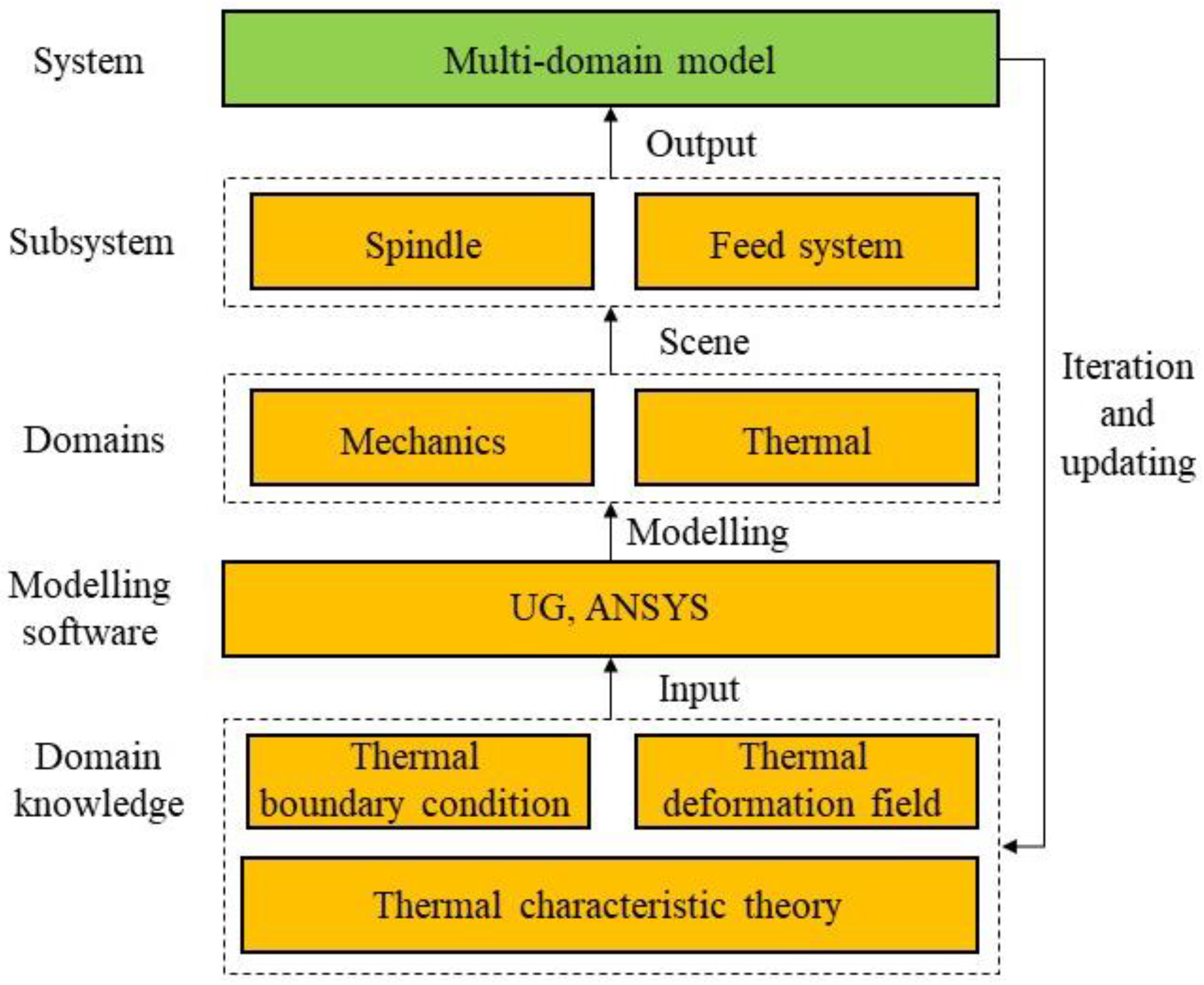
3.1. DT
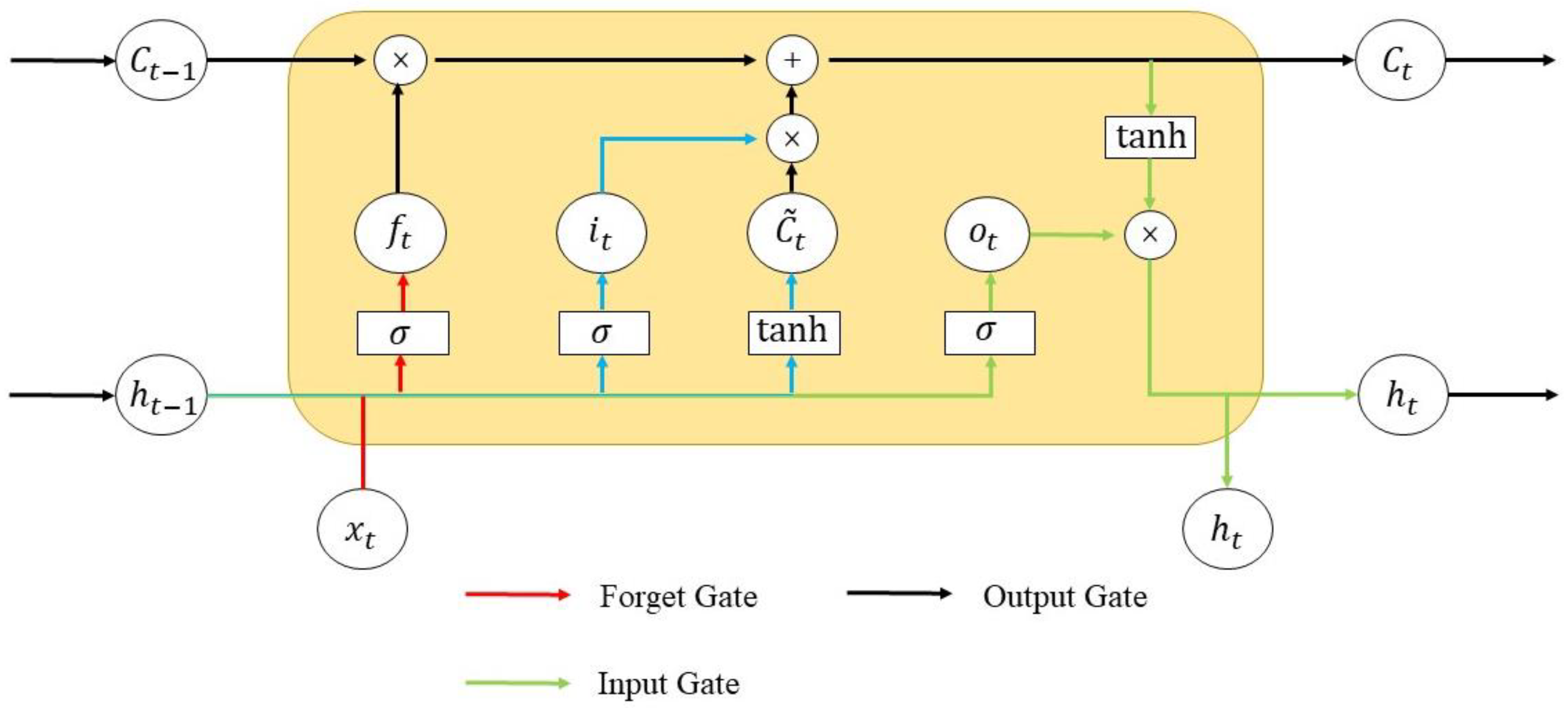
3.2. LSTM
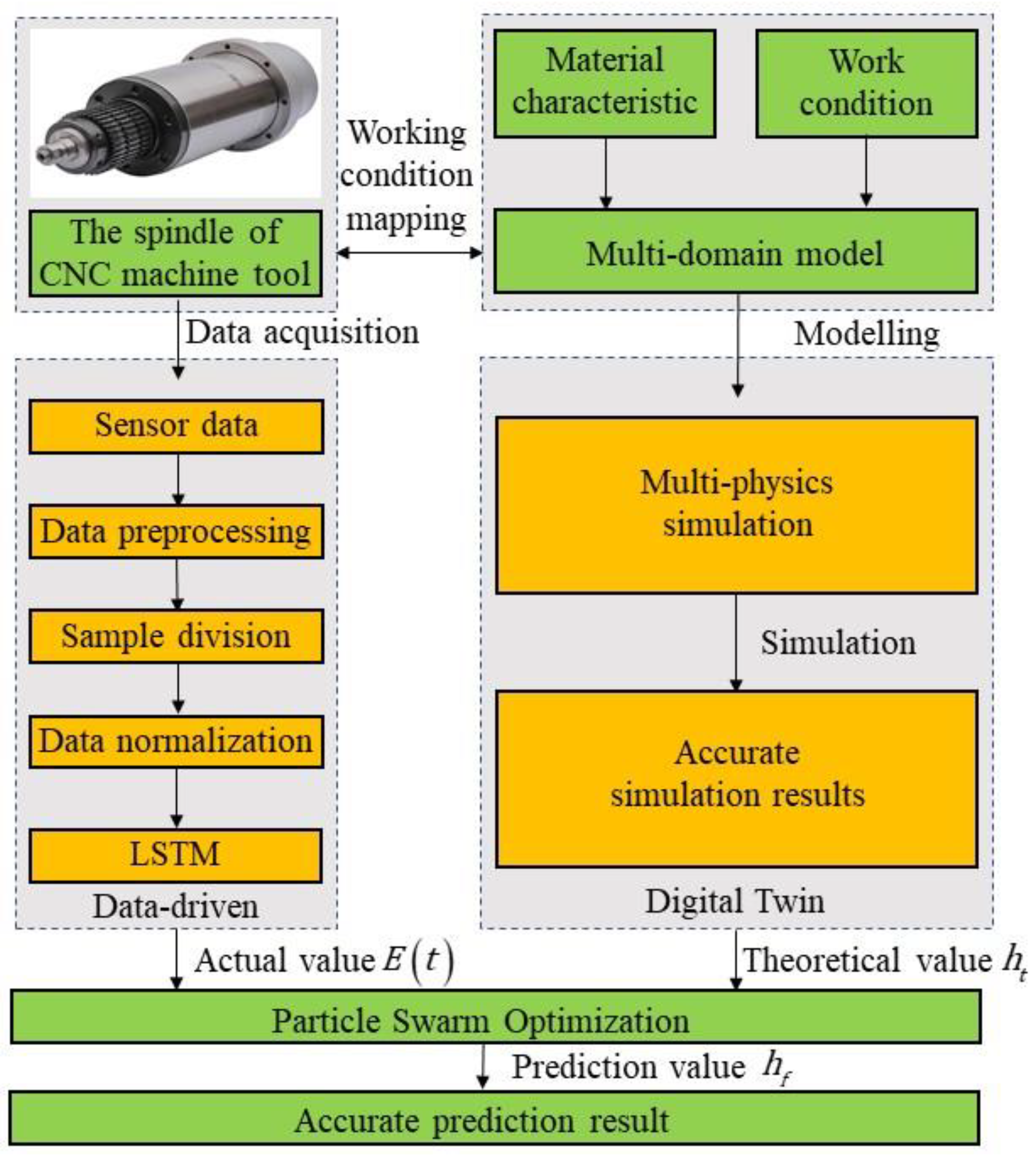
3.3. DT-LSTM
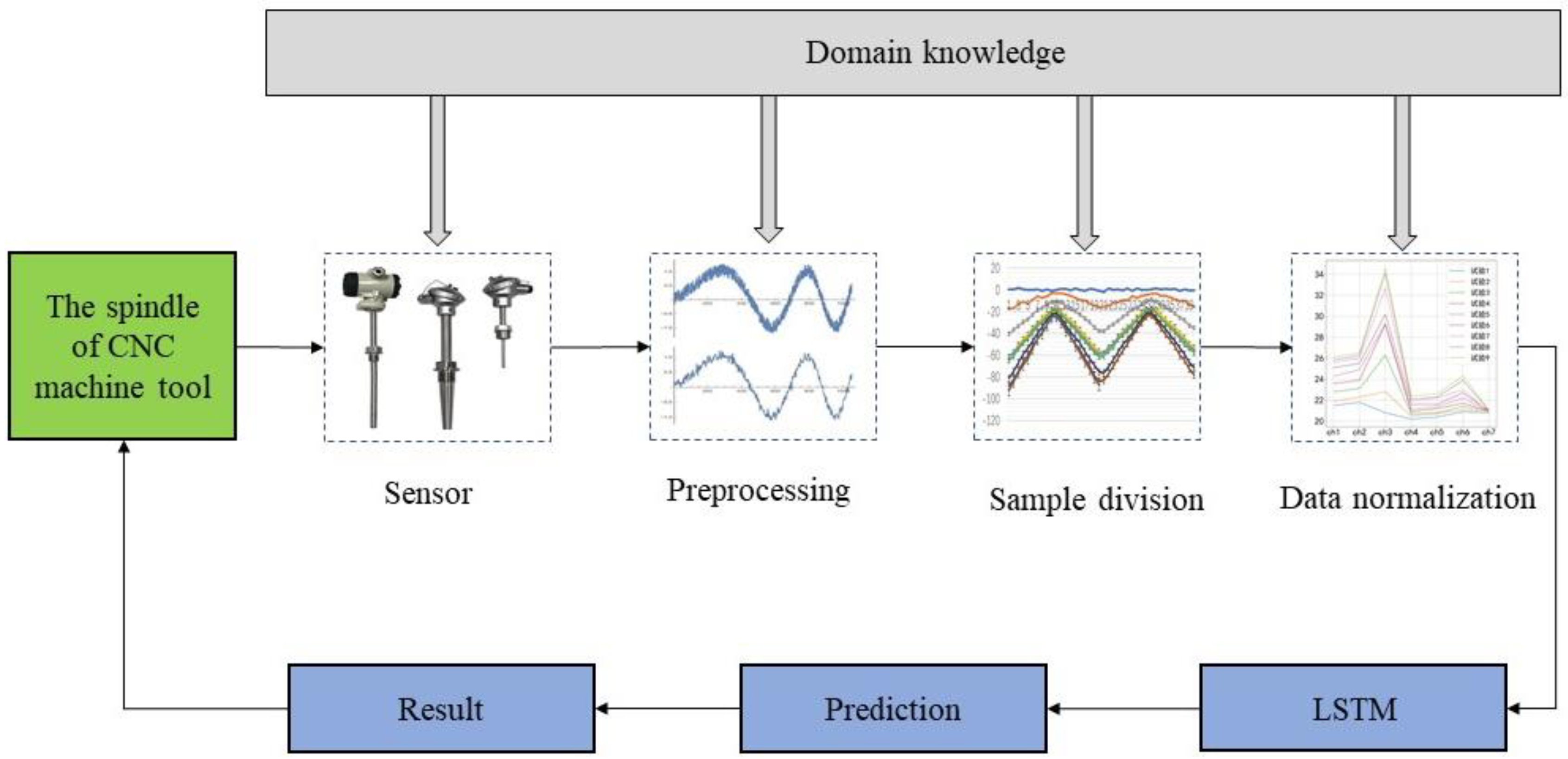
3.3.1. Framework
3.3.2. Implementation
- (1)
- The implementation of the DT model
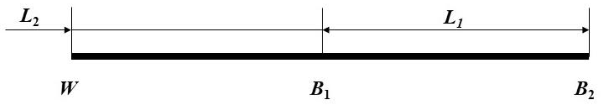
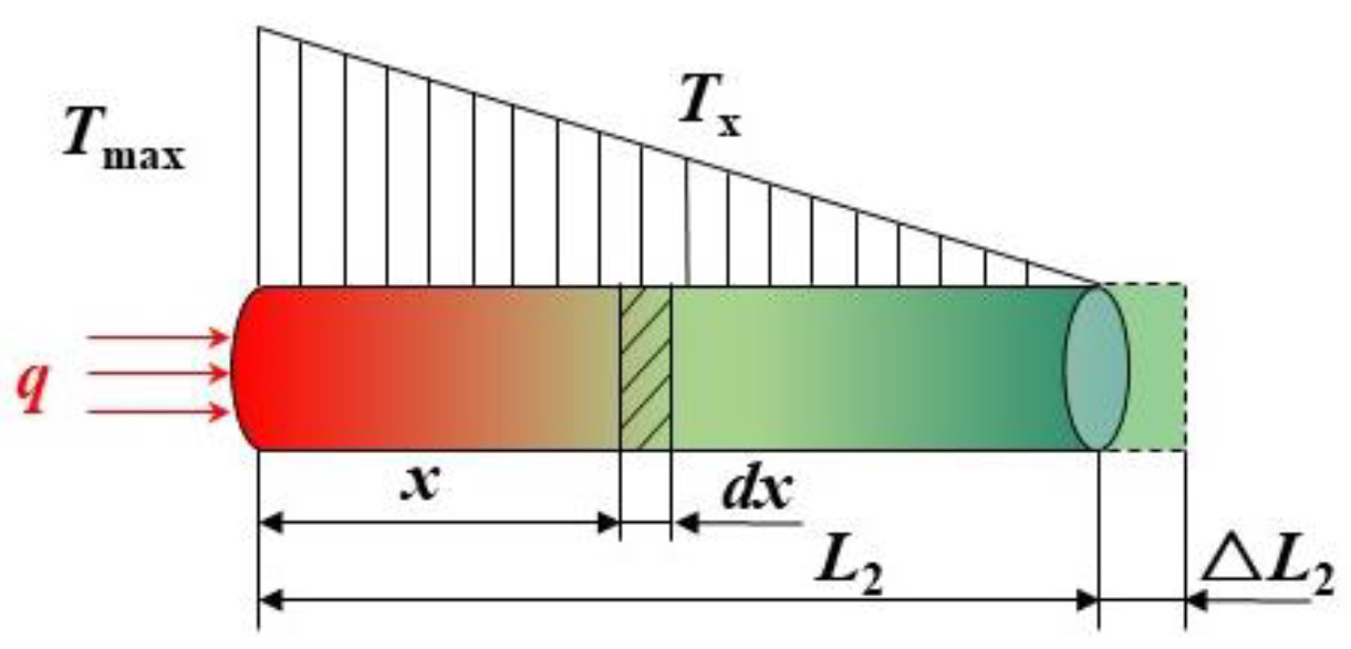
- Thermal boundary condition
- a.
- Bearing heat calculation
- b.
- Screw-nut heat calculation
- c.
- Convective heat transfer coefficient
- d.
- Thermal resistance calculation
- 2.
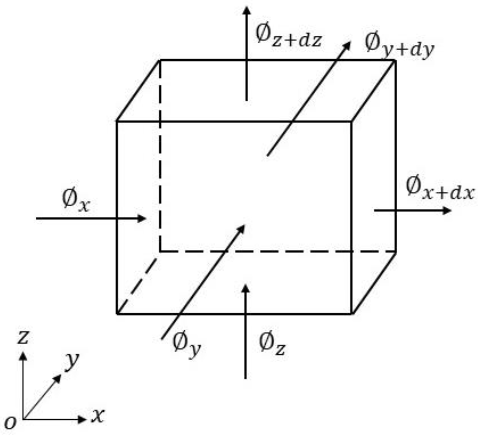
- Thermal characteristic analysis and modeling theory
- The temperature distribution at any time on the boundary of a given heat conductor [27].
- b.
- The heat flux density at any time on the boundary of a given heat conductor [27].
- c.
- The convective heat transfer coefficient between the boundary of the thermal conductor and the surface fluid, and the temperature of the surface fluid are given [27].
- 3.
- Mathematical model of the thermal deformation field
- (2)
- The implementation of the LSTM model
- (3)
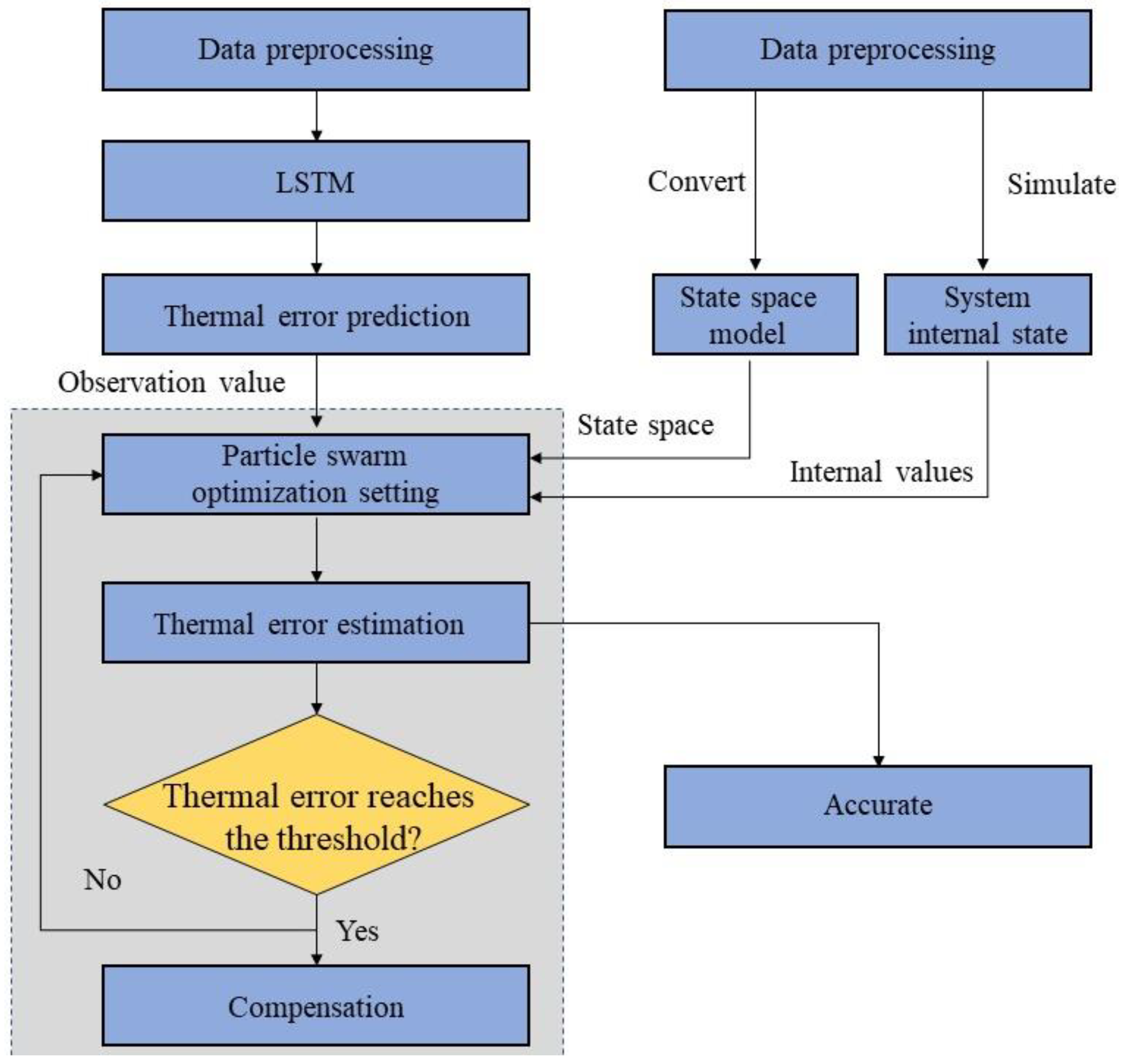
- The implementation of DT-LSTM
- An LSTM model for the CNCMT spindle system is established, and the predicted thermal error obtained from the model is used as an observation value.
- According to the temperature variation rules in the DT model, it is converted into a temperature space model for initialization based on the fusion algorithm, and the internal state of the system is calculated using model simulation.
- The fusion algorithm is initialized based on the temperature space model, and the observed values are used to modify the theoretical values obtained from the system model simulation and reasoning. We can obtain more accurate thermal error prediction values.
- We judge whether the thermal error reaches the threshold value based on the analysis results of the fusion algorithm. If the thermal error reaches the threshold value, we should make appropriate compensation. Otherwise, return to ii to repeat the iteration.
4. Case Study
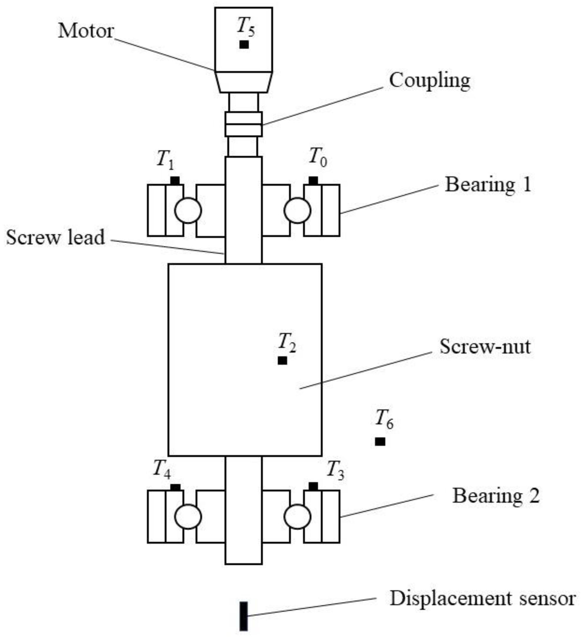
4.1. Design of Experiment Platform
4.2. The Optimization of the Temperature Measurement Points
4.3. DT-LSTM-based Thermal Error Prediction Approach for CNCMT Spindle
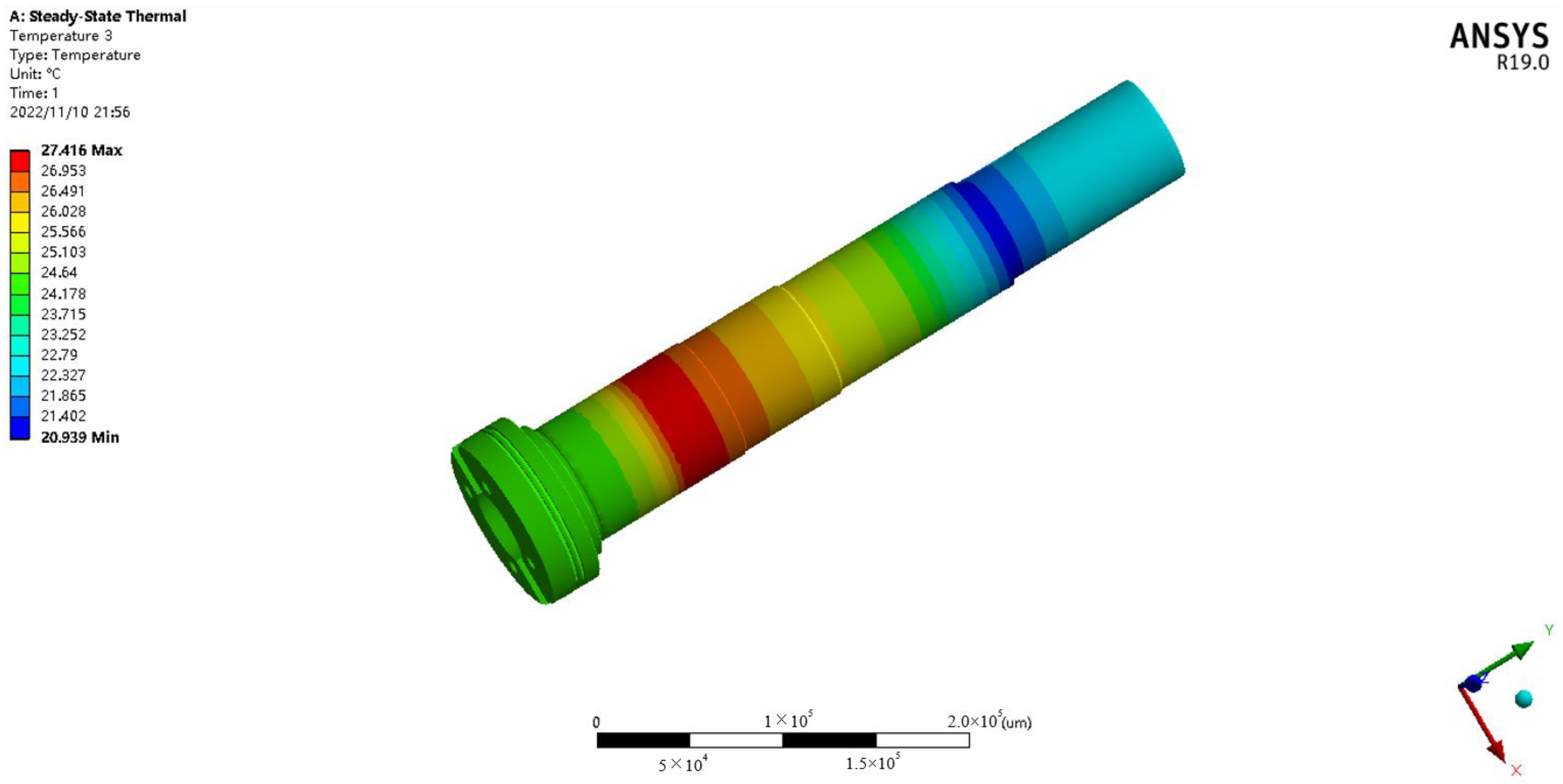
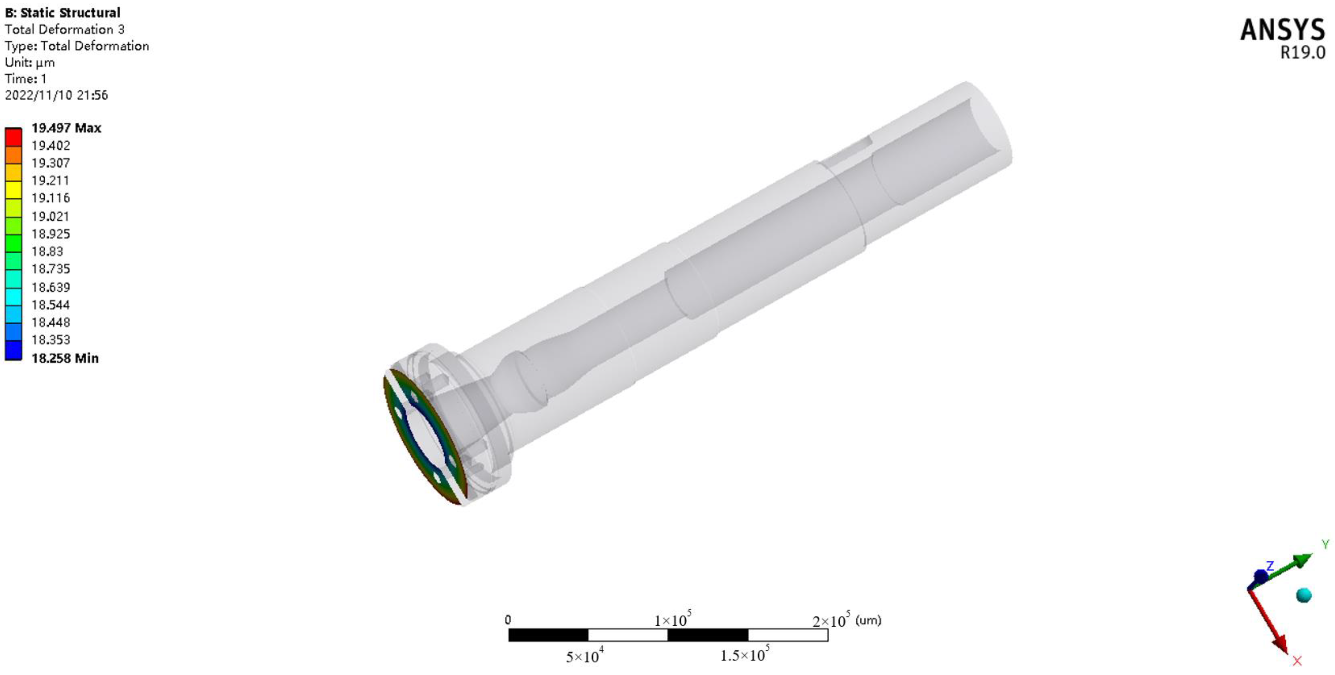
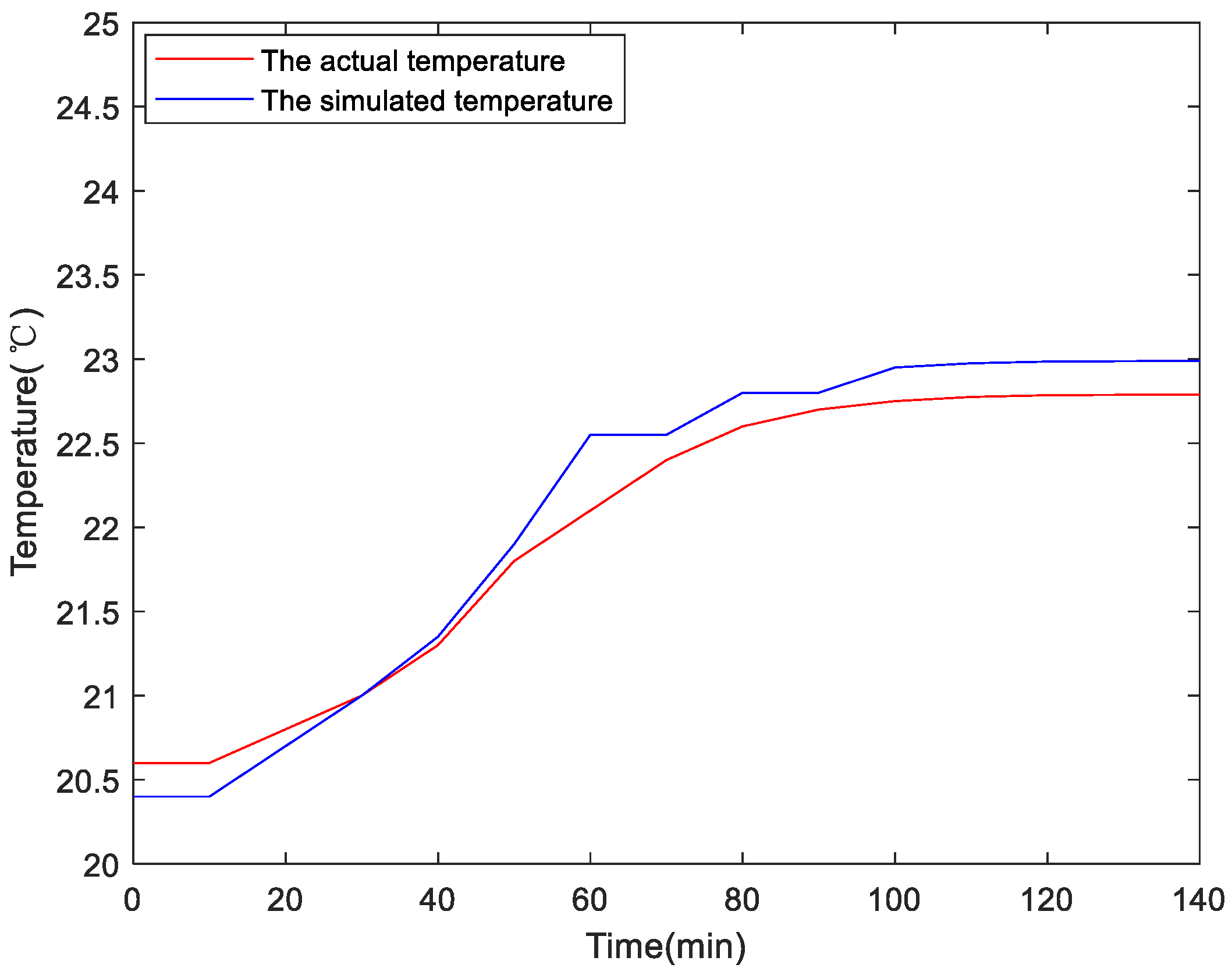
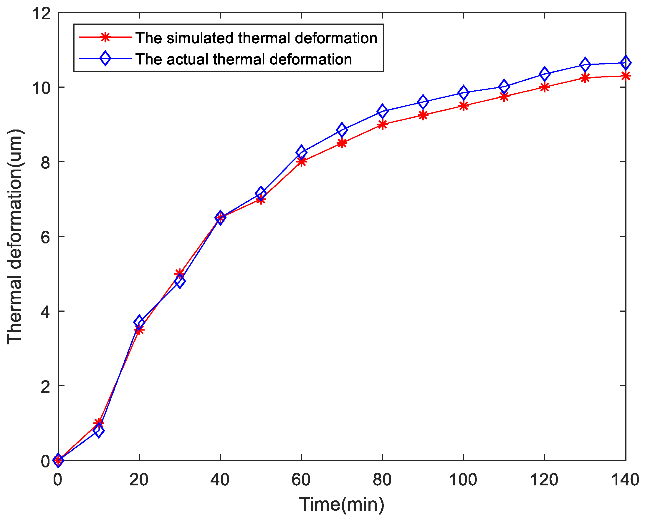
4.3.1. The Realization of the DT Model
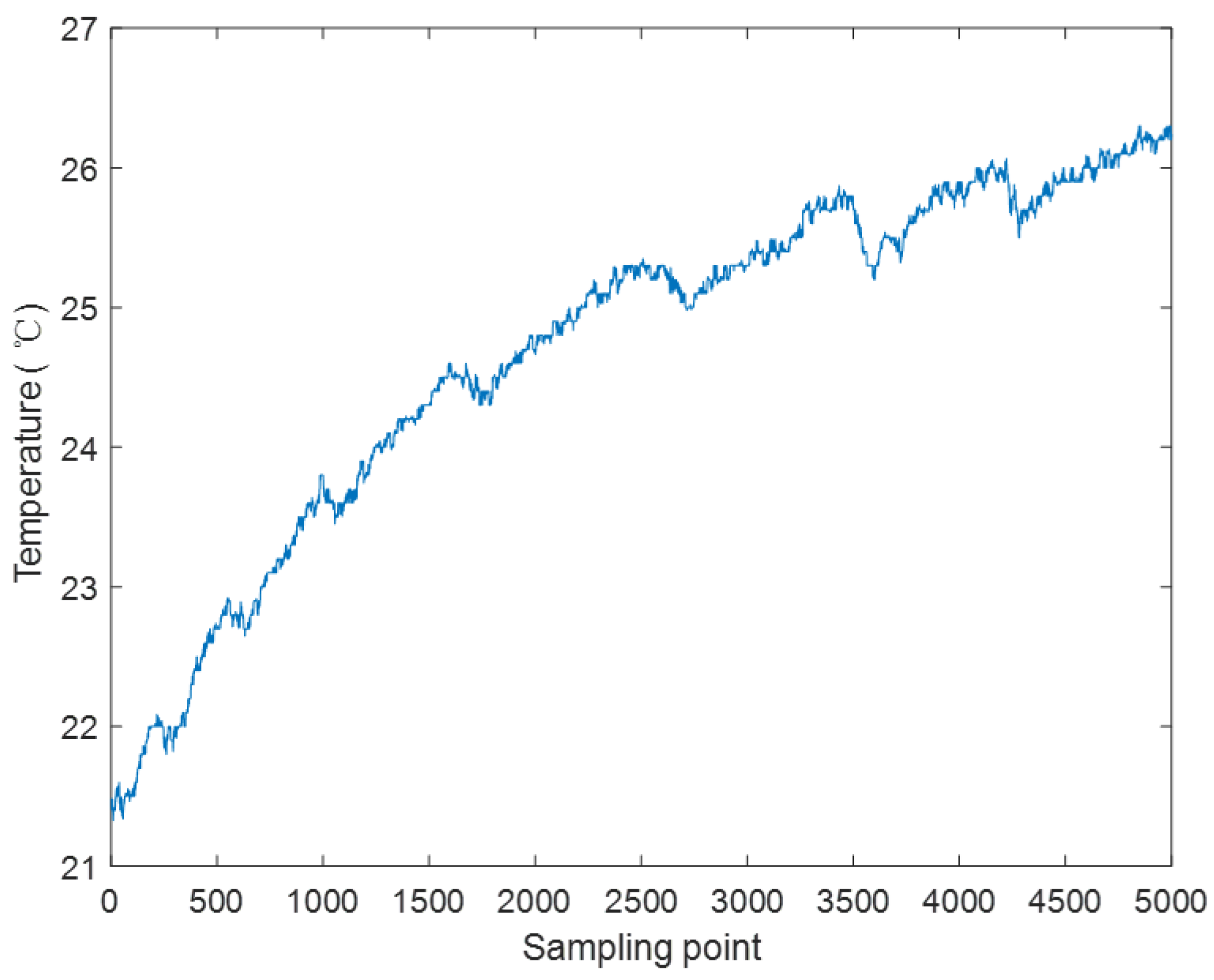
4.3.2. The Realization of the LSTM Model
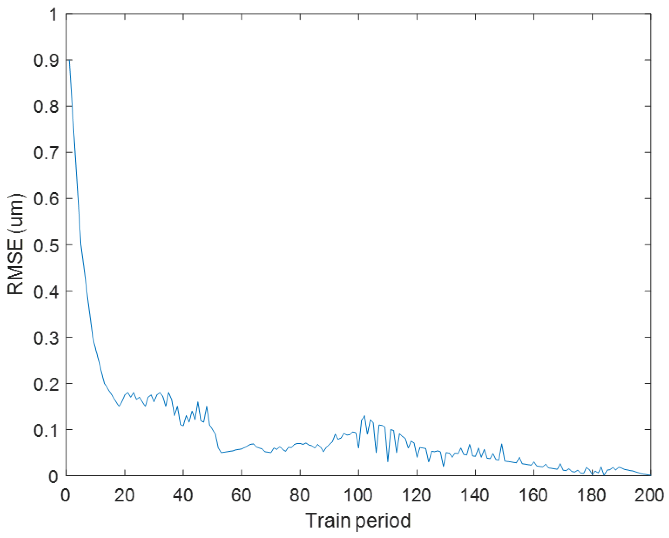
4.3.3. The Realization of DT-LSTM
| Algorithm 1. DT-LSTM for the CNCMT spindle’s thermal error prediction |
| Input: The theoretical prediction value of DT and the actual prediction value of LSTM |
| Output: The particles prediction value |
| (1) Initialize the parameters and particles |
| (2) |
| (3) for 1 = 1:150 |
| (4) Sample from (2) |
| (5) Calculate the thermal error prediction value of particles by (3) |
| (6) Calculate the weight of each particleend |
| (7) Normalize the weight |
| (8) Resample according to the normalized weight |
| (9) Output the CNCMT spindle’s thermal error prediction value |
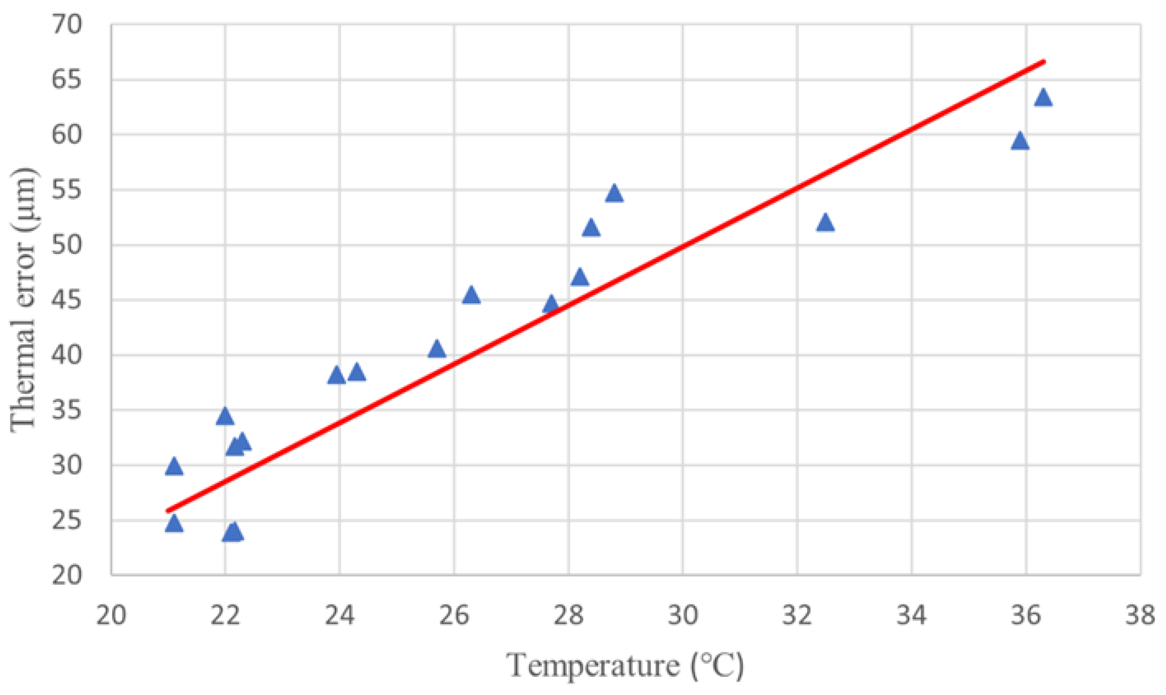
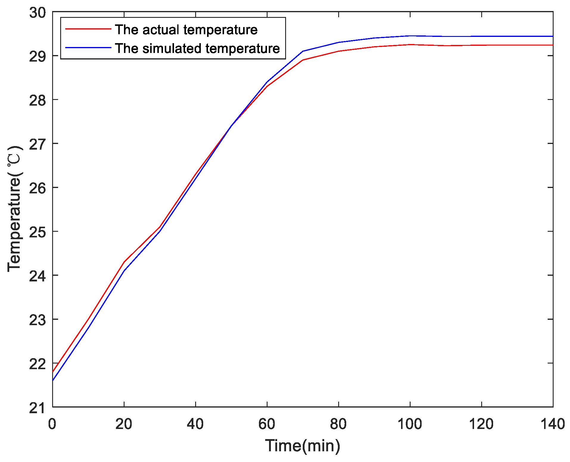
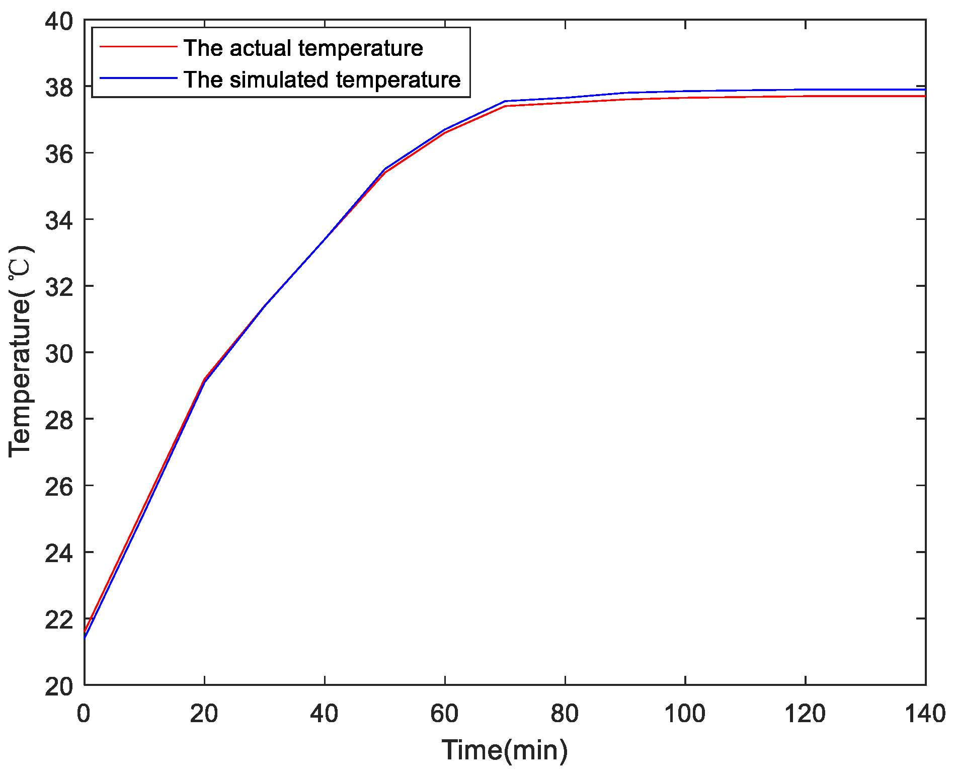
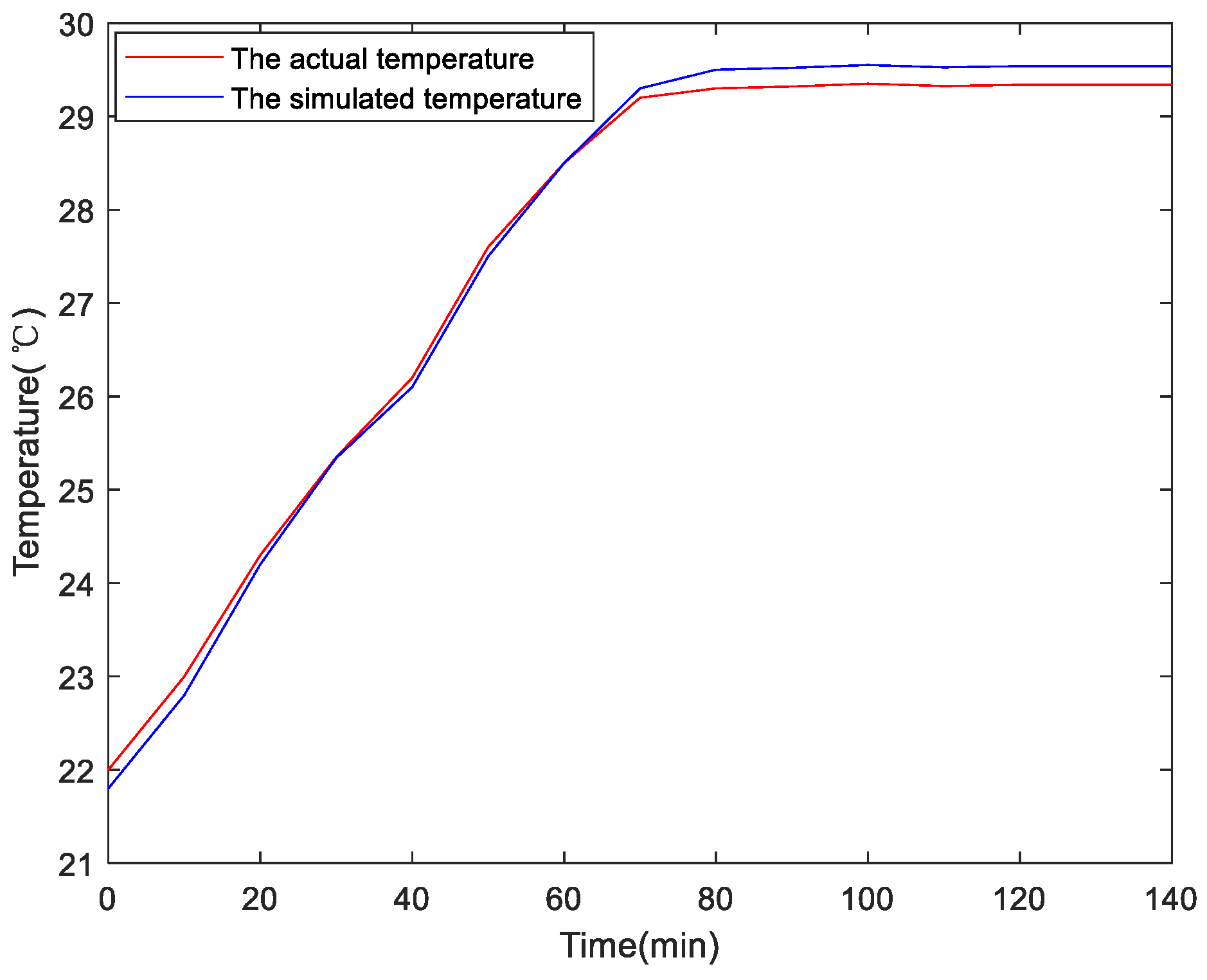
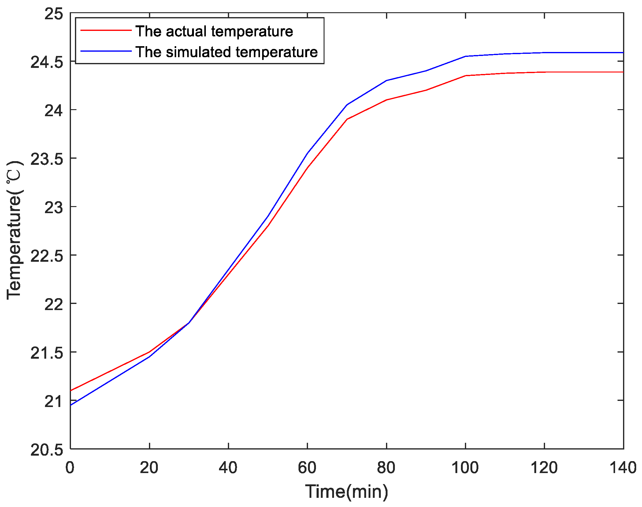
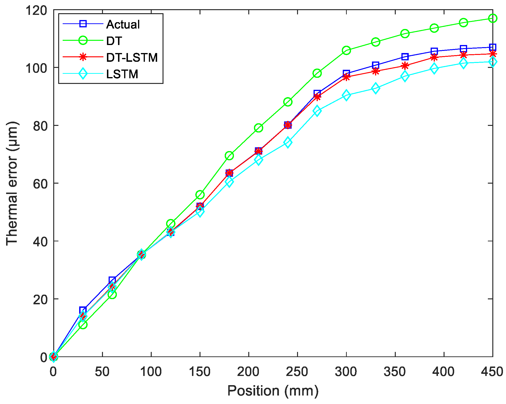
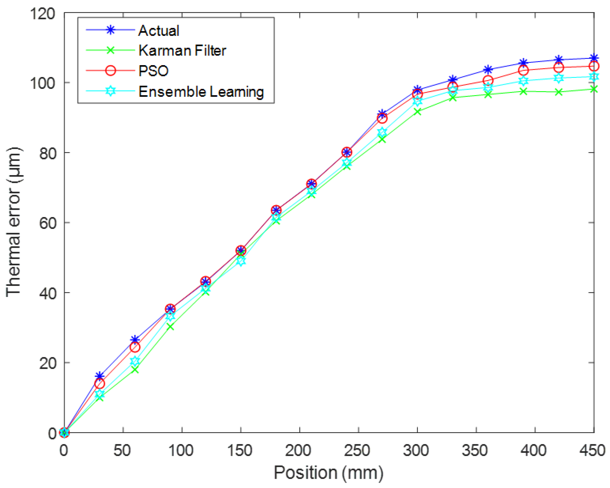
4.4. The Analysis of Experiment Result
5. Conclusions
Author Contributions
Funding
Data Availability Statement
Conflicts of Interest
References
- Li, Y.; Tian, H.; Liu, D.; Lu, Q.B. Thermal error analysis of five-axis machine tools based on five-point test method. Lubricants 2022, 10, 122. [Google Scholar] [CrossRef]
- Peng, J.; Yin, M.; Cao, L.; Liao, Q.; Wang, L.; Yin, G. Study on the spindle axial thermal error of a five-axis machining center considering the thermal bending effect. Precis. Eng. 2022, 75, 210–226. [Google Scholar] [CrossRef]
- Ouerhani, N.; Loehr, B.; Rizzotti-Kaddouri, A.; Santo De Pinho, D.; Limat, A.; Schinderholz, P. Data-driven thermal deviation prediction in turning machine-tool-a comparative analysis of machine learning algorithms. Procedia Comput. Sci. 2022, 200, 185–193. [Google Scholar] [CrossRef]
- Zimmermann, N.; Lang, S.; Blaser, P.; Mayr, J. Adaptive input selection for thermal error compensation models. CIRP Ann. 2020, 69, 485–488. [Google Scholar] [CrossRef]
- Liang, Y.C.; Li, W.D.; Lou, P.; Hu, J.M. Thermal error prediction for heavy-duty CNC machines enabled by long short-term memory networks and fog-cloud architecture. J. Manuf. Syst. 2022, 62, 950–963. [Google Scholar] [CrossRef]
- Li, Y.; Yu, M.; Bai, Y.; Hou, Z.; Wu, W. A review of thermal error modeling methods for machine tools. Appl. Sci. 2021, 11, 5216. [Google Scholar] [CrossRef]
- Li, Z.; Wang, B.; Zhu, B.; Wang, Q.; Zhu, W. Thermal error modeling of electrical spindle based on optimized ELM with marine predator algorithm. Case Stud. Therm. Eng. 2022, 38, 102326. [Google Scholar] [CrossRef]
- Liao, Q.; Yin, Q.; Xie, L.; Yin, G. Improved exponential model for thermal error modeling of machine-tool spindle based on fruit fly optimization algorithm. Proc. Inst. Mech. Eng. C J. Mech. 2022, 236, 6912–6922. [Google Scholar] [CrossRef]
- Kumar, T.S.; Kurian, C.P. Real-time data based thermal comfort prediction leading to temperature setpoint control. J. Ambient Intell. Hum. Comput. 2022, 1–12. [Google Scholar] [CrossRef]
- Li, Z.; Fan, K.; Yang, J.; Zhang, Y. Time-varying positioning error modeling and compensation for ball screw systems based on simulation and experimental analysis. Int. J. Adv. Manuf. Technol. 2014, 73, 773–782. [Google Scholar] [CrossRef]
- Abdulshahed, A.M.; Longstaff, A.P.; Fletcher, S.; Potdar, A. Thermal error modelling of a gantry-type 5-axis machine tool using a grey neural network model. J. Manuf. Syst. 2016, 41, 130–142. [Google Scholar] [CrossRef]
- Zhu, X.; Liu, Q.; Zhang, X.; Jiang, X.; Lou, P. Robustness analysis of the thermal error model for a CNC machine tool. In Proceedings of the 2016 8th International Conference on Intelligent Human-Machine Systems and Cybernetics (IHMSC), Cairo, Egypt, 27–28 August 2016; pp. 510–513. [Google Scholar]
- Yang, J.; Zhang, D.; Mei, X.; Zhao, L.; Ma, C.; Shi, H. Thermal error simulation and compensation in a jig-boring machine equipped with a dual-drive servo feed system. Proc. Inst. Mech. Eng. B J. Eng. 2015, 229, 43–63. [Google Scholar] [CrossRef]
- Liu, J.; Gui, H.; Ma, C. Digital twin system of thermal error control for a large-size gear profile grinder enabled by gated recurrent unit. J. Ambient Intell. Hum. Comput. 2023, 14, 1269–1295. [Google Scholar] [CrossRef]
- Ma, C.; Gui, H.; Liu, J. Self learning-empowered thermal error control method of precision machine tools based on digital twin. J. Intell. Manuf. 2023, 34, 695–717. [Google Scholar] [CrossRef]
- Xiao, J.; Fan, K. Research on the digital twin for thermal characteristics of motorized spindle. Int. J. Adv. Manuf. Technol. 2022, 119, 5107–5118. [Google Scholar] [CrossRef]
- Liu, K.; Song, L.; Han, W.; Cui, Y.; Wang, Y. Time-varying error prediction and compensation for movement axis of CNC machine tool based on digital twin. IEEE Trans. Ind. Inform. 2021, 18, 109–118. [Google Scholar] [CrossRef]
- Yi, H.; Fan, K. Co-simulation-based digital twin for thermal characteristics of motorized spindle. Int. J. Adv. Manuf. Technol. 2023, 125, 4725–4737. [Google Scholar] [CrossRef]
- Liu, J.; Ma, C.; Gui, H.; Wang, S. A four-terminal-architecture cloud-edge-based digital twin system for thermal error control of key machining equipment in production lines. Mech. Syst. Signal Process. 2022, 166, 108488. [Google Scholar] [CrossRef]
- Lunev, A.; Lauerer, A.; Zborovskii, V.; Léonard, F. Digital twin of a laser flash experiment helps to assess the thermal performance of metal foams. Int. J. Therm. Sci. 2022, 181, 107743. [Google Scholar] [CrossRef]
- Kuprat, J.; Pascal, Y.; Liserre, M. Real-Time thermal characterization of power semiconductors using a PSO-based digital twin approach. In Proceedings of the 2022 24th European Conference on Power Electronics and Applications (EPE’22 ECCE Europe), Hanover, Germany, 5–9 September 2022; pp. 1–8. [Google Scholar]
- Liu, R.J.; Li, H.S.; Lv, Z.H. Modeling methods of 3D model in digital twins. CMES Comp. Model. Eng. 2023, 136, 985–1022. [Google Scholar] [CrossRef]
- Grieves, M.W. Product lifecycle management: The new paradigm for enterprises. Int. J. Prod. Dev. 2005, 2, 71–84. [Google Scholar] [CrossRef]
- Tao, F.; Zhang, H.; Liu, A.; Nee, A.Y. Digital twin in industry: State-of-the-art. IEEE Trans. Ind. Inform. 2018, 15, 2405–2415. [Google Scholar] [CrossRef]
- Smagulova, K.; James, A.P. A survey on LSTM memristive neural network architectures and applications. Eur. Phys. J. Spec. Top. 2019, 228, 2313–2324. [Google Scholar] [CrossRef]
- Korstanje, J. LSTM RNNs. In Advanced Forecasting with Python: With State-of-the-Art-Models Including LSTMs, Facebook’s Prophet, and Smazon’s DeepAR Apress; Apress: Berkeley, CA, USA, 2021; pp. 243–251. [Google Scholar]
- Pope, J.E.; Pope, E. Rule of Thumb for Mechanical Engineers-A Manual of Quick, Accurate Solutions to Everyday Mechanical Engineering Problems; Gulf Professional Publishing: Houston, TX, USA, 1997; pp. 18–50. [Google Scholar]
- Chen, Z.C.; Chen, Z.N. Termal Characteristics Foundation of Machine Tools; Machinery Industry Press: Beijing, China, 1989. [Google Scholar]
- Ruspini, E.H.; Bezdek, J.C.; Keller, J.M. Fuzzy clustering: A historical perspective. IEEE Comput. Intell. Mag. 2019, 14, 45–55. [Google Scholar] [CrossRef]
- Fang, B.; Zhang, J.; Hong, J.; Yan, K. Research on the nonlinear stiffness characteristics of double-row angular contact ball bearings under different working conditions. Lubricants 2023, 11, 44. [Google Scholar] [CrossRef]
- Ma, S.; Yin, Y.; Chao, B.; Yan, K.; Fang, B.; Hong, J. A real-time coupling model of bearing-rotor system based on semi-flexible body element. Int. J. Mech. Sci. 2023, 245, 108098. [Google Scholar] [CrossRef]


| T0 | T1 | T2 | T3 | T4 | T5 | T6 |
|---|---|---|---|---|---|---|
| Bearing 1 | Bearing 1 | Screw-nut | Bearing 2 | Bearing 2 | Motor | Surrounding |
| Temperature Measurement Point | Correlation Coefficient | Temperature Measurement Point | Correlation Coefficient |
|---|---|---|---|
| T0 | 0.9498 | T4 | 0.9565 |
| T1 | 0.9489 | T5 | 0.8866 |
| T2 | 0.9503 | T6 | 0.8815 |
| T3 | 0.9555 |
| Part | Spindle | Bearing |
|---|---|---|
| Material | GCr15SiMn | GCr15 |
| Density/(kg/m3) | 7810 | 7830 |
| Modulus of elasticity E/Pa | 2.06 × 10¹¹ | 2.19 × 10¹¹ |
| Poisson’s ratio μ | 0.3 | 0.3 |
| Specific heat capacity C/(J·(kg·K)−1) | 460 | 160 |
| Thermal conductivity/(W·(m·K)−1) | 60.5 | 81 |
| Coefficient of thermal expansion | 1.2 × 10⁻⁵ | 1.25 × 10⁻⁵ |
| Model Structure | LSTM Two-Layer Maximum Residual Error (μm) | LSTM Three-Layer Maximum Residual Error (μm) | LSTM Four-Layer Maximum Residual Error (μm) |
|---|---|---|---|
| eight hidden nodes | 10.5 | 7 | 16 |
| twelve hidden nodes | 6 | 9.5 | 19 |
| sixteen hidden nodes | 8 | 11.5 | 24.2 |
| twenty hidden nodes | 9.6 | 10 | 16.7 |
| Start Stage Accuracy | Middle Stage Accuracy | End Stage Accuracy | Average Accuracy | |
|---|---|---|---|---|
| DT | 91% | 88% | 82% | 87% |
| LSTM | 98% | 90% | 85% | 91% |
| DT-LSTM | 100% | 99% | 95% | 98% |
Disclaimer/Publisher’s Note: The statements, opinions and data contained in all publications are solely those of the individual author(s) and contributor(s) and not of MDPI and/or the editor(s). MDPI and/or the editor(s) disclaim responsibility for any injury to people or property resulting from any ideas, methods, instructions or products referred to in the content. |
© 2023 by the authors. Licensee MDPI, Basel, Switzerland. This article is an open access article distributed under the terms and conditions of the Creative Commons Attribution (CC BY) license (https://creativecommons.org/licenses/by/4.0/).
Share and Cite
Lu, Q.; Zhu, D.; Wang, M.; Li, M. Digital Twin-Driven Thermal Error Prediction for CNC Machine Tool Spindle. Lubricants 2023, 11, 219. https://doi.org/10.3390/lubricants11050219
Lu Q, Zhu D, Wang M, Li M. Digital Twin-Driven Thermal Error Prediction for CNC Machine Tool Spindle. Lubricants. 2023; 11(5):219. https://doi.org/10.3390/lubricants11050219
Chicago/Turabian StyleLu, Quanbo, Dong Zhu, Meng Wang, and Mei Li. 2023. "Digital Twin-Driven Thermal Error Prediction for CNC Machine Tool Spindle" Lubricants 11, no. 5: 219. https://doi.org/10.3390/lubricants11050219