Research on Nonconstant and Discontinuous Pumping Characteristics of the Concrete Pump Truck

 ,
,
Abstract
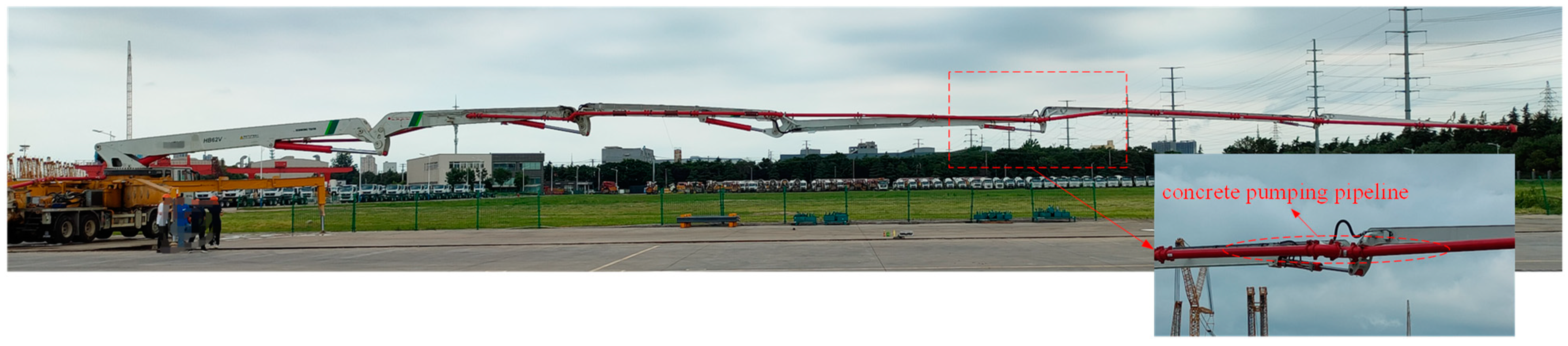
:1. Introduction
2. Concrete Pumping Model
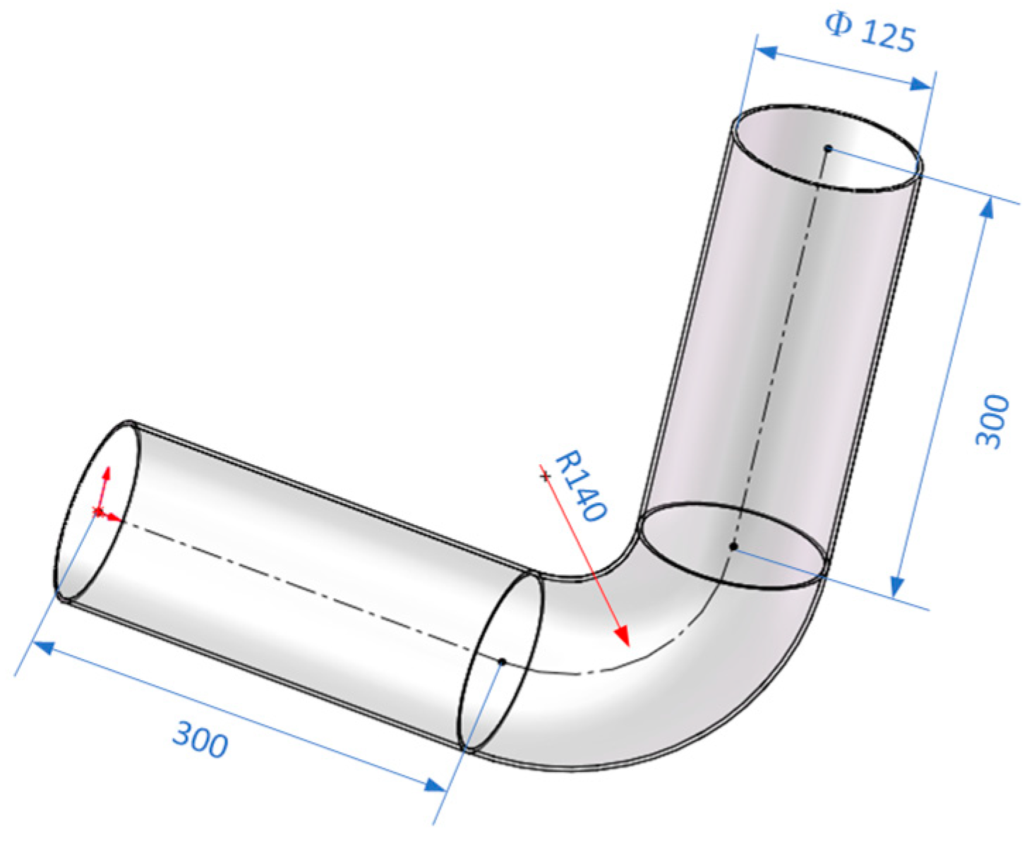
2.1. Concrete Pipeline Flow Model
2.2. Volume of Fluid (VOF) Model Control Equations
3. Rheological Characteristics of Nonconstant Concrete Pumping
3.1. Concrete Material Properties and Lubrication Layer Parameters
3.2. Force Analysis and Nonconstant Fluid Characteristic Simulation of Straight Pipe Pumping
3.3. Force Analysis and Nonconstant Fluid Characteristic Simulation of Elbow Pipe Pumping
4. Rheological Characteristics of Discontinuous Concrete Pumping
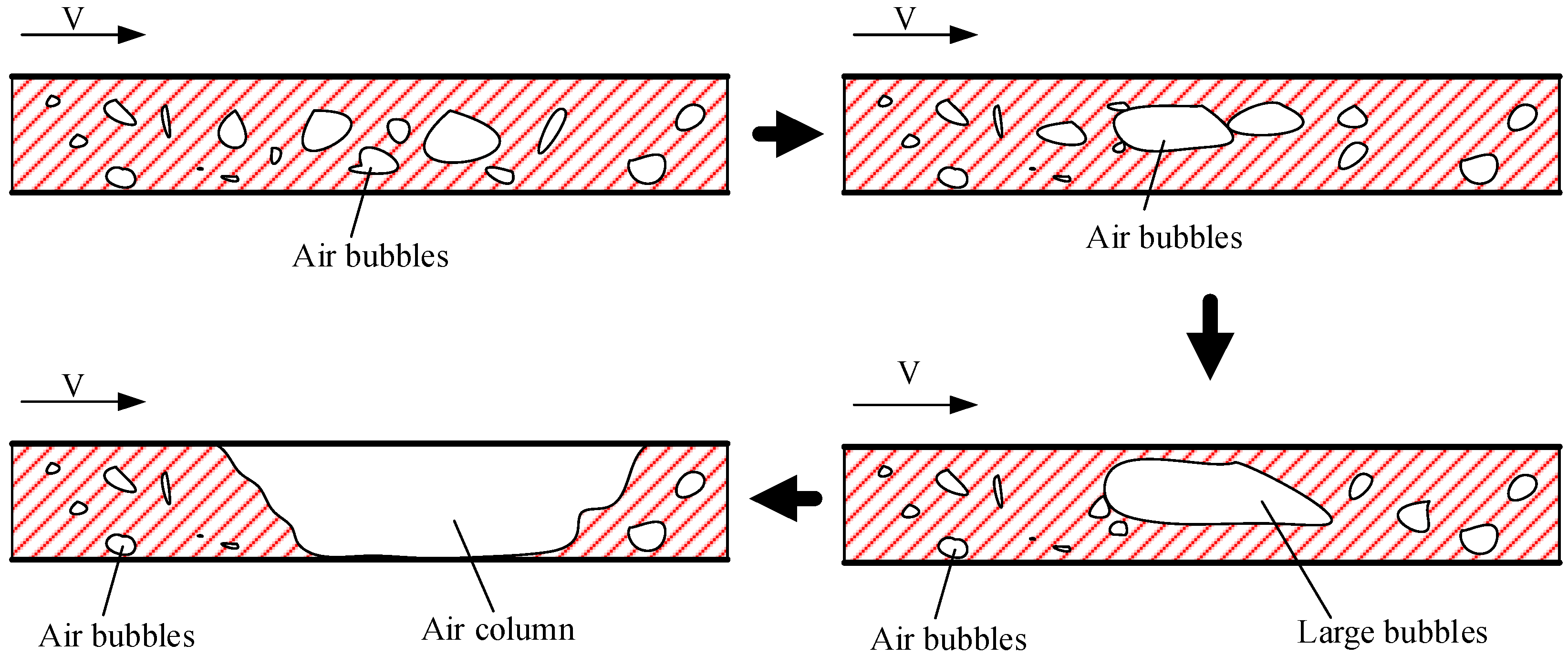
4.1. Discontinuous Flow Model
4.2. Pumping Characteristics of Concrete in the Straight Pipe
- (a)
- Pumping characteristics in the straight pipe under the influence of a single gas column
- (b)
- Pumping characteristics in the straight pipe under the influence of air column groups
4.3. Rheological Characteristics of Discontinuous Concrete Pumping in Elbow Pipes
5. Nonconstant and Discontinuous Concrete Pumping Characteristics
6. Conclusions
- 1.
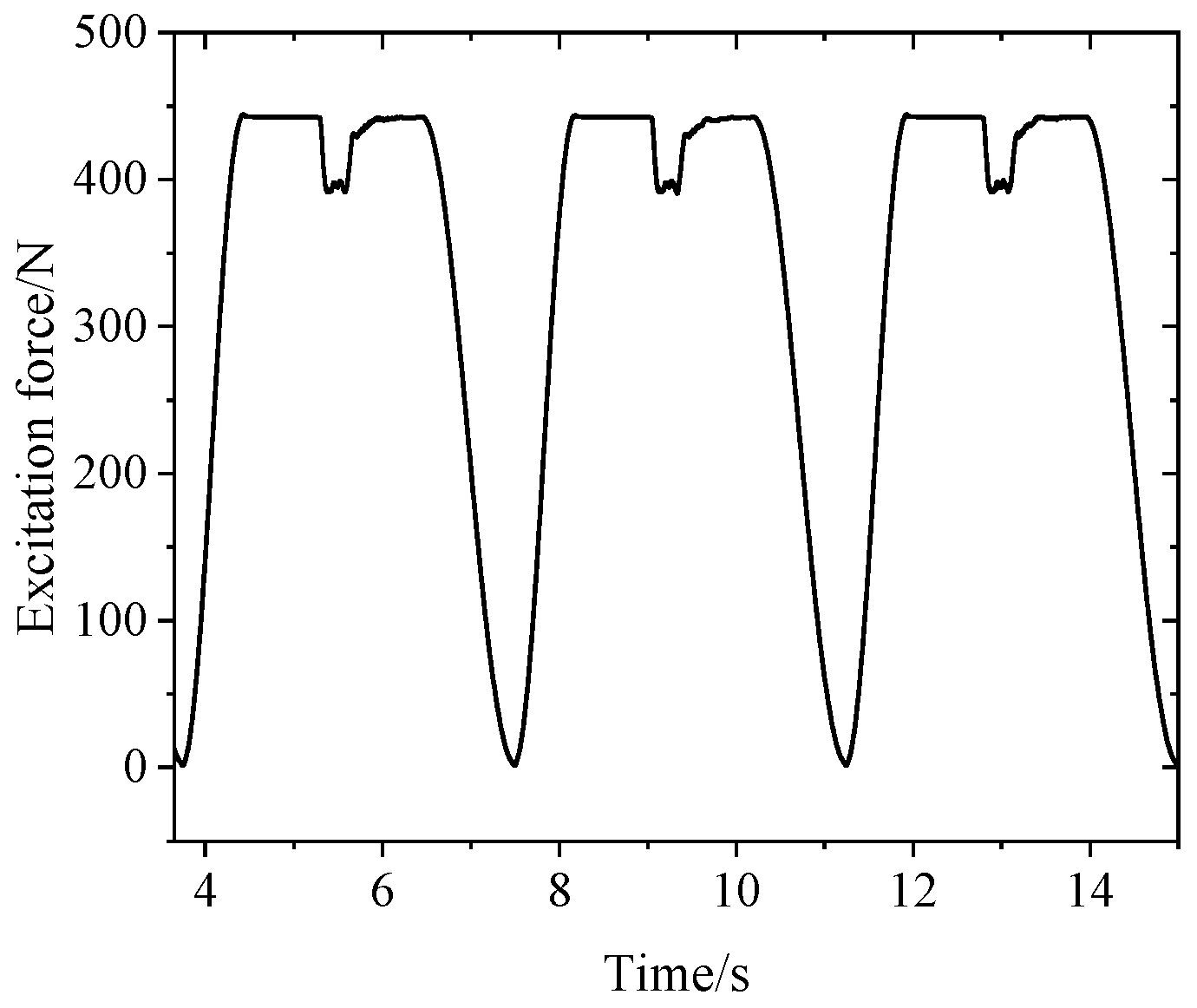
- For the nonconstant pumping of the concrete pump truck with two alternating cylinders, the pipeline pressure and the excitation force vary periodically with the pumping speed of concrete. With the change in pumping speed, the pipe pressure will have an obvious sudden peak in the initial stage of pumping; followed by the stable conveying stage, the pipe pressure is almost constant; and finally the reversing stage, the pressure will also decrease. The simulated pipeline pressure and the excitation force are basically consistent with the theoretical results.
- 2.
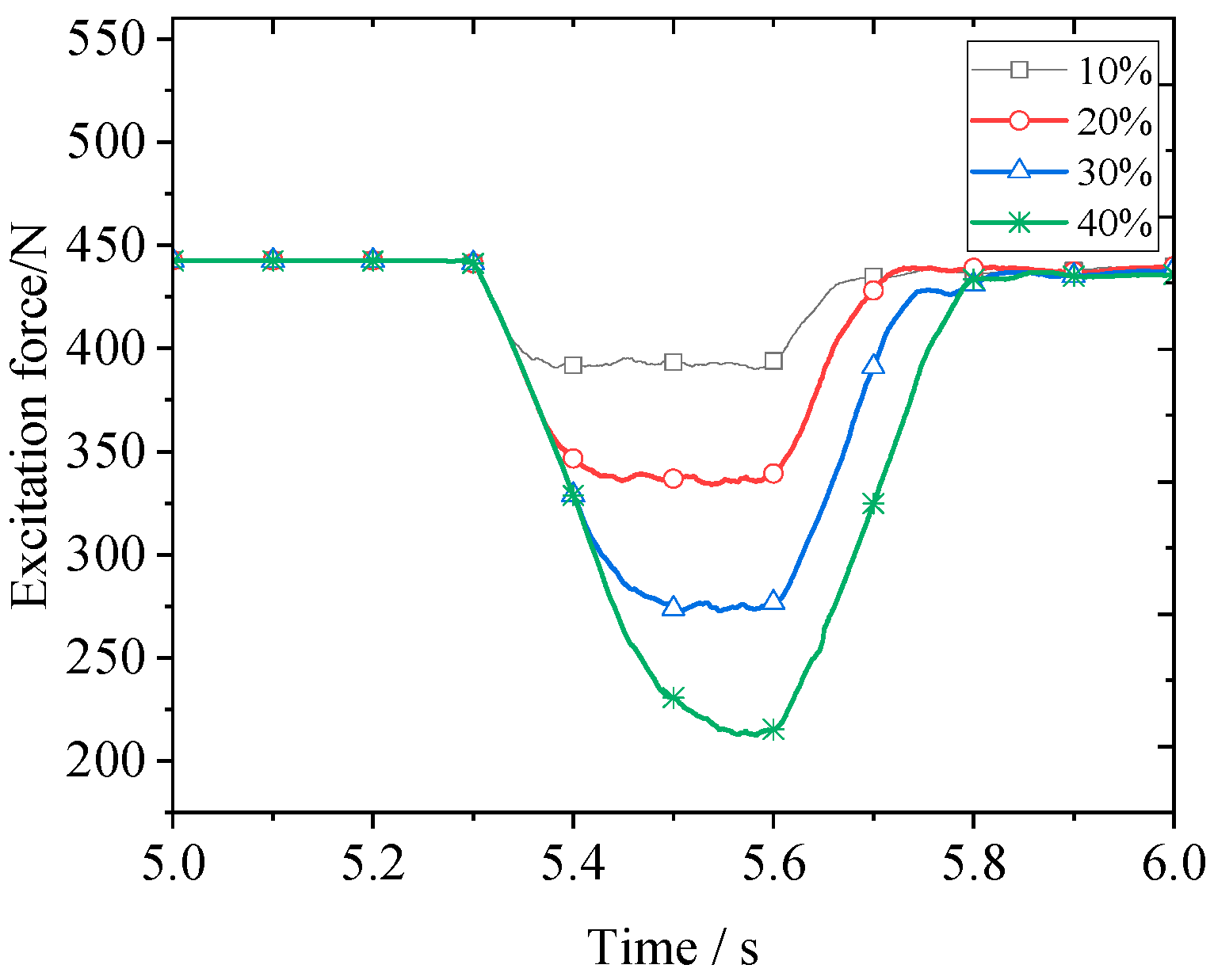
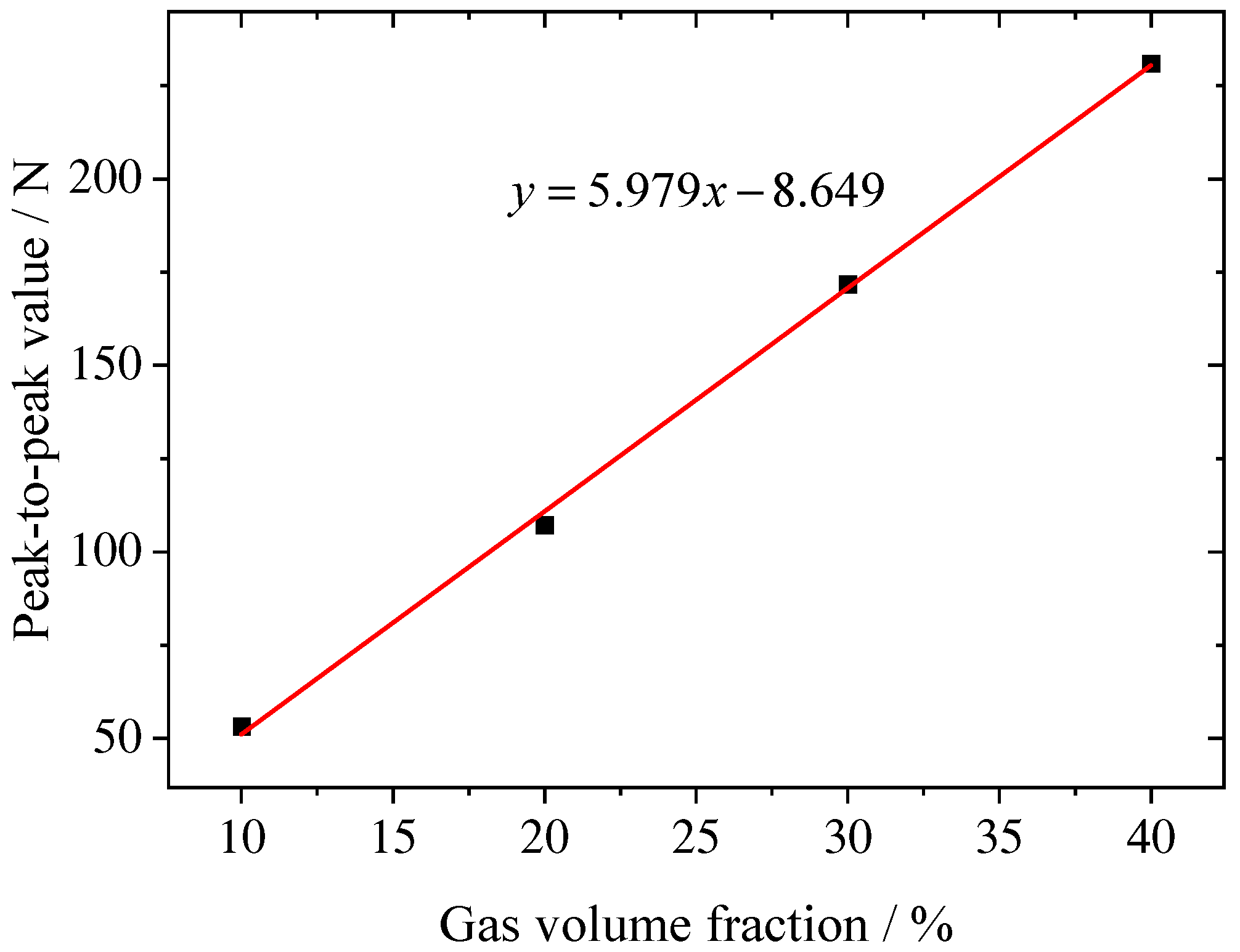
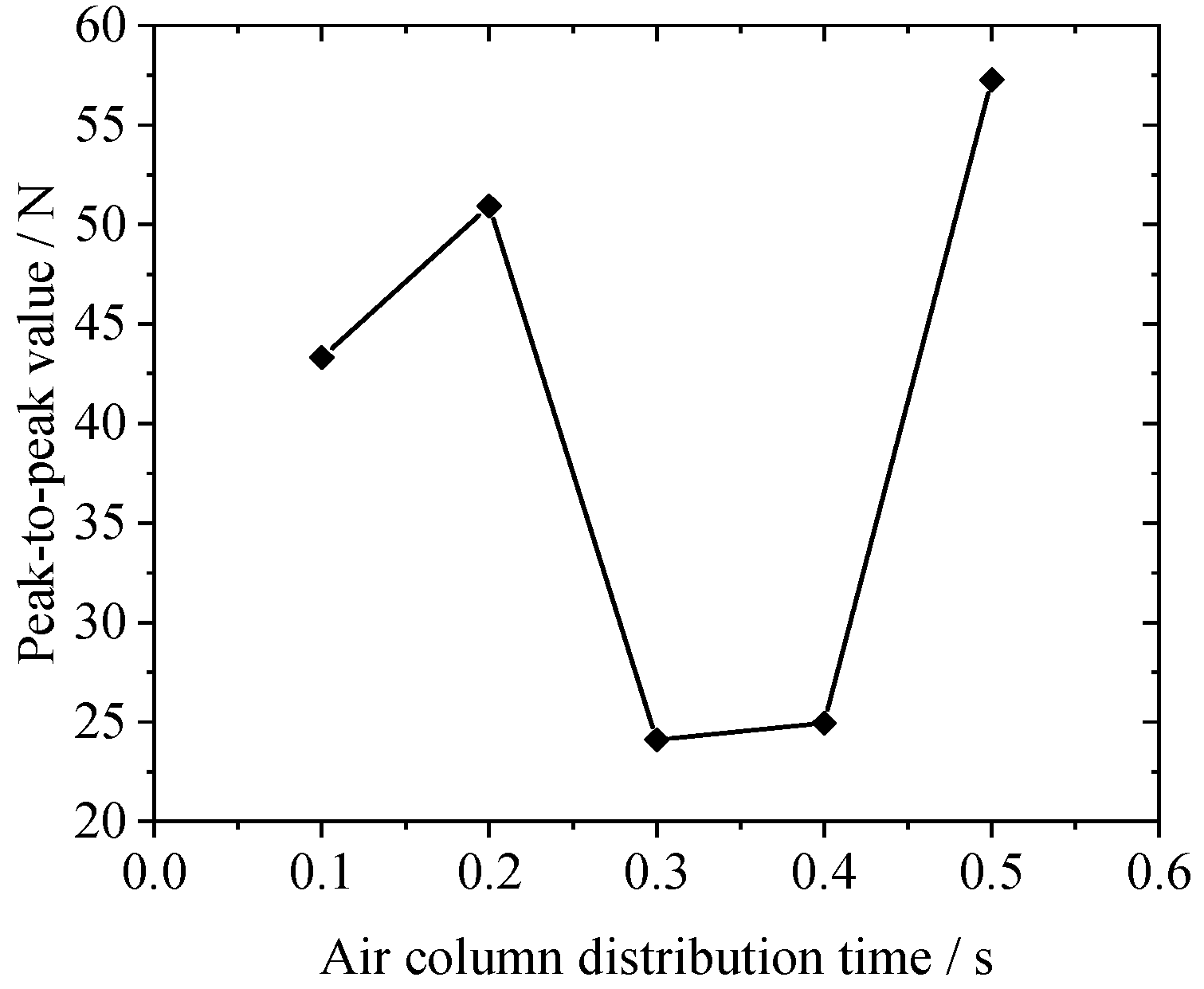
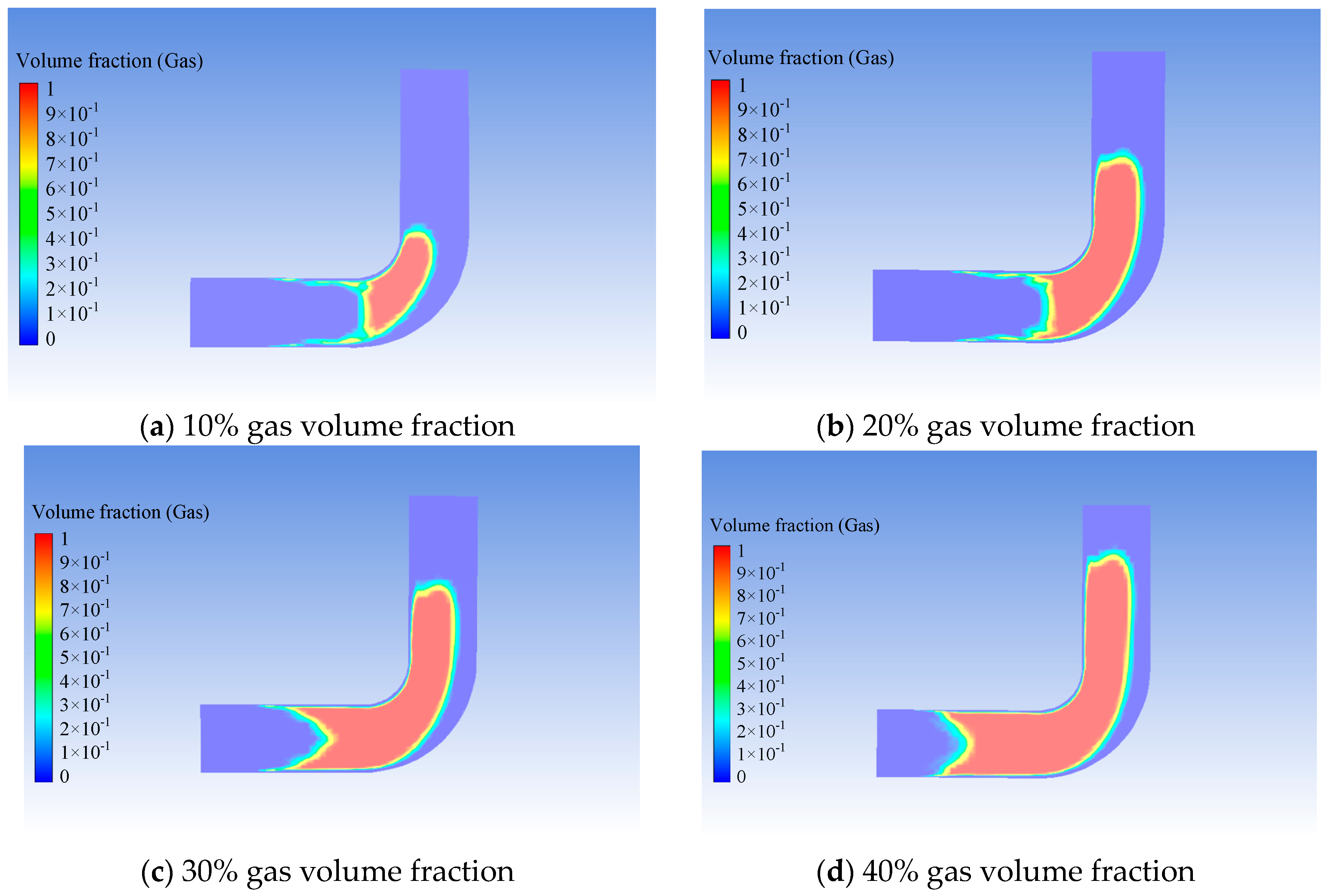
- For discontinuous concrete pumping caused by inadequate suction, the mean value of the pipe pressure and the wall excitation force is negatively correlated with the volume fraction of gas in the pipe under the condition that the volume fraction of gas does not exceed 40% of the total integral number of the pipe. The peak-to-peak value is positively correlated with the volume fraction when the gas column is distributed at low frequency. While the peak-to-peak value changes irregularly when the air columns are distributed at high frequency.
- 3.
- The air column will significantly increase the pipeline excitation force. The impact on the excitation of an elbow pipe is greater than the that of the straight pipe, and the impact law is more complex.
- 4.
- The pipe pressure of the nonconstant discontinuous concrete pumping model has a good consistency with the variation trend of pumping pressure of a real truck hydraulic cylinder, and the model can better reflect the nonconstant flow caused by the alternating pumping and the discontinuous flow caused by insufficient suction material. However, due to the limitations of experimental conditions, it is not yet possible to compare the specific simulation results with the experimental values.
Author Contributions
Funding
Data Availability Statement
Conflicts of Interest
References
- Wu, Y.Z.; Li, W.J.; Liu, Y.H. Fatigue life prediction for boom structure of concrete pump truck. Eng. Fail. Anal. 2016, 60, 176–187. [Google Scholar] [CrossRef]
- Tang, H.B.; Ren, W. Research on rigid-flexible coupling dynamic characteristics of boom system in concrete pump truck. Adv. Mech. Eng. 2015, 7, 1–7. [Google Scholar] [CrossRef]
- Zhaidarbek, B.; Tleubek, A.; Berdibek, G.; Wang, Y. Analytical predictions of concrete pumping, Extending the Khatib–Khayat model to Herschel–Bulkley and modified Bingham fluids. Cem. Concr. Res. 2023, 163, 107035. [Google Scholar] [CrossRef]
- Roussel, N.; Geiker, M.R.; Dufour, F.; Thrane, L.N.; Szabo, P. Computational modeling of concrete flow, General overview. Cem. Concr. Res. 2007, 37, 1298–1307. [Google Scholar] [CrossRef]
- Dufour, F.; Pijaudier-Cabot, G. Numerical modelling of concrete flow, homogeneous approach. Int. J. Numer. Anal. Methods Geomech. 2005, 29, 395–416. [Google Scholar] [CrossRef]
- Li, H.; Sun, D.; Wang, Z.; Huang, F.; Yi, Z.; Yang, Z.; Zhang, Y. A Review on the Pumping Behavior of Modern Concrete. J. Adv. Concr. Technol. 2020, 18, 352–363. [Google Scholar] [CrossRef]
- Kim, J.S.; Kwon, S.H.; Jang, K.P.; Choi, M.S. Concrete pumping prediction considering different measurement of the rheological properties. Constr. Build. Mater. 2018, 171, 493–503. [Google Scholar] [CrossRef]
- Jang, K.P.; Kwon, S.H.; Choi, M.S.; Kim, Y.J.; Park, C.K.; Shah, S.P. Experimental Observation on Variation of Rheological Properties during Concrete Pumping. Int. J. Concr. Struct. Mater. 2018, 12, 79. [Google Scholar] [CrossRef]
- Remond, S.; Pizette, P. A DEM hard-core soft-shell model for the simulation of concrete flow. Cem. Concr. Res. 2014, 58, 169–178. [Google Scholar] [CrossRef]
- Shyshko, S.; Mechtcherine, V. Developing a Discrete Element Model for simulating fresh concrete, Experimental investigation and modelling of interactions between discrete aggregate particles with fine mortar between them. Constr. Build. Mater. 2013, 47, 601–615. [Google Scholar] [CrossRef]
- Mechtcherine, V.; Shyshko, S. Simulating the behaviour of fresh concrete with the Distinct Element Meth—Deriving model parameters related to the yield stress. Cem. Concr. Compos. 2015, 55, 81–90. [Google Scholar] [CrossRef]
- Hao, J.; Jin, C.; Li, Y.; Wang, Z.; Liu, J.; Li, H. Simulation of Motion Behavior of Concrete in Pump Pipe by DEM. Adv. Civ. Eng. 2021, 2021, 3750589. [Google Scholar] [CrossRef]
- Jiang, S.; Chen, X.; Cao, G.; Tan, Y.; Xiao, X.; Zhou, Y.; Liu, S.; Tong, Z.; Wu, Y. Optimization of fresh concrete pumping pressure loss with CFD-DEM approach. Constr. Build. Mater. 2021, 276, 122204. [Google Scholar] [CrossRef]
- Jiang, S.; Zhang, W.; Chen, X.; Cao, G.; Tan, Y.; Xiao, X.; Liu, S.; Yu, Q.; Tong, Z. CFD-DEM simulation research on optimization of spatial attitude of concrete pumping boom based on evaluation of minimum pressure loss. Powder Technol. 2022, 403, 117365. [Google Scholar] [CrossRef]
- Wang, Z.G.; Hao, J.; Li, Y.; Tian, X. Simulation of Concrete Pumped in Horizontal Coil and Super High-Rise Building Based on CFD. J. Adv. Concr. Technol. 2022, 20, 328–341. [Google Scholar] [CrossRef]
- Le, H.D.; Kadri, E.H.; Aggoun, S.; Vierendeels, J.; Troch, P.; De Schutter, G. Effect of lubrication layer on velocity profile of concrete in a pumping pipe. Mater. Struct. 2015, 48, 3991–4003. [Google Scholar] [CrossRef]
- Secrieru, E.; Cotardo, D.; Mechtcherine, V.; Lohaus, L.; Schröfl, C.; Begemann, C. Changes in concrete properties during pumping and formation of lubricating material under pressure. Cem. Concr. Res. 2018, 108, 129–139. [Google Scholar] [CrossRef]
- Jang, K.P.; Choi, M.S. How affect the pipe length of pumping circuit on concrete pumping. Constr. Build. Mater. 2019, 208, 758–766. [Google Scholar] [CrossRef]
- Feys, D.; Khayat, K.H.; Khatib, R. How do concrete rheology, tribology, flow rate and pipe radius influence pumping pressure? Cem. Concr. Compos. 2016, 66, 38–46. [Google Scholar] [CrossRef]
- Chen, J.; Xie, H.; Guo, J.; Chen, B.; Liu, F. Preliminarily experimental research on local pressure loss of fresh concrete during pumping. Measurement 2019, 147, 106897. [Google Scholar] [CrossRef]
- Choi, M.S.; Roussel, N.; Kim, Y.; Kim, J. Lubrication layer properties during concrete pumping. Cem. Concr. Res. 2013, 45, 69–78. [Google Scholar] [CrossRef]
- Tan, Y.; Zhang, H.; Yang, D.; Jiang, S.; Song, J.; Sheng, Y. Numerical simulation of concrete pumping process and investigation of wear mechanism of the piping wall. Tribol. Int. 2012, 46, 137–144. [Google Scholar] [CrossRef]
- Bozzini, B.; Ricotti, M.E.; Boniardi, M.; Mele, C. Evaluation of erosion–corrosion in multiphase flow via CFD and experimental analysis. Wear 2003, 255, 237–245. [Google Scholar] [CrossRef]
- Zhang, R.; Xu, K.; Liu, Y.; Liu, H. A general numerical method for solid particle erosion in gas–liquid two-phase flow pipelines. Ocean Eng. 2023, 267, 113305. [Google Scholar] [CrossRef]
- Jiang, S.; He, Z.; Zhou, Y.; Xiao, X.; Cao, G.; Tong, Z. Numerical simulation research on suction process of concrete pumping system based on CFD method. Powder Technol. 2022, 409, 117787. [Google Scholar] [CrossRef]
- Cazzulani, G.; Ghielmetti, C.; Giberti, H.; Resta, F.; Ripamonti, F. A test rig and numerical model for investigating truck mounted concrete pumps. Autom. Constr. 2011, 20, 1133–1142. [Google Scholar] [CrossRef]
- Güneyisi, E.; Gesoglu, M.; Naji, N.; Ipek, S. Evaluation of the rheological behavior of fresh self-compacting rubberized concrete by using the Herschel–Bulkley and modified Bingham models. Arch. Civ. Mech. Eng. 2016, 16, 9–19. [Google Scholar] [CrossRef]
- Nerella, V.N.; Mechtcherine, V. Virtual Sliding Pipe Rheometer for estimating pumpability of concrete. Constr. Build. Mater. 2018, 170, 366–377. [Google Scholar] [CrossRef]
- Ingber, M.S.; Graham, A.L.; Mondy, L.A.; Fang, Z. An improved constitutive model for concentrated suspensions accounting for shear-induced particle migration rate dependence on particle radius. Int. J. Multiph. Flow 2009, 35, 270–276. [Google Scholar] [CrossRef]
- Ansys Inc. Ansys Fluent Theory Guide; ANSYS Inc.: Canonsburg, PA, USA, 2023. [Google Scholar]
- Ngo, T.T.; Kadri, E.H.; Bennacer, R.; Cussigh, F. Use of tribometer to estimate interface friction and concrete boundary layer composition during the fluid concrete pumping. Constr. Build. Mater. 2010, 24, 1253–1261. [Google Scholar] [CrossRef]


| Material Property | Core Concrete | Lubrication Layer |
|---|---|---|
| Density | 2400 | 2400 |
| Consistency index | 30 | 2 |
| Yield stress | 70 | 5 |
| Critical shear rate. . | 1.52 | 2.00 |
| Power exponent | 1 | 1 |
Disclaimer/Publisher’s Note: The statements, opinions and data contained in all publications are solely those of the individual author(s) and contributor(s) and not of MDPI and/or the editor(s). MDPI and/or the editor(s) disclaim responsibility for any injury to people or property resulting from any ideas, methods, instructions or products referred to in the content. |
© 2023 by the authors. Licensee MDPI, Basel, Switzerland. This article is an open access article distributed under the terms and conditions of the Creative Commons Attribution (CC BY) license (https://creativecommons.org/licenses/by/4.0/).
Share and Cite
Ren, Y.; Bi, C.; Lu, W.; Zhi, J.; Yang, W.; Li, J.; Wang, H. Research on Nonconstant and Discontinuous Pumping Characteristics of the Concrete Pump Truck. Lubricants 2023, 11, 217. https://doi.org/10.3390/lubricants11050217
Ren Y, Bi C, Lu W, Zhi J, Yang W, Li J, Wang H. Research on Nonconstant and Discontinuous Pumping Characteristics of the Concrete Pump Truck. Lubricants. 2023; 11(5):217. https://doi.org/10.3390/lubricants11050217
Chicago/Turabian StyleRen, Yafeng, Chunyang Bi, Wenwen Lu, Jinning Zhi, Weifeng Yang, Jie Li, and Haiwei Wang. 2023. "Research on Nonconstant and Discontinuous Pumping Characteristics of the Concrete Pump Truck" Lubricants 11, no. 5: 217. https://doi.org/10.3390/lubricants11050217