Physics-Informed Machine Learning—An Emerging Trend in Tribology


Abstract
:
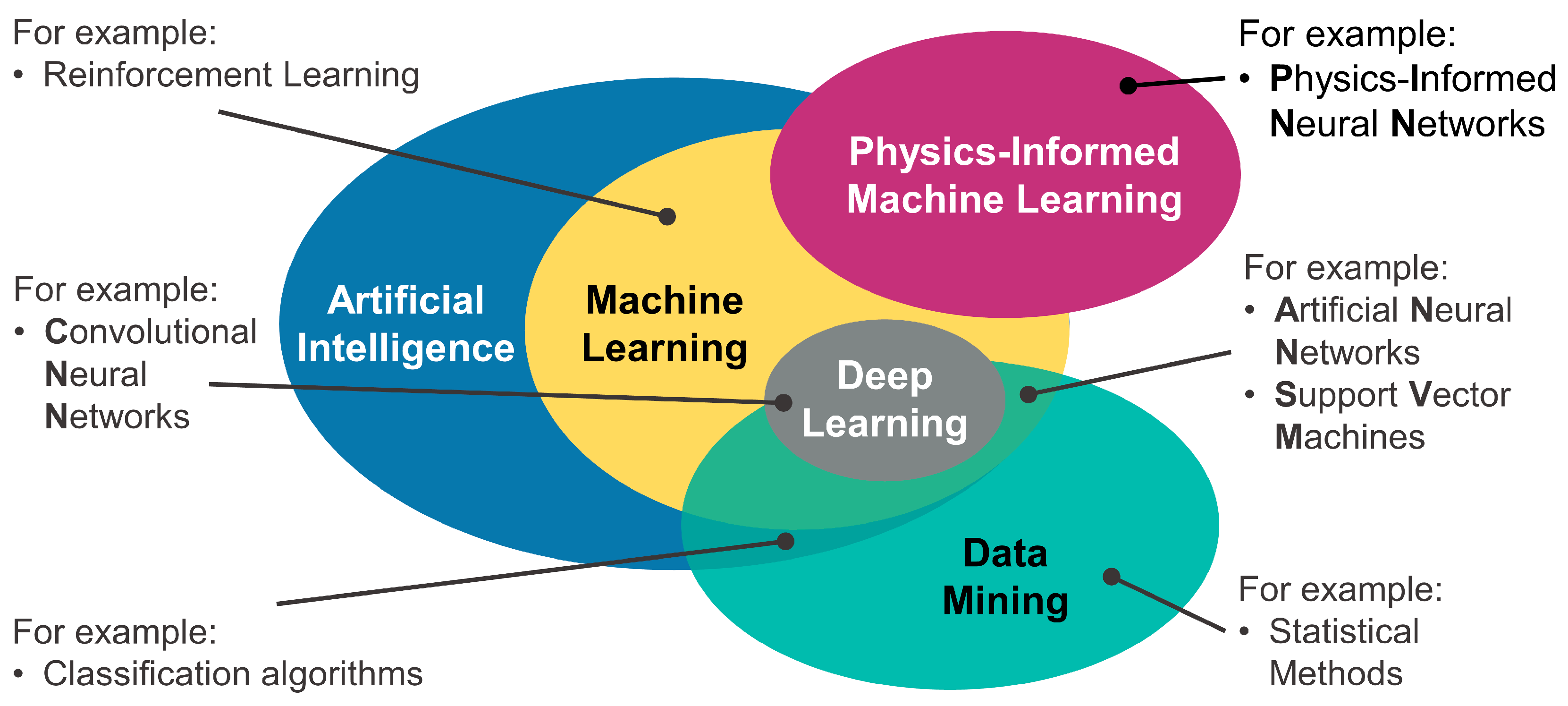
1. Artificial Intelligence and Machine Learning in Tribology
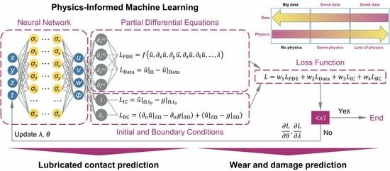
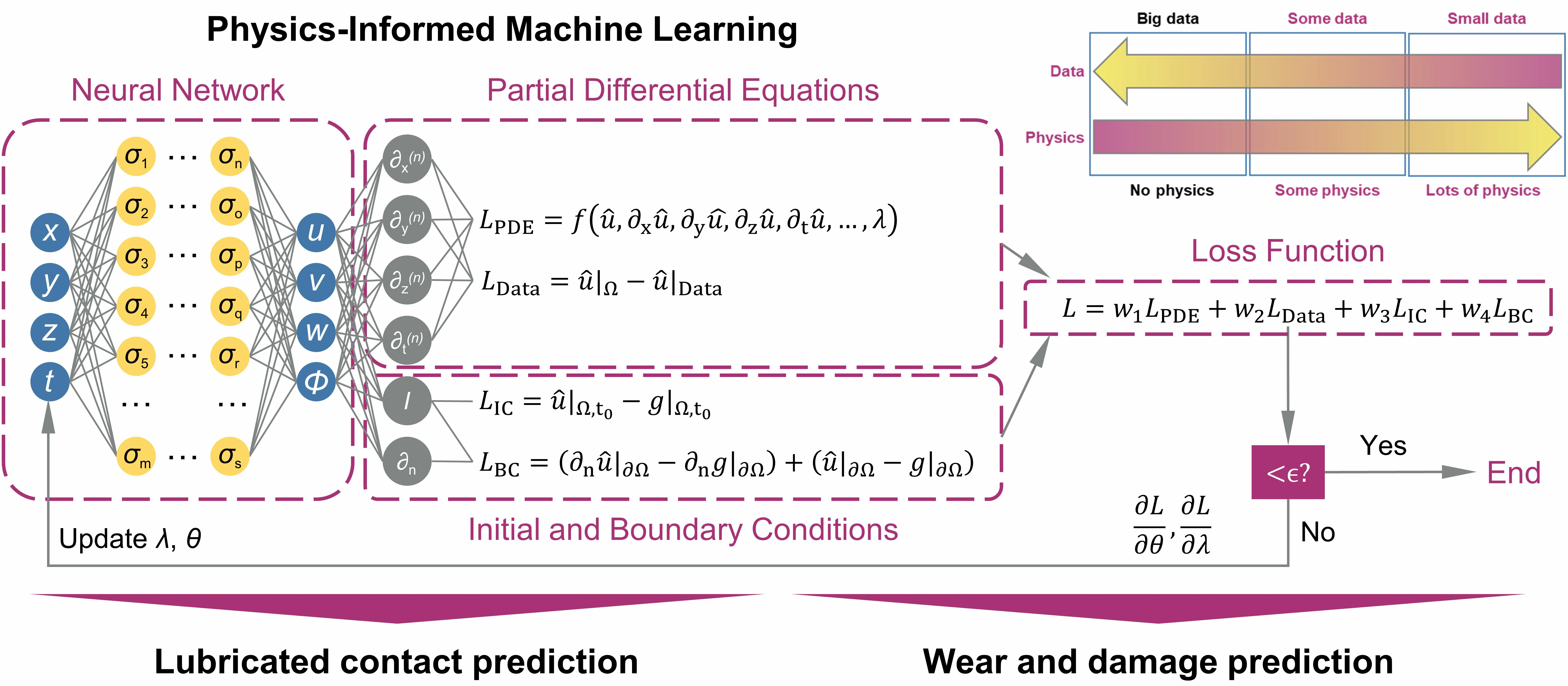
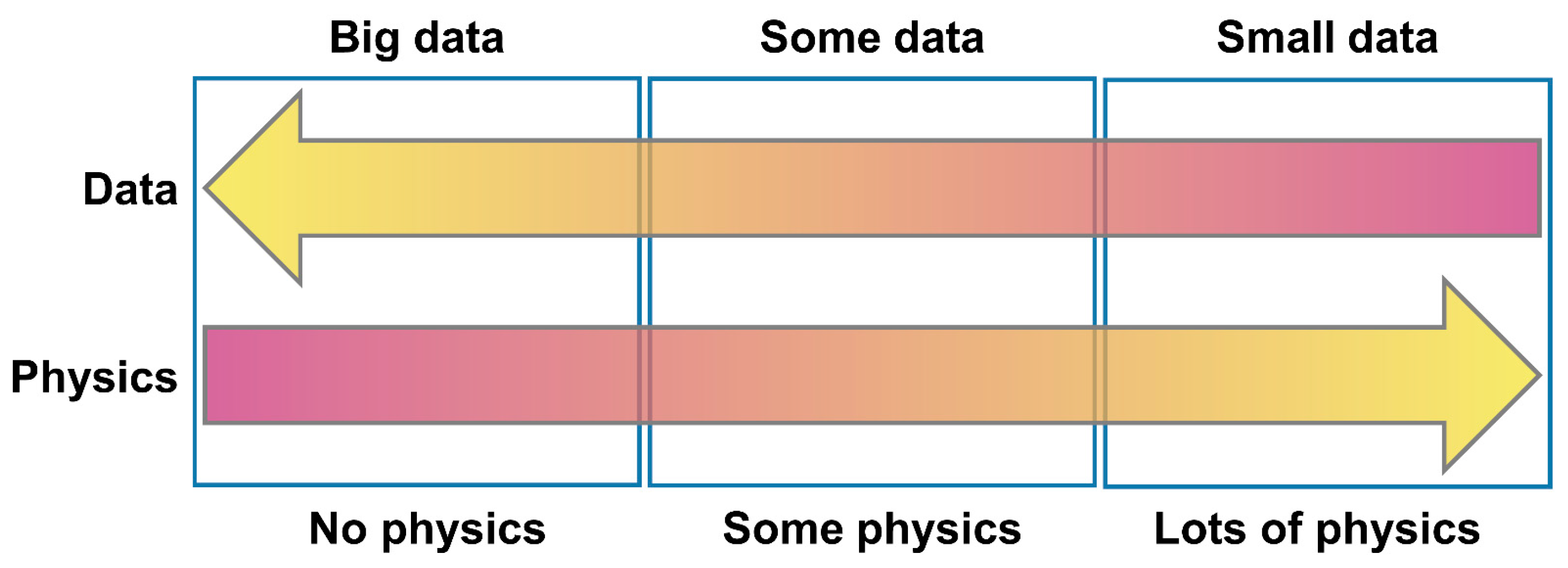
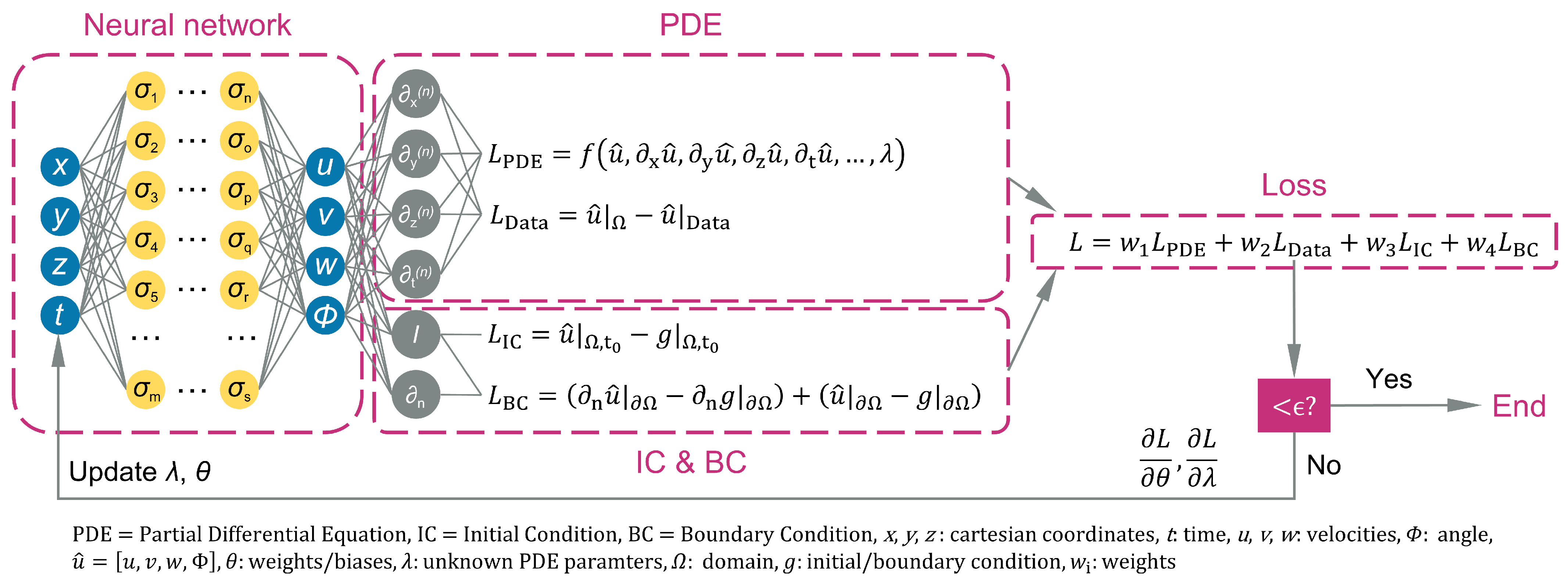
2. Physics-Informed Machine Learning
3. Physics-Informed Machine Learning in Tribology
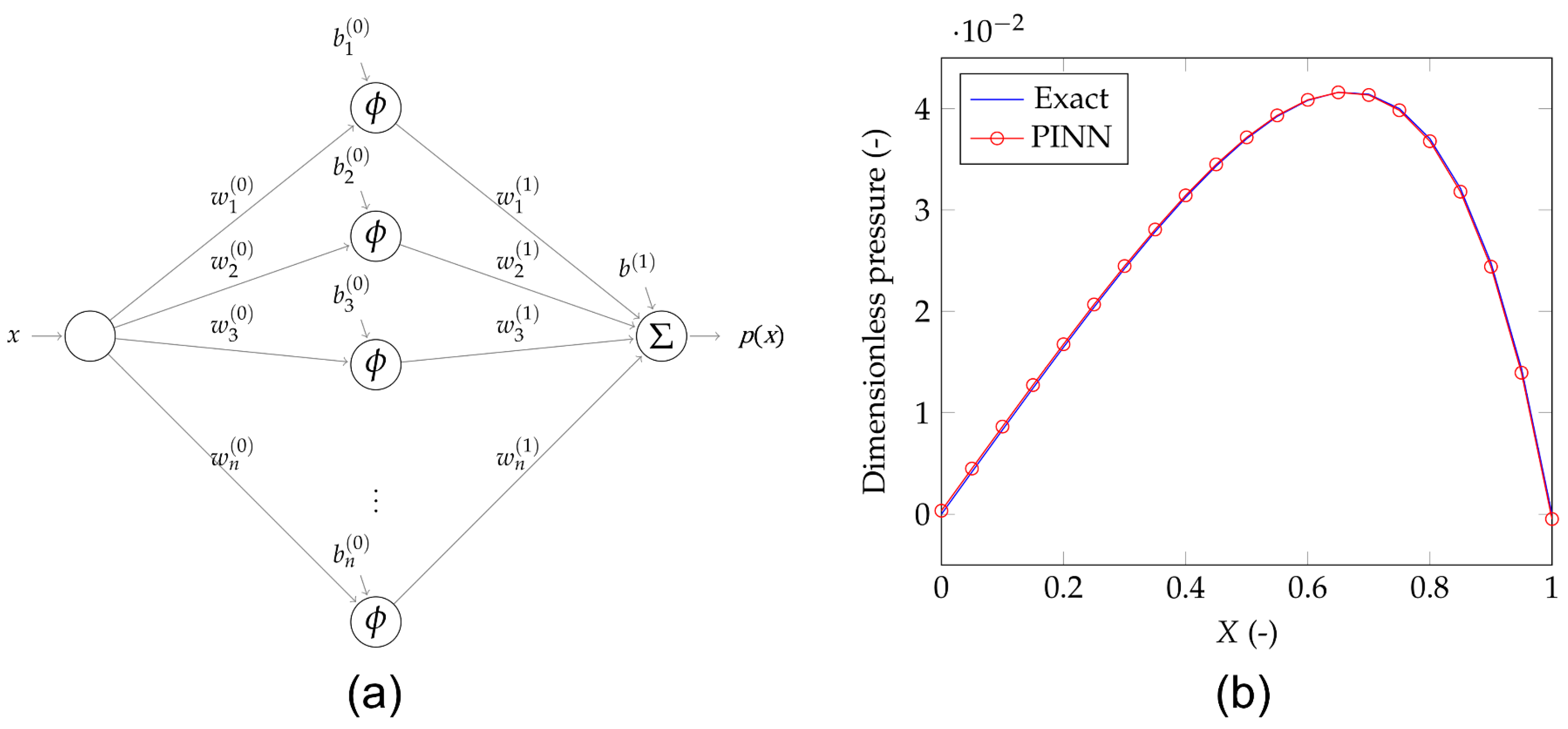
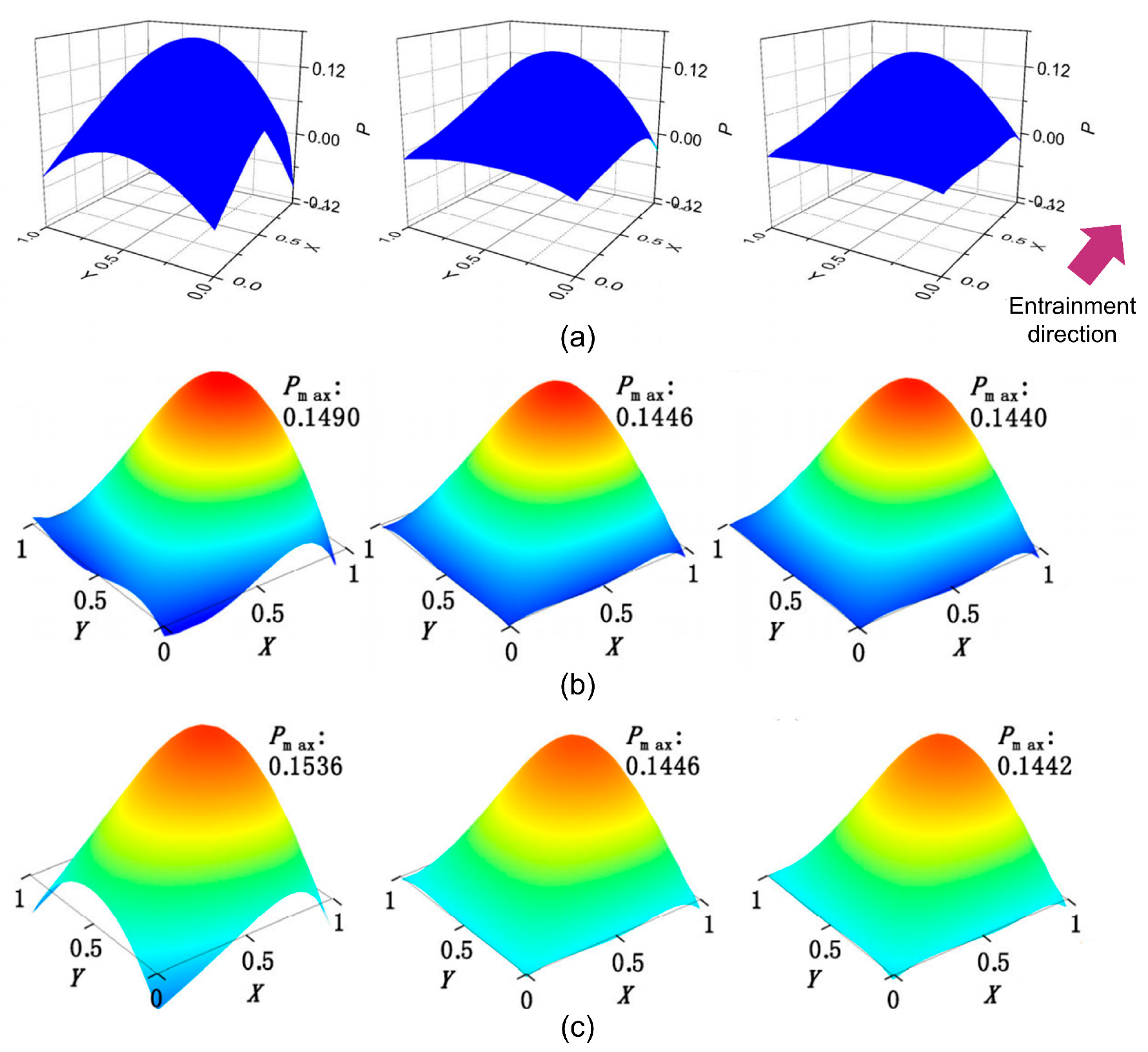
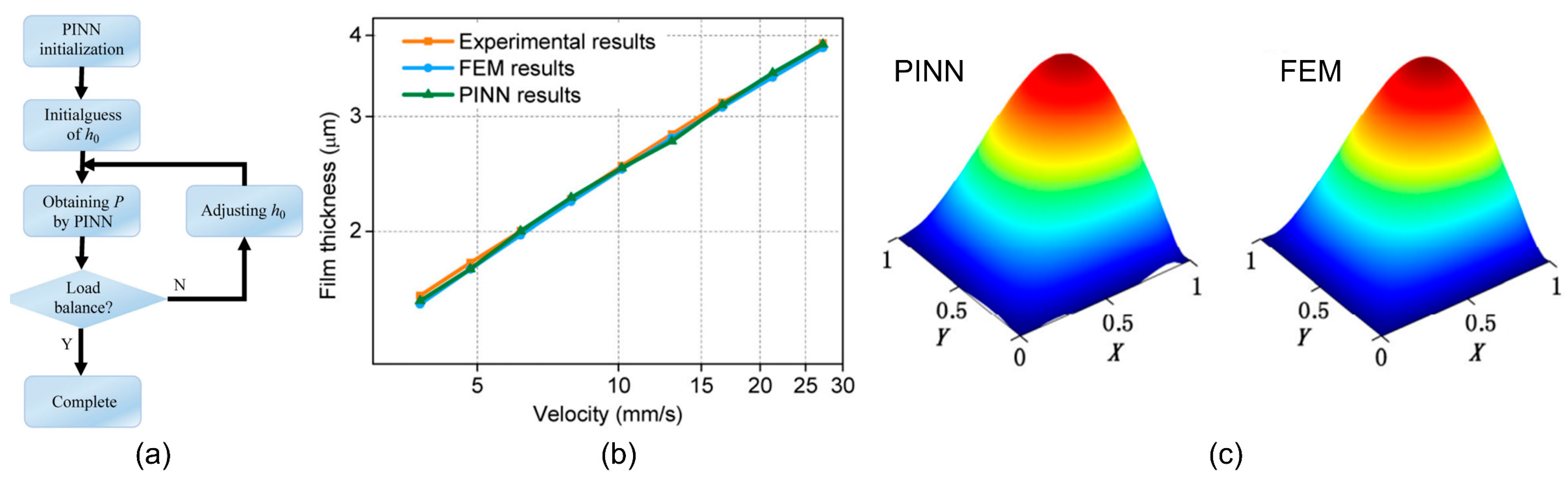
3.1. Lubrication Prediction
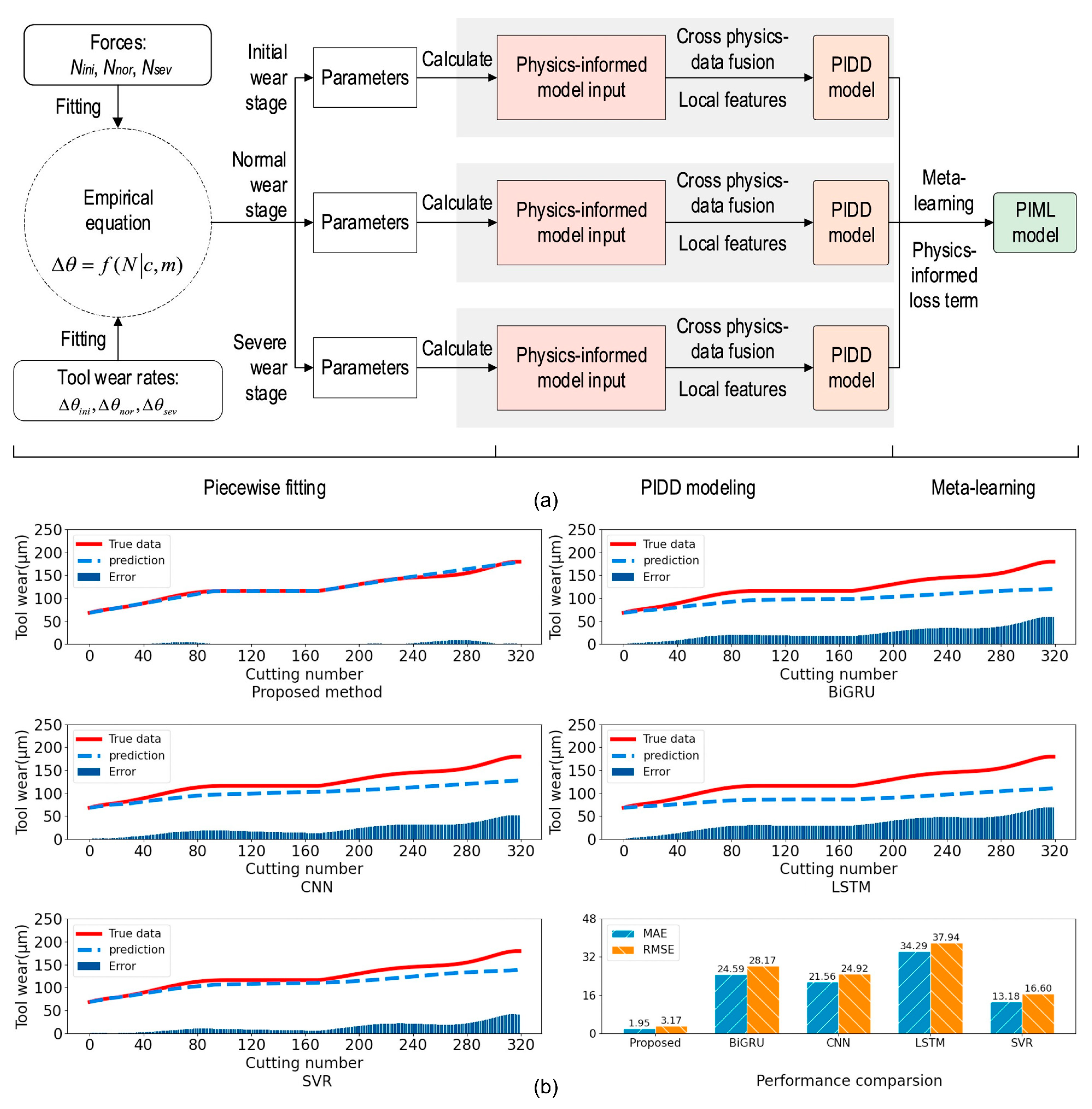
3.2. Wear and Damage Prediction
4. Concluding Remarks
Author Contributions
Funding
Data Availability Statement
Acknowledgments
Conflicts of Interest
References
- Marian, M.; Tremmel, S. Current Trends and Applications of Machine Learning in Tribology—A Review. Lubricants 2021, 9, 86. [Google Scholar] [CrossRef]
- Rosenkranz, A.; Marian, M.; Profito, F.J.; Aragon, N.; Shah, R. The Use of Artificial Intelligence in Tribology—A Perspective. Lubricants 2021, 9, 2. [Google Scholar] [CrossRef]
- Bell, J. Machine Learning: Hands-On for Developers and Technical Professionals; Wiley: Hoboken, NJ, USA, 2014; ISBN 978-1-118-88906-0. [Google Scholar]
- Breiman, L. Random Forests. Mach. Learn. 2001, 45, 5–32. [Google Scholar] [CrossRef]
- Schölkopf, B.; Smola, A.J. Learning with Kernels: Support Vector Machines, Regularization, Optimization, and Beyond; MIT Press: Cambridge, MA, USA, 2002; ISBN 978-0-262-19475-4. [Google Scholar]
- Sarkar, D.; Bali, R.; Sharma, T. Practical Machine Learning with Python: A Problem-Solver’s Guide to Building Real-World Intelligent Systems; Apress: Berkeley, CA, USA, 2017; ISBN 978-1-4842-3206-4. [Google Scholar]
- Kruse, R.; Borgelt, C.; Braune, C.; Klawonn, F.; Moewes, C.; Steinbrecher, M. Computational Intelligence: Eine Methodische Einführung in Künstliche Neuronale Netze, Evolutionäre Algorithmen, Fuzzy-Systeme und Bayes-Netze, 2nd ed.; Überarbeitete und Erweiterte Auflage; Springer Vieweg: Wiesbaden, Germany, 2015; ISBN 978-3-658-10904-2. [Google Scholar]
- Gerschütz, B.; Sauer, C.; Wallisch, A.; Mehlstäubl, J.; Kormann, A.; Schleich, B.; Alber-Laukant, B.; Paetzold, K.; Rieg, F.; Wartzack, S. Towards Customized Digital Engineering: Challenges and potentials of adapting digital engineering methods for the product development process. In Stuttgarter Symposium für Produktentwicklung SSP 2021; Fraunhofer IAO, Ed.; Fraunhofer IAO: Stuttgart, Germany, 2021; pp. 93–104. [Google Scholar]
- Kurt, H.I.; Oduncuoglu, M. Application of a Neural Network Model for Prediction of Wear Properties of Ultrahigh Molecular Weight Polyethylene Composites. Int. J. Polym. Sci. 2015, 2015, 315710. [Google Scholar] [CrossRef]
- Vinoth, A.; Datta, S. Design of the ultrahigh molecular weight polyethylene composites with multiple nanoparticles: An artificial intelligence approach. J. Compos. Mater. 2020, 54, 179–192. [Google Scholar] [CrossRef]
- Hasan, M.S.; Kordijazi, A.; Rohatgi, P.K.; Nosonovsky, M. Triboinformatics Approach for Friction and Wear Prediction of Al-Graphite Composites Using Machine Learning Methods. J. Tribol. Trans. ASME 2022, 144, 011701. [Google Scholar] [CrossRef]
- Hasan, M.S.; Kordijazi, A.; Rohatgi, P.K.; Nosonovsky, M. Triboinformatic modeling of dry friction and wear of aluminum base alloys using machine learning algorithms. Tribol. Int. 2021, 161, 107065. [Google Scholar] [CrossRef]
- Kanai, R.A.; Desavale, R.G.; Chavan, S.P. Experimental-Based Fault Diagnosis of Rolling Bearings Using Artificial Neural Network. J. Tribol. Trans. ASME 2016, 138, 031103. [Google Scholar] [CrossRef]
- Prost, J.; Cihak-Bayr, U.; Neacșu, I.A.; Grundtner, R.; Pirker, F.; Vorlaufer, G. Semi-Supervised Classification of the State of Operation in Self-Lubricating Journal Bearings Using a Random Forest Classifier. Lubricants 2021, 9, 50. [Google Scholar] [CrossRef]
- Argatov, I.; Jin, X. Time-delay neural network modeling of the running-in wear process. Tribol. Int. 2023, 178, 108021. [Google Scholar] [CrossRef]
- Marian, M.; Grützmacher, P.; Rosenkranz, A.; Tremmel, S.; Mücklich, F.; Wartzack, S. Designing surface textures for EHL point-contacts—Transient 3D simulations, meta-modeling and experimental validation. Tribol. Int. 2019, 137, 152–163. [Google Scholar] [CrossRef]
- Dai, K.; Gao, X. Estimating antiwear properties of lubricant additives using a quantitative structure tribo-ability relationship model with back propagation neural network. Wear 2013, 306, 242–247. [Google Scholar] [CrossRef]
- Bhaumik, S.; Pathak, S.D.; Dey, S.; Datta, S. Artificial intelligence based design of multiple friction modifiers dispersed castor oil and evaluating its tribological properties. Tribol. Int. 2019, 140, 105813. [Google Scholar] [CrossRef]
- Padhi, P.K.; Satapathy, A. Analysis of Sliding Wear Characteristics of BFS Filled Composites Using an Experimental Design Approach Integrated with ANN. Tribol. Trans. 2013, 56, 789–796. [Google Scholar] [CrossRef]
- Gangwar, S.; Pathak, V.K. Dry sliding wear characteristics evaluation and prediction of vacuum casted marble dust (MD) reinforced ZA-27 alloy composites using hybrid improved bat algorithm and ANN. Mater. Today Commun. 2020, 25, 101615. [Google Scholar] [CrossRef]
- Sahraoui, T.; Guessasma, S.; Fenineche, N.E.; Montavon, G.; Coddet, C. Friction and wear behaviour prediction of HVOF coatings and electroplated hard chromium using neural computation. Mater. Lett. 2004, 58, 654–660. [Google Scholar] [CrossRef]
- Boidi, G.; Rodrigues da Silva, M.; Profito, F.J.J.; Machado, I.F. Using Machine Learning Radial Basis Function (RBF) Method for Predicting Lubricated Friction on Textured and Porous Surfaces. Surf. Topogr. Metrol. Prop. 2020, 8, 044002. [Google Scholar] [CrossRef]
- Gupta, S.K.; Pandey, K.N.; Kumar, R. Artificial intelligence-based modelling and multi-objective optimization of friction stir welding of dissimilar AA5083-O and AA6063-T6 aluminium alloys. Proc. Inst. Mech. Eng. Part L J. Mater. Des. Appl. 2018, 232, 333–342. [Google Scholar] [CrossRef]
- Anand, K.; Shrivastava, R.; Tamilmannan, K.; Sathiya, P. A Comparative Study of Artificial Neural Network and Response Surface Methodology for Optimization of Friction Welding of Incoloy 800 H. Acta Metall. Sin. (Engl. Lett.) 2015, 28, 892–902. [Google Scholar] [CrossRef]
- Francisco, A.; Lavie, T.; Fatu, A.; Villechaise, B. Metamodel-Assisted Optimization of Connecting Rod Big-End Bearings. J. Tribol. Trans. ASME 2013, 135, 041704. [Google Scholar] [CrossRef]
- Zavos, A.; Katsaros, K.P.; Nikolakopoulos, P.G. Optimum Selection of Coated Piston Rings and Thrust Bearings in Mixed Lubrication for Different Lubricants Using Machine Learning. Coatings 2022, 12, 704. [Google Scholar] [CrossRef]
- Tremmel, S.; Marian, M. Machine Learning in Tribology—More than Buzzwords? Lubricants 2022, 10, 68. [Google Scholar] [CrossRef]
- Paturi, U.M.R.; Palakurthy, S.T.; Reddy, N.S. The Role of Machine Learning in Tribology: A Systematic Review. Arch Comput. Methods Eng 2023, 30, 1345–1397. [Google Scholar] [CrossRef]
- Sose, A.T.; Joshi, S.Y.; Kunche, L.K.; Wang, F.; Deshmukh, S.A. A review of recent advances and applications of machine learning in tribology. Phys. Chem. Chem. Phys. 2023, 25, 4408–4443. [Google Scholar] [CrossRef]
- Yin, N.; Xing, Z.; He, K.; Zhang, Z. Tribo-informatics approaches in tribology research: A review. Friction 2023, 11, 1–22. [Google Scholar] [CrossRef]
- Argatov, I. Artificial Neural Networks (ANNs) as a Novel Modeling Technique in Tribology. Front. Mech. Eng. 2019, 5, 1074. [Google Scholar] [CrossRef]
- Boidi, G.; Grützmacher, P.G.; Varga, M.; Da Rodrigues Silva, M.; Gachot, C.; Dini, D.; Profito, F.J.; Machado, I.F. Tribological Performance of Random Sinter Pores vs. Deterministic Laser Surface Textures: An Experimental and Machine Learning Approach. In Tribology of Machine Elements-Fundamentals and Applications; IntechOpen: London, UK, 2021. [Google Scholar] [CrossRef]
- de La Guerra Ochoa, E.; Otero, J.E.; Tanarro, E.C.; Morgado, P.L.; Lantada, A.D.; Munoz-Guijosa, J.M.; Sanz, J.M. Optimising lubricated friction coefficient by surface texturing. Proc. Inst. Mech. Eng. Part C J. Mech. Eng. Sci. 2013, 227, 2610–2619. [Google Scholar] [CrossRef]
- Gyurova, L.A.; Miniño-Justel, P.; Schlarb, A.K. Modeling the sliding wear and friction properties of polyphenylene sulfide composites using artificial neural networks. Wear 2010, 268, 708–714. [Google Scholar] [CrossRef]
- Thankachan, T.; Soorya Prakash, K.; Kamarthin, M. Optimizing the Tribological Behavior of Hybrid Copper Surface Composites Using Statistical and Machine Learning Techniques. J. Tribol. Trans. ASME 2018, 140, 031610. [Google Scholar] [CrossRef]
- Sadık Ünlü, B.; Durmuş, H.; Meriç, C. Determination of tribological properties at CuSn10 alloy journal bearings by experimental and means of artificial neural networks method. Ind Lubr. Tribol. 2012, 64, 258–264. [Google Scholar] [CrossRef]
- Senatore, A.; D’Agostino, V.; Di Giuda, R.; Petrone, V. Experimental investigation and neural network prediction of brakes and clutch material frictional behaviour considering the sliding acceleration influence. Tribol. Int. 2011, 44, 1199–1207. [Google Scholar] [CrossRef]
- Bhaumik, S.; Mathew, B.R.; Datta, S. Computational intelligence-based design of lubricant with vegetable oil blend and various nano friction modifiers. Fuel 2019, 241, 733–743. [Google Scholar] [CrossRef]
- Schwarz, S.; Grillenberger, H.; Graf-Goller, O.; Bartz, M.; Tremmel, S.; Wartzack, S. Using Machine Learning Methods for Predicting Cage Performance Criteria in an Angular Contact Ball Bearing. Lubricants 2022, 10, 25. [Google Scholar] [CrossRef]
- Marian, M.; Mursak, J.; Bartz, M.; Profito, F.J.; Rosenkranz, A.; Wartzack, S. Predicting EHL film thickness parameters by machine learning approaches. Friction 2022, 11, 992–1013. [Google Scholar] [CrossRef]
- Walker, J.; Questa, H.; Raman, A.; Ahmed, M.; Mohammadpour, M.; Bewsher, S.R.; Offner, G. Application of Tribological Artificial Neural Networks in Machine Elements. Tribol. Lett. 2023, 71, 3. [Google Scholar] [CrossRef]
- Hess, N.; Shang, L. Development of a Machine Learning Model for Elastohydrodynamic Pressure Prediction in Journal Bearings. J. Tribol. Trans. ASME 2022, 144, 081603. [Google Scholar] [CrossRef]
- Garabedian, N.T.; Schreiber, P.J.; Brandt, N.; Zschumme, P.; Blatter, I.L.; Dollmann, A.; Haug, C.; Kümmel, D.; Li, Y.; Meyer, F.; et al. Generating FAIR research data in experimental tribology. Sci. Data 2022, 9, 315. [Google Scholar] [CrossRef]
- Brandt, N.; Garabedian, N.T.; Schoof, E.; Schreiber, P.J.; Zschumme, P.; Greiner, C.; Selzer, M. Managing FAIR Tribological Data Using Kadi4Mat. Data 2022, 7, 15. [Google Scholar] [CrossRef]
- Bagov, I.; Greiner, C.; Garabedian, N. Collaborative Metadata Definition using Controlled Vocabularies, and Ontologies. RIO 2022, 8, e94931. [Google Scholar] [CrossRef]
- Kügler, P.; Marian, M.; Dorsch, R.; Schleich, B.; Wartzack, S. A Semantic Annotation Pipeline towards the Generation of Knowledge Graphs in Tribology. Lubricants 2022, 10, 18. [Google Scholar] [CrossRef]
- Kügler, P.; Marian, M.; Schleich, B.; Tremmel, S.; Wartzack, S. tribAIn—Towards an Explicit Specification of Shared Tribological Understanding. Appl. Sci. 2020, 10, 4421. [Google Scholar] [CrossRef]
- Karniadakis, G.E.; Kevrekidis, I.G.; Lu, L.; Perdikaris, P.; Wang, S.; Yang, L. Physics-informed machine learning. Nat. Rev. Phys. 2021, 3, 422–440. [Google Scholar] [CrossRef]
- Raissi, M.; Perdikaris, P.; Karniadakis, G.E. Physics-informed neural networks: A deep learning framework for solving forward and inverse problems involving nonlinear partial differential equations. J. Comput. Phys. 2019, 378, 686–707. [Google Scholar] [CrossRef]
- Raissi, M.; Karniadakis, G.E. Hidden physics models: Machine learning of nonlinear partial differential equations. J. Comput. Phys. 2018, 357, 125–141. [Google Scholar] [CrossRef]
- Lagaris, I.E.; Likas, A.; Fotiadis, D.I. Artificial neural networks for solving ordinary and partial differential equations. IEEE Trans. Neural Netw. 1998, 9, 987–1000. [Google Scholar] [CrossRef]
- Pioch, F.; Harmening, J.H.; Müller, A.M.; Peitzmann, F.-J.; Schramm, D.; el Moctar, O. Turbulence Modeling for Physics-Informed Neural Networks: Comparison of Different RANS Models for the Backward-Facing Step Flow. Fluids 2023, 8, 43. [Google Scholar] [CrossRef]
- Almajid, M.M.; Abu-Al-Saud, M.O. Prediction of porous media fluid flow using physics informed neural networks. J. Pet. Sci. Eng. 2022, 208, 109205. [Google Scholar] [CrossRef]
- Rudy, S.H.; Brunton, S.L.; Proctor, J.L.; Kutz, J.N. Data-driven discovery of partial differential equations. Sci. Adv. 2017, 3, e1602614. [Google Scholar] [CrossRef]
- Chen, D.; Li, Y.; Liu, K.; Li, Y. A physics-informed neural network approach to fatigue life prediction using small quantity of samples. Int. J. Fatigue 2023, 166, 107270. [Google Scholar] [CrossRef]
- Lee, S.; Popovics, J. Applications of physics-informed neural networks for property characterization of complex materials. RILEM Tech. Lett. 2022, 7, 178–188. [Google Scholar] [CrossRef]
- Taç, V.; Linka, K.; Sahli-Costabal, F.; Kuhl, E.; Tepole, A.B. Benchmarking physics-informed frameworks for data-driven hyperelasticity. Comput. Mech. 2023. [Google Scholar] [CrossRef]
- Pun, G.P.P.; Batra, R.; Ramprasad, R.; Mishin, Y. Physically informed artificial neural networks for atomistic modeling of materials. Nat. Commun. 2019, 10, 2339. [Google Scholar] [CrossRef] [PubMed]
- Zhang, Z.; Gu, G.X. Physics-informed deep learning for digital materials. Theor. Appl. Mech. Lett. 2021, 11, 100220. [Google Scholar] [CrossRef]
- Katsikis, D.; Muradova, A.D.; Stavroulakis, G.E. A Gentle Introduction to Physics-Informed Neural Networks, with Applications in Static Rod and Beam Problems. J. Adv. App. Comput. Math. 2022, 9, 103–128. [Google Scholar] [CrossRef]
- Moradi, S.; Duran, B.; Eftekhar Azam, S.; Mofid, M. Novel Physics-Informed Artificial Neural Network Architectures for System and Input Identification of Structural Dynamics PDEs. Buildings 2023, 13, 650. [Google Scholar] [CrossRef]
- van Herten, R.L.M.; Chiribiri, A.; Breeuwer, M.; Veta, M.; Scannell, C.M. Physics-informed neural networks for myocardial perfusion MRI quantification. Med. Image Anal. 2022, 78, 102399. [Google Scholar] [CrossRef]
- Sahli Costabal, F.; Yang, Y.; Perdikaris, P.; Hurtado, D.E.; Kuhl, E. Physics-Informed Neural Networks for Cardiac Activation Mapping. Front. Phys. 2020, 8, 42. [Google Scholar] [CrossRef]
- Almqvist, A. Fundamentals of Physics-Informed Neural Networks Applied to Solve the Reynolds Boundary Value Problem. Lubricants 2021, 9, 82. [Google Scholar] [CrossRef]
- Bach, F. Breaking the Curse of Dimensionality with Convex Neural Networks. J. Mach. Learn. Res. 2014, 18, 629–681. [Google Scholar]
- Zhao, Y.; Guo, L.; Wong, P.P.L. Application of physics-informed neural network in the analysis of hydrodynamic lubrication. Friction 2023, 11, 1253–1264. [Google Scholar] [CrossRef]
- Zubov, K.; McCarthy, Z.; Ma, Y.; Calisto, F.; Pagliarino, V.; Azeglio, S.; Bottero, L.; Luján, E.; Sulzer, V.; Bharambe, A.; et al. NeuralPDE: Automating Physics-Informed Neural Networks (PINNs) with Error Approximations. arXiv 2021, arXiv:2107.09443. [Google Scholar]
- Li, L.; Li, Y.; Du, Q.; Liu, T.; Xie, Y. ReF-nets: Physics-informed neural network for Reynolds equation of gas bearing. Comput. Methods Appl. Mech. Eng. 2022, 391, 114524. [Google Scholar] [CrossRef]
- Yadav, S.K.; Thakre, G. Solution of Lubrication Problems with Deep Neural Network. In Advances in Manufacturing Engineering; Dikshit, M.K., Soni, A., Davim, J.P., Eds.; Springer Nature Singapore: Singapore, 2023; pp. 471–477. ISBN 978-981-19-4207-5. [Google Scholar]
- Xi, Y.; Deng, J.; Li, Y. A solution for finite journal bearings by using physics-informed neural networks with both soft and hard constrains. Ind Lubr. Tribol. 2023, 75, 560–567. [Google Scholar] [CrossRef]
- Rom, M. Physics-informed neural networks for the Reynolds equation with cavitation modeling. Tribol. Int. 2023, 179, 108141. [Google Scholar] [CrossRef]
- Cheng, Y.; He, Q.; Huang, W.; Liu, Y.; Li, Y.; Li, D. HL-nets: Physics-informed neural networks for hydrodynamic lubrication with cavitation. Tribol. Int. 2023, 188, 108871. [Google Scholar] [CrossRef]
- Swift, H.W. The Stability of Lubricating Films in Journal Bearings. Minutes Proc. Inst. Civ. Eng. 1932, 233, 267–288. [Google Scholar]
- Stieber, W. Hydrodynamische Theorie des Gleitlagers. Das Schwimmlager; VDI: Berlin, Germany, 1933. [Google Scholar]
- Jakobsson, B.; Floberg, L. The Finite Journal Bearing, Considering Vaporization; Gumperts: Göteborg, Sweden, 1957. [Google Scholar]
- Olsson, K.-O. Cavitation in Dynamically Loaded Bearings; Gumperts: Göteborg, Sweden, 1965. [Google Scholar]
- Haviez, L.; Toscano, R.; El Youssef, M.; Fouvry, S.; Yantio, G.; Moreau, G. Semi-physical neural network model for fretting wear estimation. J. Intell. Fuzzy Syst. 2015, 28, 1745–1753. [Google Scholar] [CrossRef]
- Yucesan, Y.A.; Viana, F.A.C. A Physics-informed Neural Network for Wind Turbine Main Bearing Fatigue. Int. J. Progn. Health Manag. 2020, 11. [Google Scholar] [CrossRef]
- Shen, S.; Lu, H.; Sadoughi, M.; Hu, C.; Nemani, V.; Thelen, A.; Webster, K.; Darr, M.; Sidon, J.; Kenny, S. A physics-informed deep learning approach for bearing fault detection. Eng. Appl. Artif. Intell. 2021, 103, 104295. [Google Scholar] [CrossRef]
- Ni, Q.; Ji, J.C.; Halkon, B.; Feng, K.; Nandi, A.K. Physics-Informed Residual Network (PIResNet) for rolling element bearing fault diagnostics. Mech. Syst. Signal Process. 2023, 200, 110544. [Google Scholar] [CrossRef]
- Li, Y.; Wang, J.; Huang, Z.; Gao, R.X. Physics-informed meta learning for machining tool wear prediction. J. Manuf. Syst. 2022, 62, 17–27. [Google Scholar] [CrossRef]
- Marian, M.; Almqvist, A.; Rosenkranz, A.; Fillon, M. Numerical micro-texture optimization for lubricated contacts—A critical discussion. Friction 2022, 10, 1772–1809. [Google Scholar] [CrossRef]
- Shukla, K.; Jagtap, A.D.; Karniadakis, G.E. Parallel physics-informed neural networks via domain decomposition. J. Comput. Phys. 2021, 447, 110683. [Google Scholar] [CrossRef]
- Dwivedi, V.; Srinivasan, B. Physics Informed Extreme Learning Machine (PIELM)–A rapid method for the numerical solution of partial differential equations. Neurocomputing 2020, 391, 96–118. [Google Scholar] [CrossRef]
- Wu, C.; Zhu, M.; Tan, Q.; Kartha, Y.; Lu, L. A comprehensive study of non-adaptive and residual-based adaptive sampling for physics-informed neural networks. Comput. Methods Appl. Mech. Eng. 2023, 403, 115671. [Google Scholar] [CrossRef]


| Field of Application | PIML Approach | Year | Reference |
|---|---|---|---|
| Lubrication prediction | Using PINN to solve the 1D Reynolds BVP to predict the pressure distribution in a fluid-lubricated linear converging slider | 2021 | [64] |
| Using PINN to solve the 2D Reynolds equation to predict the pressure and film thickness distribution considering load balance in a fluid-lubricated linear converging slider | 2023 | [66] | |
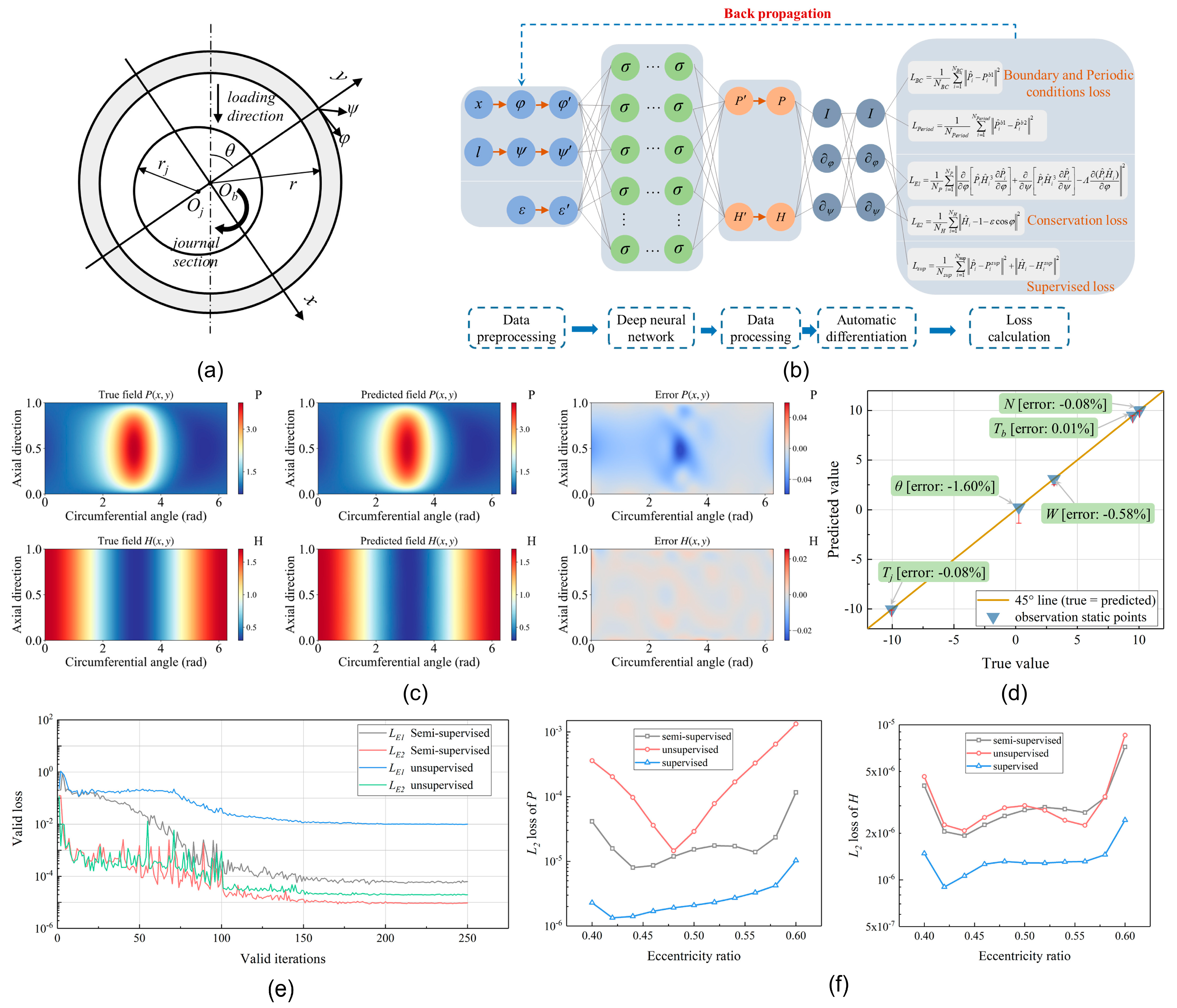
| Using supervised, semi-supervised, and unsupervised PINN to solve the 2D Reynolds equation to predict the pressure and film thickness distribution considering load balance and eccentricity in a gas-lubricated journal bearing | 2022 | [68] | |
| Using PINN to solve the 2D Reynolds equation to predict the behavior of fluid-lubricated journal as well as two-lobe bearings | 2023 | [69] | |
| Using PINN with soft and hard constraints to solve the 2D Reynolds equation to predict the pressure distribution in fluid-lubricated journal bearings at fixed eccentricity with constant and variable viscosity | 2023 | [70] | |
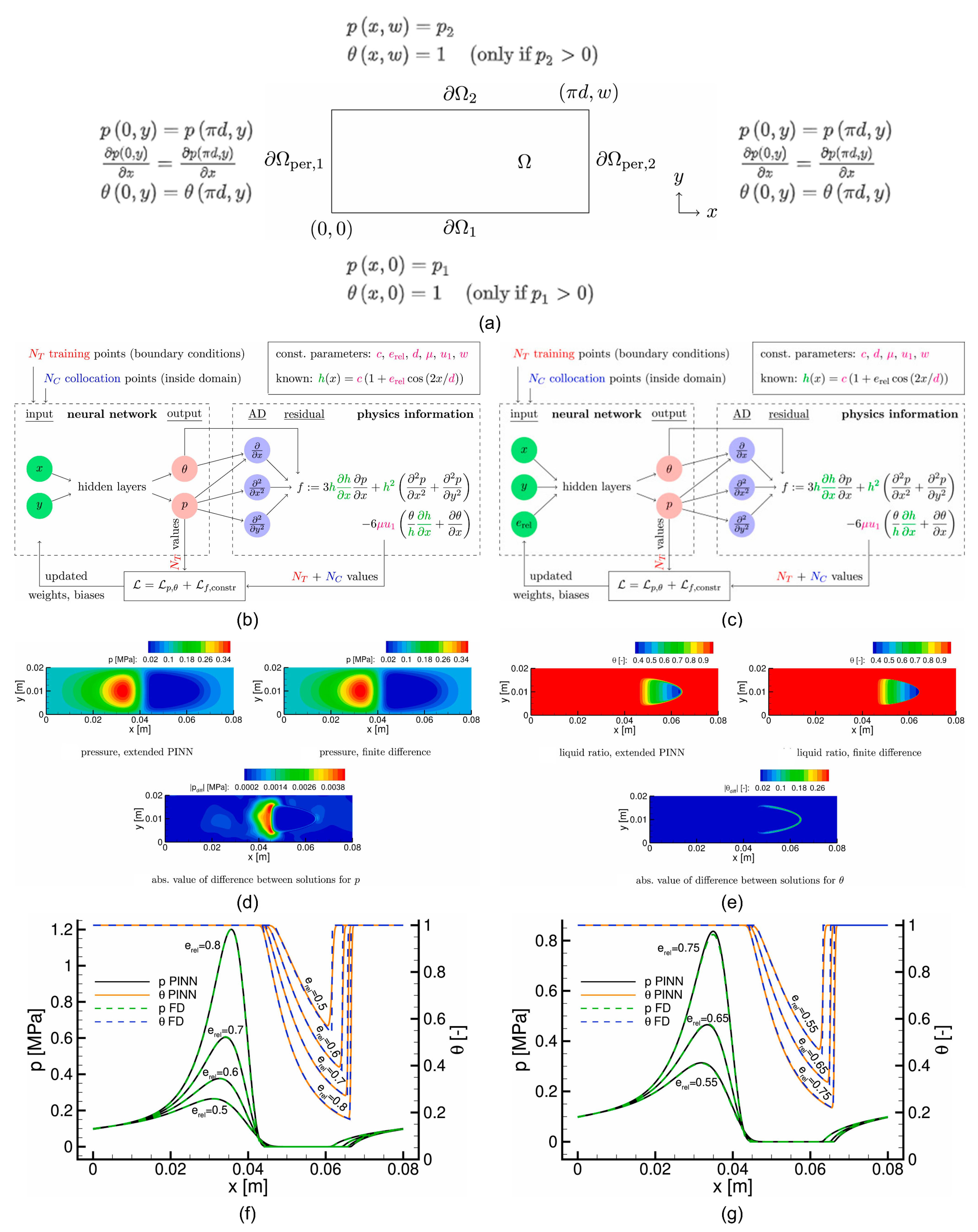
| Using PINN to solve the 2D Reynolds equation to predict the pressure and fractional film content distribution in fluid-lubricated journal bearings at fixed and variable eccentricity considering cavitation | 2023 | [71] | |
| Using PINN to solve the 2D Reynolds equation to predict the pressure and fractional film content distribution in fluid-lubricated journal bearings at fixed eccentricity considering cavitation | 2023 | [72] | |
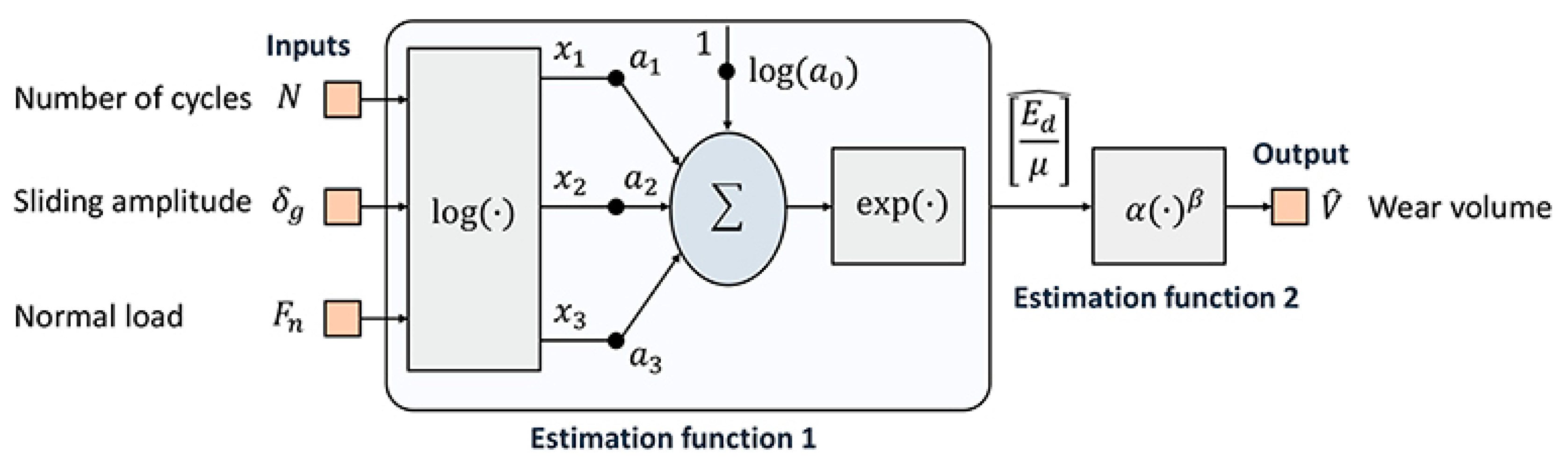
| Wear and damage prediction | Using semi PINN to find regression fitting parameters for Archard’s wear law based upon small data from fretting wear experiments | 2015 | [77] |
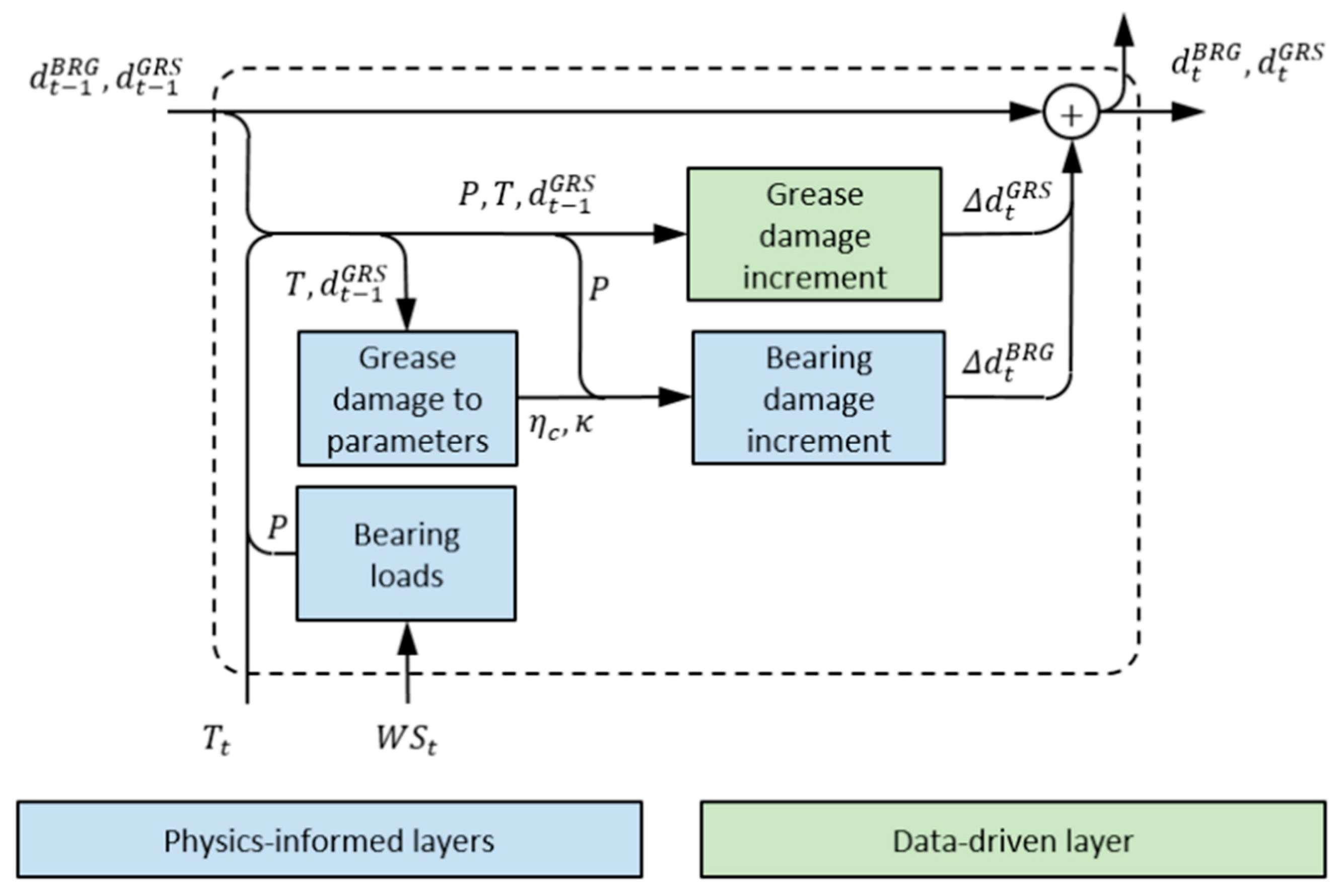
| Using hybrid PINN to predict wind turbine bearing fatigue based upon a physics-informed bearing damage model as well as data-driven grease degradation approach | 2020 | [78] | |
| Using physics-informed CNN with preceding threshold model for rolling bearing fault detection | 2021 | [79] | |
| Using physics-informed residual network for rolling bearing fault detection | 2023 | [80] | |
| Using PIML framework consisting of piecewise fitting, a hybrid physics-informed data-driven model, and meta-learning to predict tool wear | 2022 | [81] |
Disclaimer/Publisher’s Note: The statements, opinions and data contained in all publications are solely those of the individual author(s) and contributor(s) and not of MDPI and/or the editor(s). MDPI and/or the editor(s) disclaim responsibility for any injury to people or property resulting from any ideas, methods, instructions or products referred to in the content. |
© 2023 by the authors. Licensee MDPI, Basel, Switzerland. This article is an open access article distributed under the terms and conditions of the Creative Commons Attribution (CC BY) license (https://creativecommons.org/licenses/by/4.0/).
Share and Cite
Marian, M.; Tremmel, S. Physics-Informed Machine Learning—An Emerging Trend in Tribology. Lubricants 2023, 11, 463. https://doi.org/10.3390/lubricants11110463
Marian M, Tremmel S. Physics-Informed Machine Learning—An Emerging Trend in Tribology. Lubricants. 2023; 11(11):463. https://doi.org/10.3390/lubricants11110463
Chicago/Turabian StyleMarian, Max, and Stephan Tremmel. 2023. "Physics-Informed Machine Learning—An Emerging Trend in Tribology" Lubricants 11, no. 11: 463. https://doi.org/10.3390/lubricants11110463