CFD Investigation of Reynolds Flow around a Solid Obstacle

Abstract

The Reynolds equation defines the lubrication flow between the smooth contacting parts. However, it is questionable that the equation can accurately anticipate pressure behavior involving undeformed solid asperity interactions that can occur under severe operating conditions. Perhaps, the mathematical model is inaccurate and incomplete, or some HL (hydrodynamic lubrication) and EHL (elastohydrodynamic lubrication) assumptions are invalid in the mixed lubrication region. In addition, the asperity contact boundary conditions may not have been properly defined to address the issue. Such a situation motivated the recent study of a 3D CFD investigation of Reynolds flow around the solid obstacle modelled in between the converging wedge. The produced results have been compared to analytical and numerical results obtained by employing the Reynolds equation. The validated CFD simulation is compared with the identical wedge, with cylindrical asperity at the center. A significant increase in pressure has been predicted because of asperity contact. The current study shows that the mathematical formulation of the ML problem has shortcomings. This necessitates the development of a new model that can also include fluid flow around asperity contacts for the accurate prediction of generated pressure. Consequently, sustainable tribological solutions for extreme loading conditions can be devised to improve efficiency and component performance.

1. Introduction

Any manufactured surface will be rough to some degree, which can cause friction and wear on dynamically interacting surfaces under extreme loading conditions, resulting in higher maintenance and replacement costs. The micro- and nano-features on the surface are called asperities, and their sub-interactions in lubricated contact cause intense pressure that significantly reduces the fatigue life of the lubricated components [1]. Energy efficiency is crucial for businesses and society, due to limited resources and pollution issues. Various reports state that tribological contacts consume 23% of global energy [2]. For example, a piston ring and a cylinder liner pair in an IC engine is a major source of oil consumption, and works under a mixed lubrication (ML) region. This part consumes half of the fuel energy needed to overcome the frictional losses [3]. Additionally, CO₂ emissions are proportional to energy consumption. Therefore, further developments in tribological performance will reduce the economic losses caused by friction and wear, and will have a positive impact on the environment. Proper lubrication of the contacting surfaces is important to reduce power loss, and to extend the life of all mechanical components, especially the ones working under extreme loading conditions. Tribology solutions to reduce friction and wear have come a long way for decades.

In the design of lubricated engineering components, a numerical simulation of the Reynolds equation has been widely employed. Reynolds simplified the equation of hydrodynamics to define the lubrication mechanism, and established the first partial differential equation (Equation (7)) to calculate the generated pressure. According to his theory, the lubricating oil is an incompressible Newtonian fluid flowing between the smooth contacting parts, which has been referred to as Reynolds flow in this paper [4]. Dowson [5], in 1961, gave several analytical solutions and derived the Reynolds equation based on thin-film approximation (h >> L). In order to facilitate the engineering design of the mechanical components, many classical formulas for the minimum and central film thickness were developed long ago in the form of dimensionless parameters. The developed lubrication theory and analysis methods based on the Finite-Difference Method (FDM) are very imperative for designing, optimizing, and evaluating machine components such as journal bearings [5,6]. However, there are still some difficult scenarios that exist that have remained unresolved; for example, irregular surfaces in transient motion, thermal elastohydrodynamic lubrication (EHL), ultra-thin lubrication, lubricant film transition, and oil film breakdown and failure [7,8].

The full lubrication problem, for rough surfaces, with elastic deformation and viscosity fluctuation, is highly nonlinear. The conventional approach for solving the Reynolds equation is plagued with slow convergence and unwanted solution instability. A few methods have been developed to deal with the nonlinearity of the lubrication problem, which have been reviewed in reference [9]. Lubrecht [10], Venner [11], and Ai [12] have used the Multi-grid (MG) approach to improve solution accuracy and to accelerate convergence. The MG method allows the mesh to shift from coarse to fine and fine to coarse constantly, to reduce errors, as the errors decrease rapidly when the frequency of the errors and the mesh size are equal. Additionally, the discrete convolution (DC), Fast Fourier Transformation (FFT) (DC-FFT) [13], and multilevel multi-integration [14] methods have significantly ramped up the EHL numerical simulation for elastic deformation calculations [15]. In areas where the film thickness is very small (approaching zero), Zhu and Hu [16] proposed a semi-system approach, which has been further developed by many researchers. Zhu [8] introduced the Progressive Mesh Densification (PMD) method to quickly solve ultra-thin and mixed EHL problems. In the following review publications, these methodologies have been briefly outlined [9,17,18,19]. There have been several deterministic models developed in the past, but none have been applied to the typical configuration of rolling element bearings that can be found in industrial applications [20]. Dobrica and Fillon et al. [20] used the active set contact algorithm to simulate the partial journal bearing, because this method permits the film thickness to collapse to zero without imposing any limitation to the minimum film thickness. Refer to reference [20] for more information on the active set contact algorithm. Later, in 2018, Cui and Gu et al. [21] solved the transient ML problem, where the asperity contact and the hydrodynamic effect of the lubricant is calculated separately. The asperity contact pressure is calculated using the Greenwood–Williamson (GW) contact model [22], and the hydrodynamic pressure is calculated using the modified average Reynolds equation [23], using the Finite Element Method (FEM).

In recent years, CFD (Computational Fluid Dynamics) has also been popular for solving EHL problems, because in CFD users do not need to write their own codes to simulate pressure and film thickness [24,25,26,27,28,29]. However, it uses a Finite Volume Method (FVM) to directly solve the Navier–Stokes equations for complex geometry by applying boundary conditions (BC). CFD solves the momentum and continuity equations simultaneously, and enables the fluid rheology to be modified by incorporating advanced models. In CFD, the velocity is determined using the momentum equation, and iteratively revised using the pressure equation. As a result, it has been concluded that if mass continuity is the primary concern in solving the problem, then the Reynolds equation is inappropriate [30]. On the other hand, some methods exist to experimentally measure the film thickness at the contacting surfaces; for instance, capacitance, electric resistance, X-techniques, optical interferometer, and ultrasonic methods [31,32]. However, it is difficult and expensive to experimentally measure the changes in ML where the interrupted fluid film coexists with the solid contact. Therefore, the numerical method always helps with addressing the challenges. However, the common EHL formulas are not valid at the point of solid asperity contact where the film thickness approaches zero [33], because they are based on conventional theory, which is not valid for ML, and may overestimate the film thickness [34,35].

Due to competitive performance improvements over the last few decades, machines have increasingly been operated under challenging conditions. This causes the lubricant film to become thinner to achieve a low coefficient of friction and in some conditions, it fails. For these problems, deterministic models of roughness are more famous because they can predict detailed contacts and lubrication characteristics. Generally, two methods have been adopted to model the co-existence of the lubricant and the solid contact in ML: (1) solid contact pressure and fluid film pressure are calculated separately [36,37,38], and (2) both zones are treated together with the semi-system approach [16,39,40,41]. Some stochastic models have also been proposed in the past. The most well-known is the average flow model, introduced by Patir and Cheng (PC) in 1978 [42]. The PC model is further developed based on calculating the pressure and the shear flow factors, using different methods [43,44,45,46]. However, stochastic models are not very significant for studying the local breakdown of lubricant film, and subsequent failures and wear. Recently, new numerical implementations have been introduced to determine solid contact pressure in a mixed EHL solver. Hence, to define the problem of a solid contact surrounded by a lubricant, Liu et al. [33] suggested the use of lubrication–contact interface conditions (LCICs). These BC implementations are flow direction-dependent, and have been used when the film thickness is zero between the lubricated fixed wedge-bearing problem.

It is difficult to achieve convergence and accuracy when simulating lubricant film transactions (EHL to ML) and breakdown to asperity contact, since the results vary based on the differential scheme and the mesh size used [8,15,47]. Various differential schemes derived from the Taylor series expansion are frequently utilized for the discretization of the shear flow in the Reynolds equation, such as first-order backward, second-order central, and second-order backward [47]. The first-order differential scheme is preferable in dealing with ultra-thin films for the wedge term (Couette flow), which dominates in the central area of smooth EHL interfaces [47]. Zhu et al. [48] suggested using a dense mesh to reduce the numerical errors, and to accurately solve the rough surface EHL model. Zhu, in 2007, introduced the Progressive Mesh Densification (PMD) technique [8], and explained that the MG method is unsuitable for thin-film rough surfaces, by comparing the PMD method with the MG method, using the semi-system approach. Overall, the numerical simulation of a thin lubricant film with random asperity contact at the micro-level is a complex problem, and difficult to solve numerically. On the other hand, the wrong mathematical interpretation of the problem can produce different results that are far from the actual situation, which could lead to an incorrect interpretation of frictional behavior.

Simulating micro-geometric fluctuations, along with transitory effects, was the most challenging part of numerically simulating mixed lubrication. Initially, Chang (1995) developed a deterministic model while calculating the total pressure in two parts, such as the pressure from fluid film and the pressure from the asperity interactions [36]. The solid asperity contact in this model has been incorrectly depicted by assuming a solid bump with an infinite dimension in the transverse direction, which violates flow continuity. The other model presented in 2004 [49] is based on the combination of smooth hydrodynamic and solid contact involving roughness. The generated pressure was also used to calculate the subsurface stress field. Subsequently, Jiang [50] calculated the film thickness, pressure, and temperature of an EHL point contact by assuming a stationary single asperity (Ellipsoidal Bump) between the moving smooth surfaces. To resolve the issue, Zhu and Hu [16] published a new 3D deterministic model for the mixed EHL problem, in which they solved Reynolds for both the lubricated and solid asperity contact areas. In this semi-system approach, the pressure flow disappeared with zero film thickness, allowing for a shorter version of the Reynolds equation to be used, as described in reference [16]. The Reynolds equation is certainly valid if the lubricating film is thick, and if the surfaces are approximately parallel to each other. However, if the film thickness fluctuates and micro-solid asperity contact occurs, and the lubricant flows around the rigid asperity contact, the Reynolds equation’s validity is questionable. Therefore, it is crucial to check whether the assumptions used to derive the Reynolds equation are valid during the simulation of lubricated rough surfaces with asperity interactions. For very high contact pressures, such as EHL conditions, Rajagopal et al. [51] have modified the traditional Reynolds equation and included a variation of viscosity. The numerical simulation performed using the new equation shows a higher pressure than the conventional equation.

Recently, to numerically predict the local effect of mixed lubrication problem, Liu et al. [33] presented LCICs (lubrication–contact interface conditions) BC at the interface of fluid and solid interaction. He expressed the discrete form of the Reynolds equation in four flow terms (two Poiseuille flow and two Couette flow), and eliminated some (one or two) of them, assuming that no flow can penetrate the solid boundaries of a rigid block trapped in the fixed wedge bearing. The shear flow was discretized using first-order backward discretization, and various terms of the Reynolds equation were adjusted properly around the solid asperity (square blocks and cylinders) interactions.

There has been much research on the modelling of lubricated contacts, but no model has yet been developed that can effectively and efficiently solve the ML problem, because it is difficult to simulate hydrodynamic lubrication and a solid surface interaction at the same time. Only a few papers address this issue [1,8,33,39,52,53]. While all of the proposed models have utilized the Reynolds equation; however, it is still unclear whether the Reynolds equation can accurately describe flow near sub-interactions of rigid asperities in ML. A possible reason for this could be that the mathematical model is incorrect and incomplete, or that some of the HL (hydrodynamic lubrication) and EHL assumptions are inappropriate from the perspective of an ML regime. Such a situation motivated the recent study of the 3D CFD investigation of asperity contact.

In this paper, we examine whether the Reynolds equation can be utilized to explain the flow effects generated from asperity interactions occurring under mixed lubrication. In order to approximate the asperity contact, a cylindrical pillar is modelled in the fluid domain. The Reynolds equation is a simplified version of the Navier Stokes (NS) equations, and some effects that cannot be explained by the Reynolds equation can nevertheless be described with the NS equation. CFD uses the finite volume method to iteratively solve the NS equation. Hence, in the current study, a numerically (FDM) and an analytically [6] verified CFD model of simple geometry is compared with the CFD simulation of the asperity contact model.

2. Methodology

Figure 1 depicted the model used by Reynolds to explain the lubrication mechanism. The lubricant film between the contacting surface is shaped like a wedge, with the upper surface inclined at an angle, and the lower surface translating with u velocity. For 3D steady-state and incompressible flow, the NS equations are written below.

$$\mathrm{For} \text{X-Direction}\to \left(\mathrm{u}\frac{\partial \mathrm{u}}{\partial \mathrm{x}}+\mathrm{v}\frac{\partial \mathrm{u}}{\partial \mathrm{y}}+\mathrm{w}\frac{\partial \mathrm{u}}{\partial \mathrm{z}}\right)=-\frac{1}{\mathsf{\rho }}\frac{\partial \mathrm{P}}{\partial \mathrm{x}}+\frac{\mathsf{\eta }}{\mathsf{\rho }}\left(\frac{{\partial }^2\mathrm{u}}{\partial {\mathrm{x}}^2}+\frac{{\partial }^2\mathrm{u}}{\partial {\mathrm{y}}^2}+\frac{{\partial }^2\mathrm{u}}{\partial {\mathrm{z}}^2}\right)$$

(1)

$$\mathrm{For} \text{Y-Direction}\to \left(\mathrm{u}\frac{\partial \mathrm{v}}{\partial \mathrm{x}}+\mathrm{v}\frac{\partial \mathrm{v}}{\partial \mathrm{y}}+\mathrm{w}\frac{\partial \mathrm{v}}{\partial \mathrm{z}}\right)=-\frac{1}{\mathsf{\rho }}\frac{\partial \mathrm{P}}{\partial \mathrm{y}}+\frac{\mathsf{\eta }}{\mathsf{\rho }}\left(\frac{{\partial }^2\mathrm{v}}{\partial {\mathrm{x}}^2}+\frac{{\partial }^2\mathrm{v}}{\partial {\mathrm{y}}^2}+\frac{{\partial }^2\mathrm{v}}{\partial {\mathrm{z}}^2}\right)$$

(2)

$$\mathrm{For} \text{Z-Direction}\to \left(\mathrm{u}\frac{\partial \mathrm{w}}{\partial \mathrm{x}}+\mathrm{v}\frac{\partial \mathrm{w}}{\partial \mathrm{y}}+\mathrm{w}\frac{\partial \mathrm{w}}{\partial \mathrm{z}}\right)=-\frac{1}{\mathsf{\rho }}\frac{\partial \mathrm{P}}{\partial \mathrm{Z}}+\frac{\mathsf{\eta }}{\mathsf{\rho }}\left(\frac{{\partial }^2\mathrm{w}}{\partial {\mathrm{x}}^2}+\frac{{\partial }^2\mathrm{w}}{\partial {\mathrm{y}}^2}+\frac{{\partial }^2\mathrm{w}}{\partial {\mathrm{z}}^2}\right)$$

(3)

To define the flow between the converging gap, Reynolds simplified the N-S equation into three simple forms (Equations (5)–(7)), by ignoring the terms smaller in magnitude through non-dimensionalization.

$$\frac{\partial \mathrm{P}}{\partial \mathrm{x}}=\frac{\partial }{\partial \mathrm{y}}\left(\mathsf{\eta }\frac{\partial \mathrm{u}}{\partial \mathrm{y}}\right)$$

(4)

$$\frac{\partial \mathrm{P}}{\partial \mathrm{z}}=\frac{\partial }{\partial \mathrm{y}}\left(\mathsf{\eta }\frac{\partial \mathrm{w}}{\partial \mathrm{y}}\right)$$

(5)

$$\frac{\partial \mathrm{P}}{\partial \mathrm{y}}=0 \Rightarrow \mathrm{P}=\mathrm{f}\left(\mathrm{x},\mathrm{z},\mathrm{t}\right)$$

(6)

For the detailed derivation of the Reynolds equation, readers are referred to Ref. [6].

$$\frac{\partial }{\partial \mathrm{x}}\left[-\frac{{\mathsf{\rho }\mathrm{h}}^3}{12\mathsf{\eta }}\frac{\partial \mathrm{P}}{\partial \mathrm{x}}\right]+\frac{\partial }{\partial \mathrm{z}}\left[-\frac{{\mathsf{\rho }\mathrm{h}}^3}{12\mathsf{\eta }}\frac{\partial \mathrm{P}}{\partial \mathrm{z}}\right]+\frac{\partial }{\partial \mathrm{x}}\left(\frac{\mathsf{\rho }\mathrm{h}({\mathrm{u}}_{\mathrm{h}}+{\mathrm{u}}_{0)}}{2}\right)+\frac{\partial }{\partial \mathrm{z}}\left(\frac{\mathsf{\rho }\mathrm{h}({\mathrm{w}}_{\mathrm{h}}+{\mathrm{w}}_{0)}}{2}\right)+\mathsf{\rho }\left({\mathrm{v}}_{\mathrm{h}}-{\mathrm{v}}_0\right)-{\mathsf{\rho }\mathrm{u}}_{\mathrm{h}}\frac{\partial \mathrm{h}}{\partial \mathrm{x}}-{\mathsf{\rho }\mathrm{w}}_{\mathrm{h}}\frac{\partial \mathrm{h}}{\partial \mathrm{z}}+ \mathrm{h}\frac{\partial \mathsf{\rho }}{\partial \mathrm{h}}=0$$

(7)

The developed Reynolds equation (Equation (7)) is a nonlinear equation that cannot be solved analytically. Initially, for simplicity, the Reynolds equation has been solved in one dimension (1D) to calculate dimensionless pressure. The equation is discussed in Section 3.1. This equation has been utilized to analytically calculate the 1D pressure generated in the simple wedge film thickness used in this paper.

To determine pressure for a two-dimensional (2D) lubrication problem, the simple wedge film thickness has been solved simultaneously with the Reynolds equation, which requires advanced numerical methods. Additionally, any negative pressure during the calculation has been treated as zero to avoid cavitation. By using multilevel methods, Lubrecht [10] and Venner [11] described an efficient algorithm for solving the 2D Reynolds equation that gives a more accurate and convergent solution in less time. Hence, in step two, a numerical simulation is used for the calculation of pressure, by utilizing the Finite Difference Method (FDM), and the Multigrid (MG) technique.

The CFD approach is implemented in step three, where the equations of momentum (Equations (1)–(3)) and continuity are numerically solved through the Finite Volume Method (FVM). The momentum equation is used to calculate the velocity vectors, and further iteratively corrected using the pressure equation, to ensure that continuity is satisfied in every control volume, which is the major drawback of the Reynolds equation when it is used for ML simulation.

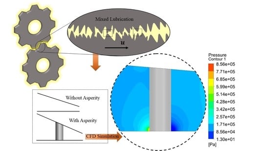
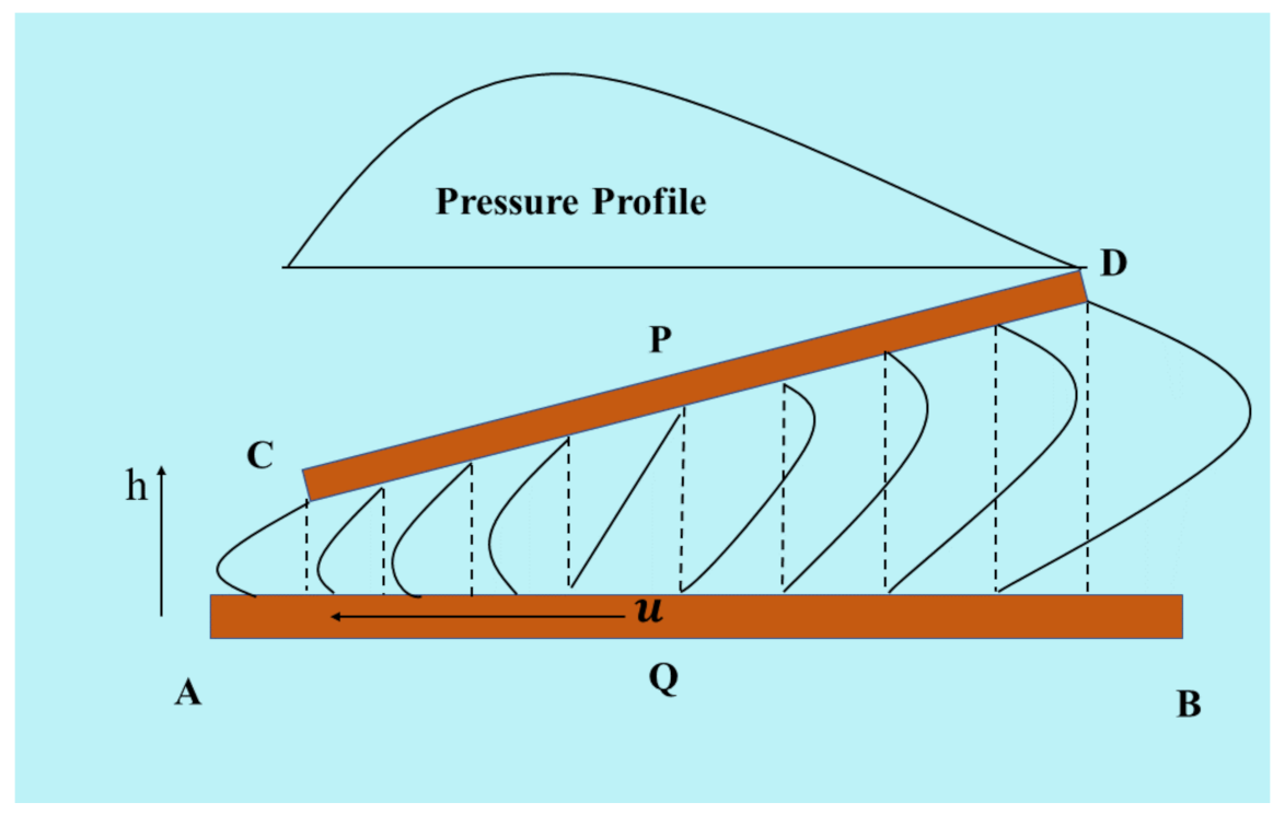
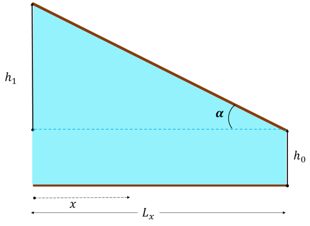
3. Simple Wedge (Without-Asperity Contact Model)

Many components work under mixed lubrication regions, such as gear, cam and followers, rolling element bearings, etc. These machine equipment generally work in minimum film thickness or boundary region during start-up and shutdown. The contacting area starts with a converging wedge-shaped gap, which generates a pressurized fluid film due to the relative movement between the contacting surfaces. This converging gap can be easily seen in conformal (journal bearing) or non-conformal (ball and roller bearing, cams and gears) lubricated contacts. Therefore, to simplify the study, a basic model of the converging gap has been used in this paper. In this work, the Reynolds number is low ($1-{10}^3$), to ensure that the convective terms are small, so that they can be ignored, like the Reynolds assumptions. The following section outlines an analytical method for calculating the pressure in converging gaps.

3.1. Analytical Method

As part of the analytical modelling, the Reynolds equation is used to calculate the pressure in one dimension. Figure 2 shows a fixed inclined slider (pad) bearing consisting of an oil film separating two nonparallel smooth surfaces, where one surface is stationary and the other is moving uniformly, forming a physical wedge. The converging wedge acts as a pressure generation mechanism to support the external load. The laminar flow of the lubricant is gravity-free, incompressible, and isothermal. The steady-state solution is derived by Hamrock [6] by assuming that the lubricant is a Newtonian fluid with constant viscosity and flow, with no-slip boundary conditions between the solid contact. The oil film thickness can be expressed as:

$${\mathrm{h}}_{\mathrm{x}}={\mathrm{h}}_0+{\mathrm{h}}_1\left(1-\frac{\mathrm{x}}{{\mathrm{L}}_{\mathrm{x}}}\right).$$

(8)

Dimensionless film thickness:

$$\overline{\mathrm{H}}={\overline{\mathrm{H}}}_0+1-\overline{\mathrm{X}}$$

(9)

To numerically calculate the pressure in one dimension, the Reynolds equation in its reduced form has been utilized:

$$\frac{\partial }{\partial \mathrm{x}}\left[-\frac{{\mathrm{h}}_{\mathrm{x}}{}^3}{12\mathsf{\eta }}\frac{\partial \mathrm{P}}{\partial \mathrm{x}}\right]=\frac{{\mathrm{u}}_0}{2}\frac{\partial {\mathrm{h}}_{\mathrm{x}}}{\partial \mathrm{x}}$$

(10)

$$\frac{\mathrm{dP}}{\mathrm{dx}}=6\mathrm{u}\left(\frac{\mathrm{h}-{\mathrm{h}}_{\mathrm{m}}}{{\mathrm{h}}^3}\right)$$

(11)

where ${\mathrm{h}}_{\mathrm{m}}$ is the film thickness when $\raisebox{1ex}{$\mathrm{dP}$}\!\left/ \!\raisebox{-1ex}{$\mathrm{dx}$}\right.=0$

Dimensionless form of the Reynolds equation:

$$\overline{\mathrm{H}}=\frac{{\mathrm{h}}_{\mathrm{x}}}{{\mathrm{h}}_1}\hspace{1em}\hspace{1em}\hspace{1em}\hspace{1em}{\overline{\mathrm{H}}}_0=\frac{{\mathrm{h}}_0}{{\mathrm{h}}_1}\hspace{1em}\hspace{1em}\overline{\mathrm{X}}=\frac{\mathrm{x}}{{\mathrm{L}}_{\mathrm{x}}}\hspace{1em}\hspace{1em}\overline{\mathrm{P}}=\frac{{\mathrm{Ph}}_1^2}{{\mathsf{\eta }\mathrm{u}}_0{\mathrm{L}}_{\mathrm{x}}}\hspace{1em}\hspace{1em}{\overline{\mathrm{H}}}_{\mathrm{m}}=\frac{{\mathrm{h}}_{\mathrm{m}}}{{\mathrm{h}}_1}$$

$$\frac{\partial \mathrm{P}}{\partial \overline{\mathrm{X}}}=6\left(\frac{\overline{\mathrm{H}}-{\overline{\mathrm{H}}}_{\mathrm{m}}}{{\overline{\mathrm{H}}}^3}\right)$$

(12)

$$\frac{\mathrm{dP}}{\mathrm{dx}}=6\mathrm{u}\left(\frac{\mathrm{h}-{\mathrm{h}}_{\mathrm{m}}}{{\mathrm{h}}^3}\right)$$

(13)

The above Equation (13) can be used to deduce to a dimensionless pressure equation by using a zero pressure boundary condition at the inlet and outlet boundaries:

$$\overline{\mathrm{P}}=\frac{6\overline{\mathrm{X}}\left(1-\overline{\mathrm{X}}\right)}{{\left({\overline{\mathrm{H}}}_0+1-\overline{\mathrm{X}}\right)}^2\left(1+2{\overline{\mathrm{H}}}_0\right)}$$

(14)

The above analytically derived pressure Equation (14) has been used to plot (shown in Figure 3) the pressure for a 0.2 mm-long simple converging wedge where the inlet height and outlet height are 0.02 mm and 0.003 mm, respectively, which gives $ℇ=0.085$. The following section describes the numerical solution of the three-dimensional lubrication problem.

3.2. Numerical Method

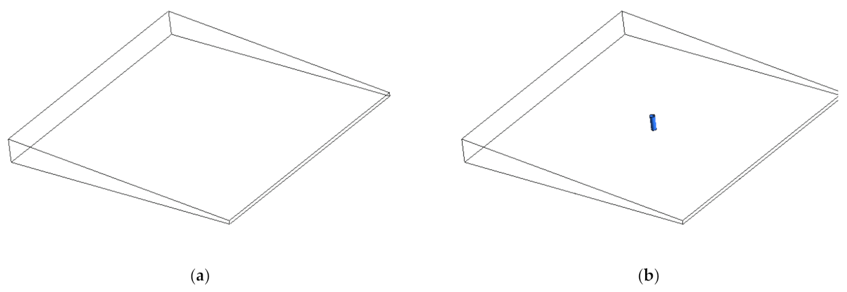
The Finite Difference Method (FDM) is widely used to solve the lubrication problem through the Reynolds equation. Initially, the partial differential equation should first be transformed into a non-dimensionless form by defining the parameters in a universal form, followed by dividing the solution region into a mesh, using a uniform or non-uniform grid. For this work, the full multigrid method has been used to obtain fast convergence.

The numerical implementations for the three-dimensional converging wedge (fixed inclined pad bearing) problem have been solved using the two-dimensional Reynolds equation shown below.

$$\frac{\partial }{\partial \mathrm{x}}\left[{\mathrm{h}}^3\frac{\partial \mathrm{P}}{\partial \mathrm{x}}\right]+\frac{\partial }{\partial \mathrm{z}}\left[{\mathrm{h}}^3\frac{\partial \mathrm{P}}{\partial \mathrm{z}}\right]=6\mathsf{\mu }\mathrm{u}\frac{\partial \mathrm{h}}{\partial \mathrm{x}}$$

(15)

Dimensionless form:

$$\overline{\mathrm{H}}=\frac{\mathrm{h}}{\mathrm{c}}\hspace{1em}\hspace{1em}\hspace{1em}\hspace{1em}\overline{\mathrm{X}}=\frac{\mathrm{x}}{{\mathrm{L}}_{\mathrm{x}}}\hspace{1em}\hspace{1em}\hspace{1em}\hspace{1em}\overline{\mathrm{Z}}=\frac{\mathrm{z}}{{\mathrm{L}}_{\mathrm{z}}}\hspace{1em}\hspace{1em}\hspace{1em}\hspace{1em}\overline{\mathrm{P}}=\frac{\mathrm{P}}{\left(\frac{{\mathrm{L}}_{\mathrm{x}}6{\mathsf{\eta }\mathrm{u}}_0}{{\mathrm{c}}^2}\right)}$$

$$\frac{\partial }{\partial \overline{\mathrm{X}}}\left[{\overline{\mathrm{H}}}^3\frac{\partial \overline{\mathrm{P}}}{\partial \overline{\mathrm{X}}}\right]+\frac{{\mathrm{L}}_{\mathrm{x}}{}^2}{{\mathrm{L}}_{\mathrm{z}}{}^2}\frac{\partial }{\partial \overline{\mathrm{Z}}}\left[{\overline{\mathrm{H}}}^3\frac{\partial \overline{\mathrm{P}}}{\partial \overline{\mathrm{Z}}}\right]=\frac{\partial \overline{\mathrm{H}}}{\partial \overline{\mathrm{X}}}$$

(16)

The 3D problem uses the X-axis to represent the direction of flow, the Z-axis is lateral to the flow direction, and the Y-axis represents the film thickness. The discretized form of the Reynolds equation has been shown in Equation(16), which uses the second-order central discretization scheme for pressure and shear flow. The solution domain is defined as $\overline{\mathrm{X}}\in \left[0,1\right], \mathrm{Z}\in \left[0,1\right]$, with zero pressure at the boundaries (${\mathrm{P}}_{\mathrm{i},\mathrm{j}}=0)$. The $\mathrm{K}={\mathrm{L}}_{\mathrm{x}}/{\mathrm{L}}_{\mathrm{z}}$ ratio is 0.1, to avoid the lateral boundaries effects on the maximum pressure calculation, by assuming that the lateral boundaries are very far from the area of study. The film thickness coefficient $\mathsf{\xi }={\overline{\mathrm{H}}}^3$, where $\overline{\mathrm{H}}$ has been defined using Equation (10). All border nodes have zero pressure, and any negative pressure is assumed to zero in this study, to avoid cavitation. For the known film thickness profiles, the pressure has been calculated using the Reynolds equation.

$$\begin{array}{l}\frac{{\mathsf{\xi }}_{\mathrm{i}+0.5,\mathrm{j}}{\overline{\mathrm{P}}}_{\mathrm{i}+1,\mathrm{j}}-\left({\mathsf{\xi }}_{\mathrm{i}+0.5,\mathrm{j}}+{\mathsf{\xi }}_{\mathrm{i}-0.5,\mathrm{j}}\right){\overline{\mathrm{P}}}_{\mathrm{i},\mathrm{j}}+{\mathsf{\xi }}_{\mathrm{i}-0.5,\mathrm{j}}{\overline{\mathrm{P}}}_{\mathrm{i}-1,\mathrm{j}}}{\Delta {\mathrm{X}}^2}\\ \hspace{1em}\hspace{1em}\hspace{1em}\hspace{1em}+{\mathrm{K}}^2\frac{{\mathsf{\xi }}_{\mathrm{i},\mathrm{j}+0.5}{\overline{\mathrm{P}}}_{\mathrm{i},\mathrm{j}+1}-\left({\mathsf{\xi }}_{\mathrm{i},\mathrm{j}+0.5}+{\mathsf{\xi }}_{\mathrm{i},\mathrm{j}-0.5}\right){\overline{\mathrm{P}}}_{\mathrm{i},\mathrm{j}}+{\mathsf{\xi }}_{\mathrm{i},\mathrm{j}-0.5}{\overline{\mathrm{P}}}_{\mathrm{i},\mathrm{j}-1}}{\Delta {\mathrm{Z}}^2}\\ \hspace{1em}\hspace{1em}\hspace{1em}\hspace{1em}=\frac{{\overline{\mathrm{H}}}_{\mathrm{i}+1,\mathrm{j}}-{\overline{\mathrm{H}}}_{\mathrm{i}-1,\mathrm{j}}}{2\Delta \mathrm{X}}\end{array}$$

(17)

The equation was solved using the multigrid method, and readers are directed to reference [11] for further details on the solution procedure.

3.3. CFD Model

CFD is famous for solving numerical simulations for very complex flow problems. In the present study, a 3D CFD model is created, using FLUENT (2021R2 package), to study the behavior of an inclined pad lubricated bearing, in configurations both with asperity and without asperity (simple wedge), considering the Newtonian flow of a lubricant. Below,

Table 1. The operating conditions and working parameters used in CFD simulation.

Parameters	Value	Unit
Velocity	1	m/s
Wedge inlet	0.02	10−3 m
Wedge outlet	0.003	10−3 m
Solid Properties
Solid Elastic Modulus, E	210	G Pa
Solid Poisson’s ratio, $\mathsf{\upsilon }$	0.3	-
Solid Density, $\mathsf{\rho }$	7850	kg/m3
Lubricant Properties
Inlet viscosity of the lubricant, $\mathsf{\eta }$	0.085	Pa·s
Kinematic viscosity, $\mathsf{\nu }$	100	mm2/s
Reynolds Number, Re	0.1	-
Oil Density	850	kg/m3
Vapor density	0.0288	kg/m3
Vapor viscosity	8.97 × 10−6	Pa·s

shows the various parameters used for the CFD simulation. The produced results without the asperity model are compared with the results produced by the cylindrical asperity contact model. The CFD results obtained from the 3D model without asperity (simple wedge) are shown in Figure 3, which shows a good agreement with the analytical and numerical results obtained by solving the Reynolds equation using the MG methods.

Model Setup

The 3D model of decreasing film thickness has been created by using a design module in the commercial software ANSYS. The surfaces of the upper and lower plates are assumed to be smooth, with a no-slip solid boundary wall. The literature shows that the quadrilateral mesh (structured) type is always recommended over the triangular mesh (unstructured) for better stability, accuracy, and convergence in the CFD simulation [28]. Thus, a quadrilateral type of mesh is used in this CFD model, and the mesh is generated using ICEM CFD software.

The CFD solver employs the double-precision, pressure-based, laminar model and the SIMPLE method to solve the momentum and continuity equations. The spatial discretization methods for the gradient, pressure, momentum, and volume fraction calculations are least-squares cell-based, PRESTO, second-order upwind, and first-order upwind, respectively. Solution initialization is performed with the hybrid initialization method that will solve the Euler equation. Further, the calculation is run for 1000 iterations for the convergence of 1 × 10⁻⁷ for continuity, and X, Y, and Z velocity and for the vapor volume fraction, respectively. It has been noticed that the residuals converged under 600 iterations. The pressure inlet and pressure outlet boundary conditions are used for the simulation setup. A multiphase model has been used to incorporate the cavitation phenomena with 13 Pa vapor pressure of lubricant oil.

3.4. Model Verification

The pressure has been compared along the centerline, at Z = 0. The pressure profile generated from the CFD model of the without-asperity case (simple wedge) is compared with the analytical results (Section 3.1) and with the multigrid method solution (Section 3.2). It was determined that the CFD pressure prediction agrees well with those predicted using analytical and numerical methods, and could be used in a further comparison of the results produced from the asperity-contact CFD model.

4. Cylindrical Asperity Contact (With Asperity Contact Model)

A simplified model of mixed lubrication is created by modelling an asperity of cylindrical shape inside a fixed wedge bearing, which has a diameter of $4 \mathsf{\mu }\mathrm{m}$, with its center at (100,0,0), as shown in Figure 4. The cylindrical asperity can be considered as an approximation of the sub-interactions of solid asperities surrounded by the lubricant. The bearing borders consist of an inlet and an outlet (at a distance of $200 \mathsf{\mu }\mathrm{m}$), which are kept at zero pressure, and the other two side borders are solid walls and are kept $200 \mathsf{\mu }\mathrm{m}$ apart. The results have been taken at the center and at near-cylindrical asperity, to investigate the influence of asperity interaction in mixed lubrication. The model is based on the assumption that the generated pressure is small in comparison to the external load, which allows the asperity to contact the lower surface. The CFD approach has been used, as described in Section 3.3. The details of the working parameters have been illustrated in Table 1. The converging wedge with the cylindrical asperity model is termed the with-asperity contact model, and is compared with the without-asperity contact model explained in Section 3.3. The 3D figure (Figure 4) depicts a comparative model of without and with asperity contact models.

The with-cylindrical asperity case has complex geometry that should be meshed carefully near solid interaction. The meshing used in this model has been shown in Figure 5. Very fine meshing has been used near asperity contact, to capture the flow properties accurately. The mesh sensitivity analysis (shown in Figure 6) has been performed to decide the optimized mesh size for the problem.

5. Results and Discussion

5.1. Pressure Comparison

The comparison of fluid pressure for the with- and without-asperity contact models have been shown together in Figure 7, along the centerline at Z = 0 and Y = 0.5 $\mathsf{\mu }\mathrm{m}$. The blue line is for the without-asperity contact CFD solution, and the red line with the rectangle is for the CFD simulation of the with-cylindrical asperity contact model. There is a significant difference in pressure between the input and the solid cylindrical asperity; similarly, behind the asperity, the pressure has reduced. To validate the results, the without-asperity contact model is compared with the numerical and analytical results produced in Section 3.1 and Section 3.2, shown in Figure 3. One can clearly see the effect of a rigid asperity contact working under mixed lubrication conditions. The reason for this higher pressure right in front of the cylindrical asperity has been further investigated by quantitatively measuring the NS equation (Section 5.3), with each term being shown in Equations (1)–(3). The following section shows the velocity comparison.

5.2. Velocity Comparison

The contour plot for velocity is presented in Figure 8, which shows discrepancies near asperity, when compared with a simple wedge (without asperity contact) 3D CFD model. Figure 9 compares the X component of velocity (u) using the contour plot. The velocity profile has also been compared in four different places on the symmetric plane. The compared velocity profiles (shown in Figure 10) are at $\mathrm{x}=50 \mathsf{\mu }\mathrm{m}$ distance from the inlet, $\mathrm{x}=96 \mathsf{\mu }\mathrm{m}$, which is right in front of the cylinder, $\mathrm{x}=104 \mathsf{\mu }\mathrm{m}$, behind the cylinder, and at $\mathrm{x}=180 \mathsf{\mu }\mathrm{m}$, near the exit, respectively. These comparisons show that away from the cylindrical asperity, the velocity profiles exactly confirm each other; hence, we can say that everything is exactly like the Reynolds theory. However, near cylindrical asperity, we have discrepancies where the velocity profile has changed.

In Figure 11, the with- and without-asperity contact models are compared on the symmetric plane for the velocity vectors colored by the velocity magnitude. The maximum and minimum velocities are the same for both models; however, near cylindrical asperity, the velocity vectors change direction on the symmetric plane, which significantly increases the vertical component of the velocity (v). It is clearly seen in Figure 11 that near cylindrical asperity, the velocity vectors are moving upward on the symmetric plane, which can illustrate the drastic rise in pressure resulting from an asperity contact. The lubricant flowing through the cylindrical asperity bifurcates (diversifies) at the front of the body and takes a curved path. At the same time, the lubricant strikes the cylindrical asperity and the pressure increases dramatically, since the moving lubricant has kinetic energy, which is converted into pressure energy when it hits the stationary cylinder. A fundamental assumption of the Reynolds theory is that there is little space between the smooth and nearly parallel contacting surfaces, which allows it to neglect the velocity component in the vertical direction. As a result, any pressure fluctuations across the film thickness are assumed to be negligible. However, with the current CFD analysis of the with-asperity contact case (shown in Figure 12), it is evident that the pressure gradient across the film thickness has increased drastically, which contradicts the Reynolds assumption of constant pressure across the film thickness, which is mathematically shown in Equation (7).

To support the above results, additionally, the velocity component in the Y-direction (v) is compared for the with- and without-asperity contact CFD models. Figure 12 shows the contour plot of velocity v. Compared to a 1 m/s velocity of the lower wall, the v component of velocity is almost zero for a simple wedge (without asperity contact). However, it shows noticeable variation for a cylindrical asperity contact model.

The Reynolds equation considers pressure variations across the film thickness as constant. In a 3D CFD simulation; however, a significant magnitude of pressure gradient has been observed in the direction of the film thickness if any solid interactions occur. This can be seen in Figure 13.

Figure 14 shows the comparison of Reynolds’ first assumption, mathematically written in Equation (5), which can be written as $\frac{\partial \mathrm{P}}{\partial \mathrm{x}}/\frac{\partial }{\partial \mathrm{y}}\left(\mathsf{\eta }\frac{\partial \mathrm{u}}{\partial \mathrm{y}}\right)=1$, which has been compared on the symmetric plane for the with- and without-asperity contact cases. The results show that the Reynolds assumption shown in Equation (5) is undoubtedly true for the simple wedge. However, the 3D CFD results for the with-cylindrical asperity case shows a discrepancy near cylindrical asperity. Consequently, a conclusion can be drawn, that Reynolds’ first assumption is invalid near asperity contact, which further raises doubts regarding the capability of the Reynolds equation to mathematically define fluid flow in an asperity contact case. To further investigate the first assumption on the tangent plane, Figure 15 can be seen, which also shows that at the vicinity of the asperity contact, Reynolds’ assumption does not hold, whereas, far away from the cylindrical asperity, Reynolds’ assumption $\left(\mathrm{i}.\mathrm{e} \frac{\partial \mathrm{P}}{\partial \mathrm{x}}=\frac{\partial }{\partial \mathrm{y}}\left(\mathsf{\eta }\frac{\partial \mathrm{u}}{\partial \mathrm{y}}\right)\right)$ is true.

The above results were helpful for understanding that the physical phenomenon of fluid flow in both cases (with- and without-asperity contact) are different. Additionally, it is also shown that the Reynolds assumptions do not hold for the with-cylindrical asperity case (Figure 9, Figure 10, Figure 11, Figure 12, Figure 13, Figure 14 and Figure 15), which have been applied to reduce the NS equation in the simple form. We have also depicted that not only is the u velocity profile different, but v velocity also significantly varies in the with-asperity contact case, which allows other NS terms to obtain higher values. Therefore, it can be concluded that to mathematically model the flow in the with-asperity case, the Reynolds equation is not suitable (sufficient) for pressure calculations. Further, a quantitative comparison of each term of the NS equation has been conducted to identify the terms that are primarily responsible for the higher pressure right in front of the cylindrical asperity. As part of a further exploration, a virtual volume is constructed around the cylindrical asperity, and an identical volume is created without an asperity contact model, as shown in Figure 16.

5.3. Comparison of Each Term of the Navier–Stokes (NS) Equation

To determine which terms are higher in magnitude than others at the above location, each term’s maximum value is extracted, and its magnitude is compared for both the with- and without-asperity contact models. Furthermore, the larger magnitude of the NS equation term indicates that these significant terms are also probably responsible for the elevated pressure near the asperity contact model. In the Reynolds model, it has been assumed that the inertial forces are less, compared to the viscous forces, which allows the inertia terms to be neglected from the NS equation. This assumption has been verified using CFD.

Table 2. This is a comparison of NS equation terms for with- and without-asperity contact table. The parameters marked with * have significant magnitude that are responsible for pressure generation in CFD models of with or without asperity contact.

S. N	Parameter Compared		Without Asperity	With Asperity
			Max Value (m/s2)	Max Value (m/s2)
1.	X-Dir first inertia	$\mathrm{u}\frac{\partial \mathrm{u}}{\partial \mathrm{x}}$	2.481 × 101	2.358 × 105
2.	X-Dir second inertia	$\mathrm{v}\frac{\partial \mathrm{u}}{\partial \mathrm{y}}$	1.933 × 102	4.303 × 104
3.	X-Dir third inertia	$\mathrm{w}\frac{\partial \mathrm{u}}{\partial \mathrm{z}}$	3.153 × 10−2	2.572 × 105
4.	X-Dir first viscous	$\frac{\mathsf{\eta }}{\mathsf{\rho }}\frac{{\partial }^2\mathrm{u}}{\partial {\mathrm{x}}^2}$	1.798 × 10 3	6.598 × 108 *
5.	X-Dir second viscous	$\frac{\mathsf{\eta }}{\mathsf{\rho }}\frac{{\partial }^2\mathrm{u}}{\partial {\mathrm{y}}^2}$	3.232 × 106 *	2.243 × 108 *
6.	X-Dir third viscous	$\frac{\mathsf{\eta }}{\mathsf{\rho }}\frac{{\partial }^2\mathrm{u}}{\partial {\mathrm{z}}^2}$	1.226 × 102	8.812 × 107 *
7.	X-Dir pressure term	$-\frac{1}{\mathsf{\rho }}\frac{\partial \mathrm{P}}{\partial \mathrm{x}}$	−1.988 × 106 *	3.886 × 108 *
8.	Y-Dir first inertia	$\mathrm{u}\frac{\partial \mathrm{v}}{\partial \mathrm{x}}$	2.043 × 101	4.074 × 104
9.	Y-Dir second inertia	$\mathrm{v}\frac{\partial \mathrm{v}}{\partial \mathrm{y}}$	1.211 × 101	4.303 × 104
10.	Y-Dir third inertia	$\mathrm{w}\frac{\partial \mathrm{v}}{\partial \mathrm{z}}$	4.247 × 10−6	3.343 × 104
11.	Y-Dir Pressure Term	$-\frac{1}{\mathsf{\rho }}\frac{\partial \mathrm{P}}{\partial \mathrm{y}}$	2.538 × 105	1.365 × 109 *
12.	Y-Dir first viscous	$\frac{\mathsf{\eta }}{\mathsf{\rho }}\frac{{\partial }^2\mathrm{v}}{\partial {\mathrm{x}}^2}$	1.798 × 103	6.598 × 108 *
13.	Y-Dir second viscous term	$\frac{\mathsf{\eta }}{\mathsf{\rho }}\frac{{\partial }^2\mathrm{v}}{\partial {\mathrm{y}}^2}$	6.836 × 104	3.732 × 107 *
14.	Y-Dir third viscous term	$\frac{\mathsf{\eta }}{\mathsf{\rho }}\frac{{\partial }^2\mathrm{v}}{\partial {\mathrm{z}}^2}$	1.235 × 10−1	2.079 × 108 *
15.	Z-Dir first inertia	$\mathrm{u}\frac{\partial \mathrm{w}}{\partial \mathrm{x}}$	6.200 × 100	1.952 × 105
16.	Z-Dir second inertia	$\mathrm{v}\frac{\partial \mathrm{w}}{\partial \mathrm{y}}$	1.635 × 100	4.776 × 104
17.	Z-Dir third inertia	$\mathrm{w}\frac{\partial \mathrm{w}}{\partial \mathrm{z}}$	5.430 × 10−2	1.526 × 105
18.	Z-Dir pressure term	$-\frac{1}{\mathsf{\rho }}\frac{\partial \mathrm{P}}{\partial \mathrm{Z}}$	7.909 × 103 *	1.088 × 109 *
19.	Z-Dir first viscous term	$\frac{\mathsf{\eta }}{\mathsf{\rho }}\frac{{\partial }^2\mathrm{w}}{\partial {\mathrm{x}}^2}$	1.459 × 102	7.682 × 108 *
20.	Z-Dir second viscous term	$\frac{\mathsf{\eta }}{\mathsf{\rho }}\frac{{\partial }^2\mathrm{w}}{\partial {\mathrm{y}}^2}$	8.408 × 103 *	7.231 × 107 *
21.	Z-Dir third viscous term	$\frac{\mathsf{\eta }}{\mathsf{\rho }}\frac{{\partial }^2\mathrm{w}}{\partial {\mathrm{z}}^2}$	2.293 × 101	5.876 × 108 *

has shown that inertia forces have much less magnitude in all three dimensions, compared to the viscous forces for both with and without asperity contact cases.

Reynolds assumed that the pressure in the X-direction is mainly due to the second viscous term $\frac{\mathsf{\eta }}{\mathsf{\rho }}\frac{{\partial }^2\mathrm{u}}{\partial {\mathrm{y}}^2}$. In Table 2, for without asperity, two terms are significant, compared to the other terms in the X-direction, and have been verified by non-dimensionalization or magnitude (order) analysis. The same kind of analysis gives similar results for the Z-direction (marked as * in Table 2). However, Reynolds considered that the space between the two smooth and nearly parallel surfaces is very small; therefore, v velocity is very low, and this assumption allows for the neglect of all terms in the Y-direction (film thickness direction) except $\mathrm{dP}/\mathrm{dy}$. Consequently, it has been assumed that the pressure is constant across the film thickness $\left(\mathrm{dP}/\mathrm{dy} =0 \Rightarrow \mathrm{P}=\mathrm{f}\left(\mathrm{x},\mathrm{z},\mathrm{t}\right)\right)$, which is true if the contacting surfaces are smooth (see Table 2). Hence, these assumptions are valid for the without-asperity (simple wedge) case; however, for the with-asperity case, we find discrepancies; for instance, all of the viscous terms show higher values and should be considered in the pressure calculation for the with-asperity contact model. Below, Figure 17, Figure 18 and Figure 19 show the comparison of the gradient of pressure in all three directions for the with- and without-asperity contact models.

To summarize, in lubrication, if a single asperity makes contact, it can change the whole lubricant flow phenomenon around the asperity. When compared quantitatively, each term of the Navier–Stokes equation exhibits evidential differences. Table 2 and Figure 17, Figure 18 and Figure 19 provide enough proof that the variables have changed significantly in the neighborhood of cylindrical asperity. We have also shown (Figure 10) in the velocity graph that away from the cylinder, everything behaves exactly like Reynolds, but there are disturbances near the cylindrical asperity. Furthermore, the Y-direction velocity component v is not negligible, due to the presence of cylindrical asperity, because near the cylinder, the fluid starts moving upward. For the with-cylindrical asperity CFD simulation, it has been shown in Table 2 that all viscous terms become more significant near the cylindrical asperity, and they could be the reason for the higher pressure. Similarly, a significant increase in the magnitude of the Y-direction pressure term has been seen in Table 2. A comparison of the magnitude or order of each term of the Navier–Stokes equation shows that all viscous terms should be included to mathematically model the asperity contact case in the ML region.

6. Conclusions

In this paper, a theoretical framework is presented for solid interactions that occur under mixed lubrication (ML) working conditions when solid asperities interact. The Reynolds number is low ($1-{10}^3$), to ensure that the convective terms are small, so that they can be ignored, like the Reynolds assumptions. As an initial part of the work, a simple geometry is chosen (inclined pad bearing or simple wedge), to obtain the pressure variation using the CFD approach, and validated with analytical and numerical simulations using the finite difference method. To approximate the deep solid asperity interaction in lubrication, a cylindrical asperity is modelled between the identical simple wedge (with the asperity contact model) and investigated using the CFD approach. Further, a comparative study of the with- and without- asperity contact models has been conducted, to produce a piece of theoretical evidence against Reynolds’ assumptions. The pressure distribution, velocity components, and each term of the NS equations are compared for the with- and without-asperity contacts. With the comparison, initially, Reynolds’ assumptions have been validated while showing that the simple wedge CFD model gives comparable results with the Reynolds theory. However, in the with-cylindrical asperity contact model, it has been found that, near asperity contact, Reynolds’ assumptions are not valid. Additionally, the effects of the solid sub-interaction in lubrication are successfully captured, because the CFD approach uses the NS equation for fluid simulation.

Drastic changes have been found in variables and parameters near the asperity contact. These observations contradict the current assumptions on which the Reynolds equation is based. Moreover, it also theoretically proves that the flow conditions predicted by the Reynolds model are not true for the design of contacts working in a mixed lubrication region where solid asperity interacts with each other. In manufacturing industries, it is crucial to know the actual pressure distributions on the contacting surfaces, in order to determine the stress field beneath the surface. By predicting the stress field correctly, we can improve the lifetime prediction of the lubricated contacts for severe loading conditions, and we can design more energy-efficient, durable, and long-lasting machine components.

References

1. Deolalikar, N.; Sadeghi, F.; Marble, S. Numerical Modeling of Mixed Lubrication and Flash Temperature in EHL Elliptical Contacts. J. Tribol. 2007, 130, 011004. [Google Scholar] [CrossRef]
2. Holmberg, K.; Erdemir, A. Influence of tribology on global energy consumption, costs and emissions. Friction 2017, 5, 263–284. [Google Scholar] [CrossRef]
3. Rajput, H.; Atulkar, A.; Porwal, R. Optimization of the surface texture on piston ring in four-stroke IC engine. Mater. Today Proc. 2021, 44, 428–433. [Google Scholar] [CrossRef]
4. Reynolds, O. IV. On the theory of lubrication and its application to Mr. Beauchamp tower’s experiments, including an experimental determination of the viscosity of olive oil. Philos. Trans. R. Soc. Lond. 1886, 177, 157–234. [Google Scholar]
5. Dowson, D. A generalized Reynolds equation for fluid-film lubrication. Int. J. Mech. Sci. 1962, 4, 159–170. [Google Scholar] [CrossRef]
6. Hamrock, B.J. Fundamentals of Fluid Film Lubrications; McGraw-Hill: New York, NY, USA, 1994. [Google Scholar]
7. Liu, S.; Qiu, L.; Wang, Z.; Chen, X. Influences of Iteration Details on Flow Continuities of Numerical Solutions to Isothermal Elastohydrodynamic Lubrication With Micro-Cavitations. J. Tribol. 2021, 143, 101601. [Google Scholar] [CrossRef]
8. Zhu, D. On some aspects of numerical solutions of thin-film and mixed elastohydrodynamic lubrication. Proc. Inst. Mech. Eng. Part J J. Eng. Tribol. 2007, 221, 561–579. [Google Scholar] [CrossRef]
9. Zhu, D.; Wang, Q.J. Elastohydrodynamic Lubrication: A Gateway to Interfacial Mechanics—Review and Prospect. J. Tribol. 2011, 133, 041001. [Google Scholar] [CrossRef]
10. Lubrecht, A.A. The Numerical Solution of Elastohydrodynamic Lubricated Line and Point Contact Problems Using Multigrid Techniques. Ph.D. Thesis, University of Twente, Enschede, The Netherlands, 1987. [Google Scholar]
11. Venner, C.H.; Lubrecht, A.A. Multilevel Methods in Lubrication; Elsevier: Amsterdam, The Netherlands, 2000. [Google Scholar]
12. Ai, X. Numerical Analyses of Elastohydrodynamically Lubricated Line and Point Contacts with Rough Surfaces by Using Semi-System and Multigrid Methods. (Volumes I and II). Ph.D. Thesis, Northwestern University, Evanston, IL, USA, 1993. [Google Scholar]
13. Wang, W.-Z.; Liu, Y.-C.; Wang, H.; Hu, Y.-Z. A Computer Thermal Model of Mixed Lubrication in Point Contacts. J. Tribol. 2004, 126, 162–170. [Google Scholar] [CrossRef]
14. Venner, C. Multilevel Solution of the EHL Line and Point Contact Problems. Ph.D. Thesis, University of Twente, Enschede, The Netherlands, 1991. [Google Scholar]
15. Morales-Espejel, G.E.; Dumont, M.L.; Lugt, P.M.; Olver, A.V. A Limiting Solution for the Dependence of Film Thickness on Velocity in EHL Contacts with Very Thin Films. Tribol. Trans. 2005, 48, 317–327. [Google Scholar] [CrossRef]
16. Zhu, D.; Hu, Y. The study of transition from full film elastohydrodynamic to mixed and boundary lubrication. In The Advancing Frontier of Engineering Tribology, Proceedings of the 1999 STLE/ASME HS Cheng Tribology Surveillance; ASME: New York, NY, USA, 1999; pp. 150–156. [Google Scholar]
17. Morales-Espejel, G.E. Surface roughness effects in elastohydrodynamic lubrication: A review with contributions. Proc. Inst. Mech. Eng. Part J J. Eng. Tribol. 2014, 228, 1217–1242. [Google Scholar] [CrossRef]
18. Cheng, H.S. Analytical Modeling of Mixed Lubrication Performance; Tribology Series; Elsevier: Amsterdam, The Netherlands, 2002; pp. 19–33. [Google Scholar] [CrossRef]
19. Patel, R.; Khan, Z.A.; Saeed, A.; Bakolas, V. A Review of Mixed Lubrication Modelling and Simulation. Tribol. Ind. 2021, 44, 150–168. [Google Scholar] [CrossRef]
20. Dobrica, M.B.; Fillon, M.; Maspeyrot, P. Influence of Mixed-Lubrication and Rough Elastic-Plastic Contact on the Performance of Small Fluid Film Bearings. Tribol. Trans. 2008, 51, 699–717. [Google Scholar] [CrossRef]
21. Cui, S.; Gu, L.; Fillon, M.; Wang, L.; Zhang, C. The effects of surface roughness on the transient characteristics of hydrodynamic cylindrical bearings during startup. Tribol. Int. 2018, 128, 421–428. [Google Scholar] [CrossRef]
22. Greenwood, J.A.; Williamson, J.B.P. Contact of nominally flat surfaces. Proc. R. Soc. London. Ser. A Math. Phys. Sci. 1966, 295, 300–319. [Google Scholar] [CrossRef]
23. Wu, C.; Zheng, L. An Average Reynolds Equation for Partial Film Lubrication With a Contact Factor. J. Tribol. 1989, 111, 188–191. [Google Scholar] [CrossRef]
24. Xu, W.; Tian, Y.; Li, K.; Zhang, M.; Yang, J. Reynolds boundary condition realization in journal bearings: Location of oil film rupture boundary with layering-sliding mesh method. Tribol. Int. 2022, 165, 107330. [Google Scholar] [CrossRef]
25. Peterson, W.; Russell, T.; Sadeghi, F.; Berhan, M.T.; Stacke, L.-E.; Ståhl, J. A CFD investigation of lubricant flow in deep groove ball bearings. Tribol. Int. 2021, 154, 106735. [Google Scholar] [CrossRef]
26. Vilhena, L.; Sedlaček, M.; Podgornik, B.; Rek, Z.; Žun, I. CFD Modeling of the Effect of Different Surface Texturing Geometries on the Frictional Behavior. Lubricants 2018, 6, 15. [Google Scholar] [CrossRef] [Green Version]
27. Dhande, D.Y.; Pande, D.W. Multiphase flow analysis of hydrodynamic journal bearing using CFD coupled Fluid Structure Interaction considering cavitation. J. King Saud Univ.—Eng. Sci. 2018, 30, 345–354. [Google Scholar] [CrossRef] [Green Version]
28. Hajishafiee, A.; Kadiric, A.; Ioannides, S.; Dini, D. A coupled finite-volume CFD solver for two-dimensional elasto-hydrodynamic lubrication problems with particular application to rolling element bearings. Tribol. Int. 2017, 109, 258–273. [Google Scholar] [CrossRef] [Green Version]
29. Dobrica, M.; Fillon, M.; Maspeyrot, P. Deterministic EHD Analysis of Fluid Film Bearings in Mixed Lubrication—Model Validation and Application to Measured Rough Surfaces. In Proceedings of the AUSRIB06 Conference 2006, Brisbane, Australia, 29 September–2 October 2006. paper 111. [Google Scholar]
30. Almqvist, T.; Almqvist, A.; Larsson, R. A comparison between computational fluid dynamic and Reynolds approaches for simulating transient EHL line contacts. Tribol. Int. 2004, 37, 61–69. [Google Scholar] [CrossRef]
31. Johnston, G.J.; Wayte, R.; Spikes, H.A. The Measurement and Study of Very Thin Lubricant Films in Concentrated Contacts. Tribol. Trans. 1991, 34, 187–194. [Google Scholar] [CrossRef]
32. Dou, P.; Jia, Y.; Zheng, P.; Wu, T.; Yu, M.; Reddyhoff, T.; Peng, Z. Review of ultrasonic-based technology for oil film thickness measurement in lubrication. Tribol. Int. 2022, 165, 107290. [Google Scholar] [CrossRef]
33. Liu, S.; Wang, Q.J.; Chung, Y.-W.; Berkebile, S. Lubrication–Contact Interface Conditions and Novel Mixed/Boundary Lubrication Modeling Methodology. Tribol. Lett. 2021, 69, 164. [Google Scholar] [CrossRef]
34. Zhu, D. Elastohydrodynamic Lubrication in Extended Parameter Ranges—Part II: Load Effect. Tribol. Trans. 2002, 45, 549–555. [Google Scholar] [CrossRef]
35. Krupka, I.; Hartl, M.; Liska, M. Thin lubricating films behaviour at very high contact pressure. Tribol. Int. 2006, 39, 1726–1731. [Google Scholar] [CrossRef]
36. Chang, L. A deterministic model for line-contact partial elastohydrodynamic lubrication. Tribol. Int. 1995, 28, 75–84. [Google Scholar] [CrossRef]
37. Jiang, X.; Hua, D.Y.; Cheng, H.S.; Ai, X.; Lee, S.C. A Mixed Elastohydrodynamic Lubrication Model With Asperity Contact. J. Tribol. 1999, 121, 481–491. [Google Scholar] [CrossRef]
38. Zhao, J.; Sadeghi, F.; Hoeprich, M.H. Analysis of EHL Circular Contact Start Up: Part I—Mixed Contact Model With Pressure and Film Thickness Results. J. Tribol. 2001, 123, 67–74. [Google Scholar] [CrossRef]
39. Hu, Y.-Z.; Zhu, D. A Full Numerical Solution to the Mixed Lubrication in Point Contacts. J. Tribol. 1999, 122, 1–9. [Google Scholar] [CrossRef]
40. Wang, W.-Z.; Li, S.S.; Shen, D.; Zhang, S.G.; Hu, Y.-Z. A mixed lubrication model with consideration of starvation and interasperity cavitations. Proc. Inst. Mech. Eng. Part J J. Eng. Tribol. 2012, 226, 1023–1038. [Google Scholar] [CrossRef]
41. Azam, A.; Dorgham, A.; Morina, A.; Neville, A.; Wilson, M.C. A simple deterministic plastoelastohydrodynamic lubrication (PEHL) model in mixed lubrication. Tribol. Int. 2019, 131, 520–529. [Google Scholar] [CrossRef] [Green Version]
42. Patir, N.; Cheng, H.S. An Average Flow Model for Determining Effects of Three-Dimensional Roughness on Partial Hydrodynamic Lubrication. J. Lubr. Technol. 1978, 100, 12–17. [Google Scholar] [CrossRef]
43. Morales-Espejel, G.E. Flow factors for non-Gaussian roughness in hydrodynamic lubrication: An analytical interpolation. Proc. Inst. Mech. Eng. Part C J. Mech. Eng. Sci. 2009, 223, 1433–1441. [Google Scholar] [CrossRef]
44. Sahlin, F.; Larsson, R.; Almqvist, A.; Lugt, P.; Marklund, P. A mixed lubrication model incorporating measured surface topography. Part 1: Theory of flow factors. Proc. Inst. Mech. Eng. Part J J. Eng. Tribol. 2010, 224, 335–351. [Google Scholar] [CrossRef] [Green Version]
45. Sahlin, F.; Larsson, R.; Marklund, P.; Almqvist, A.; Lugt, P.M. A mixed lubrication model incorporating measured surface topography. Part 2: Roughness treatment, model validation, and simulation. Proc. Inst. Mech. Eng. Part J J. Eng. Tribol. 2010, 224, 353–365. [Google Scholar] [CrossRef]
46. Babu, P.V.; Ismail, S.; Ben, B.S. Experimental and numerical studies of positive texture effect on friction reduction of sliding contact under mixed lubrication. Proc. Inst. Mech. Eng. Part J J. Eng. Tribol. 2020, 235, 360–375. [Google Scholar] [CrossRef]
47. Liu, Y.; Wang, Q.J.; Wang, W.; Hu, Y.; Zhu, D. Effects of Differential Scheme and Mesh Density on EHL Film Thickness in Point Contacts. J. Tribol. 2006, 128, 641–653. [Google Scholar] [CrossRef]
48. Zhu, D.; Liu, Y.; Wang, Q. On the Numerical Accuracy of Rough Surface EHL Solution. Tribol. Trans. 2014, 57, 570–580. [Google Scholar] [CrossRef]
49. Bakolas, V.; Mihailidis, A. Analysis of rough line contacts operating under mixed elastohydrodynamic lubrication conditions. Lubr. Sci. 2004, 16, 153–168. [Google Scholar] [CrossRef]
50. Jiang, M.; Gao, L.; Yang, P.; Jin, Z.M.; Dowson, D. Numerical analysis of the thermal micro-EHL problem of point contact with a single surface bump. Tribol. Interface Eng. Ser. 2005, 48, 627–635. [Google Scholar] [CrossRef]
51. Rajagopal, K.R.; Szeri, A.Z. On an inconsistency in the derivation of the equations of elastohydrodynamic lubrication. Proc. R. Soc. A Math. Phys. Eng. Sci. 2003, 459, 2771–2786. [Google Scholar] [CrossRef]
52. Wang, Q.J.; Zhu, N.; Cheng, H.S.; Yu, T.H.; Jiang, X.F.; Liu, S.B. Mixed Lubrication Analyses by a Macro-Micro Approach and a Full-Scale Mixed EHL Model. J. Tribol. 2004, 126, 81–91. [Google Scholar] [CrossRef]
53. Jiang, X.; Cheng, H.S.; Hua, D.Y. A Theoretical Analysis of Mixed Lubrication by Macro Micro Approach: Part I—Results in a Gear Surface Contact. Tribol. Trans. 2000, 43, 689–699. [Google Scholar] [CrossRef]
Figure 1. The Reynolds model for inclined surfaces in relative tangential motion. AB is the lower wall moving with u velocity, CD is the upper wall inclined with an angle to AB, and PQ is the middle point of both walls.
Lubricants 10 00150 g001
Figure 2. The geometry of the simple converging wedge (inclined pad bearing).
Lubricants 10 00150 g002
Figure 3. Comparison of pressure generated in inclined pad bearing calculated from analytical, numerical, and CFD methods.
Lubricants 10 00150 g003
Figure 4. The CFD model of with- and without-asperity contact: (a) Without-asperity contact CFD model; (b) With-asperity contact CFD model.
Lubricants 10 00150 g004
Figure 5. With-asperity contact 3D CFD model meshing configuration.
Lubricants 10 00150 g005
Figure 6. Mesh sensitivity analysis for with-asperity contact case.
Lubricants 10 00150 g006
Figure 7. Pressure profile comparison of with- and without-asperity contact at 0.5 μ m above the bottom.
Lubricants 10 00150 g007
Figure 8. Pressure distribution for with- and without-asperity contact models.
Lubricants 10 00150 g008
Figure 9. Comparison of u component of velocity for with- and without-asperity contact models.
Lubricants 10 00150 g009
Figure 10. Velocity profile comparison at four points of with- and without-asperity contact models: (a) Velocity profile comparison at x1 = 50 μ m from inlet; (b) Velocity profile comparison at x2 = 96 μ m from inlet, which is before the cylindrical asperity; (c) Velocity profile comparison at x3 = 104 μ m from inlet, which is behind the cylindrical asperity; (d) Velocity profile comparison at x4 = 180 μ m from inlet, which is near exit.
Lubricants 10 00150 g010
Figure 11. Comparison of velocity magnitude vectors for with-asperity (a) top and without-asperity contact (b) bottom, models.
Lubricants 10 00150 g011
Figure 12. Comparison of Y-direction velocity component.
Lubricants 10 00150 g012
Figure 13. Comparison of pressure gradient in the Y-direction.
Lubricants 10 00150 g013
Figure 14. Comparison on the symmetric plane of with- and without-asperity cases for Reynolds’ first assumption ∂P/∂x = ∂/∂y (η ∂u/∂y).
Lubricants 10 00150 g014
Figure 15. Reynolds’ first assumption (∂P/∂x = ∂/∂y × (η ∂u/∂y)) is compared for a plane tangent to an asperity, and a plane far from the asperity in a 3D CFD model of the with-asperities contact.
Lubricants 10 00150 g015
Figure 16. Navier–Stokes equation comparison over the virtual volume: (a) With-asperity contact CFD model, where cylindrical asperity is surrounded by the gray volume; (b) Without-asperity contact CFD model.
Lubricants 10 00150 g016
Figure 17. Comparison of pressure gradient with respect to X-direction: (a) With-asperity contact CFD model; (b) Without-asperity contact CFD model.
Lubricants 10 00150 g017
Figure 18. Comparison of pressure gradient with respect to Y-direction: (a) With-asperity contact CFD model; (b) Without-asperity contact CFD model.
Lubricants 10 00150 g018
Figure 19. Comparison of pressure gradient with respect to Z-direction: (a) With-asperity contact CFD model; (b) Without-asperity contact CFD model.
Lubricants 10 00150 g019