Using Machine Learning Methods for Predicting Cage Performance Criteria in an Angular Contact Ball Bearing

Abstract

Rolling bearings have to meet the highest requirements in terms of guidance accuracy, energy efficiency, and dynamics. An important factor influencing these performance criteria is the cage, which has different effects on the bearing dynamics depending on the cage’s geometry and bearing load. Dynamics simulations can be used to calculate cage dynamics, which exhibit high agreement with the real cage motion, but are time-consuming and complex. In this paper, machine learning algorithms were used for the first time to predict physical cage related performance criteria in an angular contact ball bearing. The time-efficient prediction of the machine learning algorithms enables an estimation of the dynamic behavior of a cage for a given load condition of the bearing within a short time. To create a database for machine learning, a simulation study consisting of 2000 calculations was performed to calculate the dynamics of different cages in a ball bearing for several load conditions. Performance criteria for assessing the cage dynamics and frictional behavior of the bearing were derived from the calculation results. These performance criteria were predicted by machine learning algorithms considering bearing load and cage geometry. The predictions for a total of 10 target variables reached a coefficient of determination of $R^2\approx 0.94$ for the randomly selected test data sets, demonstrating high accuracy of the models.

1. Introduction

The use of dynamics and noise behavior as criteria to assess the performance of a rolling bearing are coming into increasing focus besides the lifetime and energy efficiency. In addition to potentially negative health consequences of noise pollution [1], one reason for this is the increasing electrification of passenger cars and the associated sensitivity regarding disturbing and unpleasant noise of all machine elements contained in the technical system [2]. Besides unpleasant noise caused by bearing dynamics, in precision applications such as the bearing assembly of the main spindle of machine tools, vibration of the bearing can lead to a negative influence on manufacturing accuracy [3].

The vibrations emitted by a rolling bearing may have various causes. Due to the rotation of the rolling element set, the force transmitting points between the inner and outer ring differ. This leads to a changing stiffness and to unavoidable vibrations of the rolling bearing caused by the design itself and is known as variable compliance [4]. The characteristics of these vibrations differ depending on the rolling bearing type (geometry, number of rolling elements, and pitch diameter) and load conditions (operating contact angle and load zone). In addition to the geometry-related causes of vibrations in rolling bearings, production-related geometric deviations of the bearing rings or rolling elements, such as roughness, waviness, or surface damage (scratches and inclusions in the material), influence the radial displacement of the rings and can cause undesired vibrations [5]. Thus, depending on the frequency of vibration occurring, isolated surface deviations can be assigned to the inner or outer bearing part based on the respective ball-pass frequency [6].

The cage of the rolling bearing can also be a source of vibrations and noise. An example are highly dynamic cage movements, which are called “cage rattling” or “cage instability” in the literature and are associated with strong noise generation [7,8,9]. The normal and frictional forces at the guiding surfaces accelerate the cage, so that certain operating conditions lead to a high-frequency motion and severe deformation of the cage [10,11]. These cage dynamics lead to a sharp increase in frictional torque [8,9,12] and temperature in the rolling bearing [8] and can have a negative effect on cage life due to severe deformations and component stresses. Cage dynamics depend on many influencing factors; an overview of previous research papers is provided in

Table 1. Influencing parameters on the cage dynamics that have been investigated in research papers.

Group	Parameter
Bearing and cage properties	Internal clearance [13]
	Rolling element size [13]
	Rolling element profile [13]
	Pocket clearance [13,14,15]
	Guidance clearance [14,15]
	Pocket shape [9]
Bearing load	Load ratio [14,16]
	Rotational speed [7,13,14,15,16]
	External vibrations [8]
Friction	Coefficient cage/rolling elements [7,14,15,17]
	Coefficient cage/raceway [17]
	Rolling element/raceway traction [18]
Lubrication	Viscosity [8,19]
	Temperature [8,19]
	Oil injection [8]

.

The dynamic behavior of the cage depends on the bearing and cage properties as well as the operating conditions of the bearing. As the cage is (besides the rib contact) accelerated by the rolling elements contact, the dynamic behavior of the rolling elements has an influence on the cage motion. The kinematics of the rolling elements is affected by various factors, such as the bearing load and speed, the friction in the contact to the raceway, the rolling element geometry and the bearing clearance. However, these parameters are determined depending on the intended application with focus on bearing lifetime and accuracy of shaft guidance. The influence of the bearing design and load on the cage dynamics during the application is not usually in the focus in the bearing selection. Therefore, the cage dynamics must be adjusted by adapting the cage geometry in the available design space of the selected bearing. By varying the cage geometry, properties such as the pocket and guidance clearance, the mass inertia and stiffness, and the shape of the cage pocket are affected. By defining the cage properties, the dynamics can be adjusted, for example, to avoid unstable cage movements or to minimize the friction loss caused by the cage as well as the robustness against shock loads.

The influencing parameters on the resulting cage dynamics can be named in general, but the quantification of their effects is only partially known so far. There are two primary reasons for this. First, the calculation using numerical computer simulations or the measurement of the cage dynamics (motion, forces, or deformation) on a test rig are time consuming and complicated. In particular for experimental tests, the range of influencing parameters that can be investigated is usually limited. Second, the interaction of the influencing variables is complex, so that it is not possible to determine the influence of the individual effects directly on the basis of the observed dynamics. Cage instability, for example, is caused by high frictional forces in the cage contacts and high rotational speeds of the bearing [14]. If one of the two parameters is low, the probability that highly dynamic movements will be excited is reduced. In addition to this example, other interactions can be found, making it more difficult to determine the cage dynamics depending of the influencing factors such as cage geometry and bearing load.

Machine learning methods are suitable for identifying complex patterns and relationships in the data provided. The application of machine learning algorithms in the field of tribological problems is increasing, especially in recent years. A comprehensive overview of the use of machine learning for tribological problems was provided by Marian and Tremmel [20]. Based on experimental test results, calculations, or information collected from the literature, regression methods are used to predict typical tribological behavior in the form of temperature, specific wear, or coefficient of friction. In addition to applications at the nano or micro scale, machine learning methods are also used at the macro scale, such as in bearing technology. Schwarz et al. used an ensemble classification model to determine the dependence between geometric parameters and load of a rolling bearing and the resulting dynamics of a cage. The result of the classification was one of the classes “unstable”, “stable”, or “circling” that were used to assess the qualitative behavior of the cage [21]. By extending this approach with a regression algorithm, not only the cage motion class but also the resulting forces on the cage or the acceleration of the cage can be estimated.

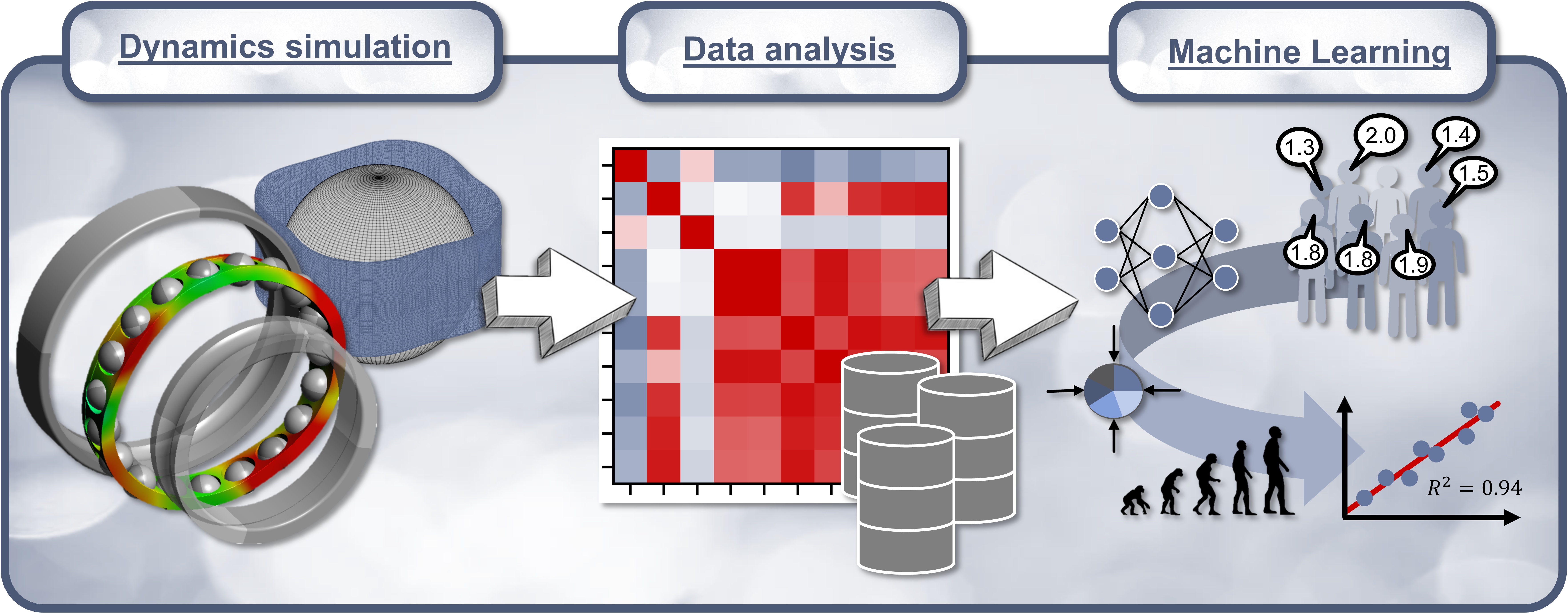
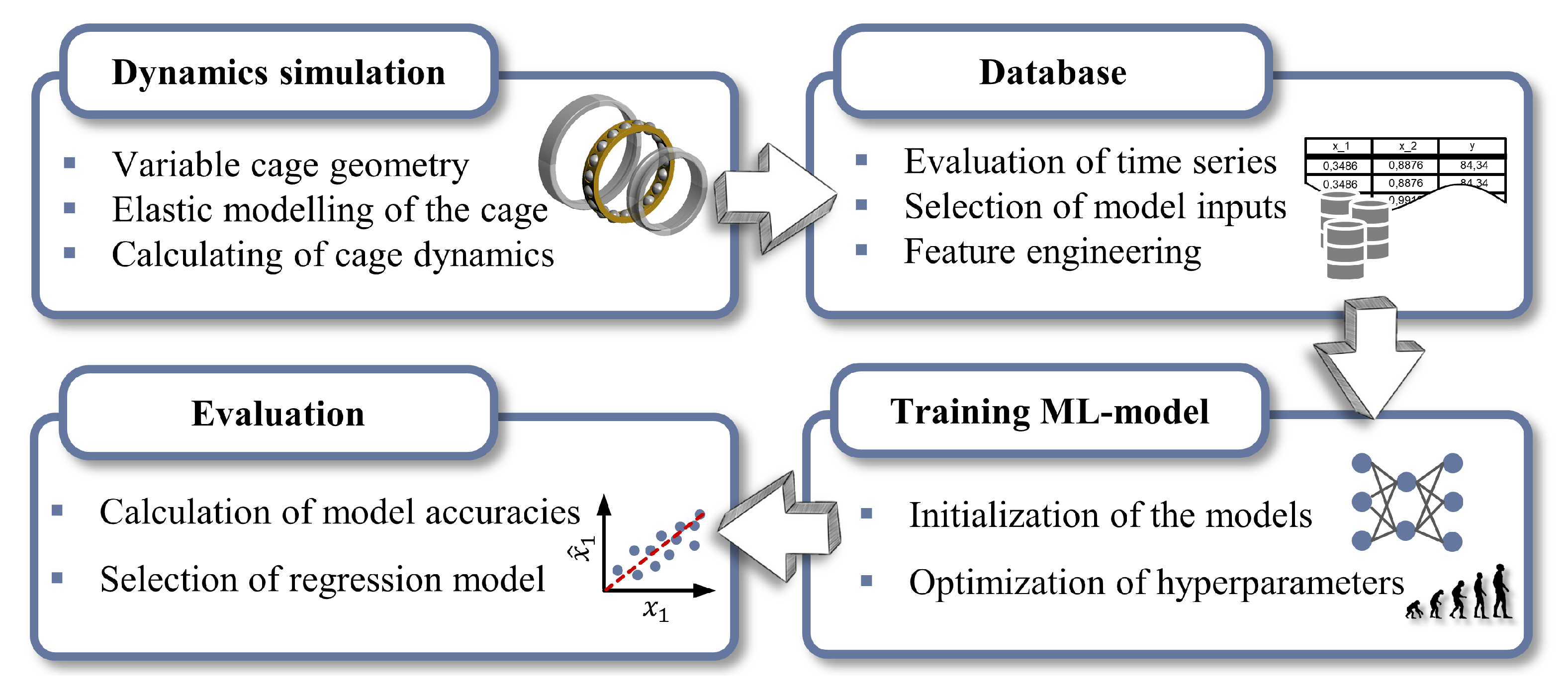
In previous research investigations [21], it was possible to quantify the dynamics of the cage for different operating conditions, but this was usually completed in isolated cases within the framework of complex numerical calculations or tests. A method for the time-efficient estimation of the quantitative dynamic behavior of rolling bearing cages for certain cage properties and rolling bearing loads is not yet available. The aim of this paper is to present a procedure for predicting the dynamics of a rolling bearing cage in an angular contact ball bearing using dynamics simulations and regression machine learning algorithms. This enables time-efficient estimation of the dynamics for the intended application during the development and selection of rolling bearing cages and also for operating conditions that are not directly included in the training data.

2. Materials and Methods

2.1. Methodology

The application of machine learning regression methods to predict the dynamics of a rolling bearing cage requires data representing the correlation between the varied parameters and the calculated cage dynamics. The starting point was the multi-body simulation model defined in the software Caba3D [22,23]. The calculation parameters of the model such as initial and boundary conditions, friction models, and elastic modeling of the cage are described in Section 2.2. The geometry of the cage as well as the bearing load and rotational speed were modified with the help of a comprehensive simulation plan using the design of experiment, see Section 2.3. A Latin hypercube sampling was used to ensure that the varied parameters are distributed uniformly in the entire mathematical space defined by previously specified boundaries [24]. The limits of the simulation plan were chosen so that the operating conditions prevailing in reality are mainly covered. On the basis of the uniformly distributed parameter values in the simulation plan, the correlations between the parameters can be efficiently learned by the algorithm. After performing the calculations, the simulation results were used to determine the input and output parameters and thus the data sets for machine learning, see Section 2.4. Characteristic values such as the Cage Dynamics Indicator (CDI) defined by Schwarz et al. [21] were derived from the calculated time series, which can be used for the assessment of the cage dynamics and as target values for machine learning. Artificial neural networks (ANN) [25], random forest (RF) [26], and XGBoost [27] were applied to predict the target variables based on the varied calculation parameters, see Section 2.5. The optimization of the hyperparameters of the used algorithms was performed as part of the training process using an evolutionary algorithm (EA) [28]. Finally, the predictions of the optimized models for test data sets were compared so that the most suitable algorithm could be selected. Figure 1 illustrates the procedure for generating a regression model for the prediction of characteristic values representing cage dynamics.

2.2. Calculation of Bearing Cage Dynamics

The multi-body simulation software Caba3D [29] developed by Schaeffler Technologies AG & Co. KG was used to determine the rolling bearing dynamics. This tool allows the calculation of the dynamics of all rolling bearing components for a previously defined time step and simulation time using a Runge–Kutta-method for performing the numerical time step integration. The results of the multi-body simulation include the kinematics (position, velocity, and acceleration in all degrees of freedom) of the rolling bearing components as well as contact results (pressures, relative velocities, etc.) and node displacements of the elastically modeled cage [23].

The discretization of the contacts rolling element/raceway as well as cage/ring was achieved by means of slices. Contact results such as pressure or forces were calculated for each of the slices and thus resolved locally [22]. For the contact calculation between rolling element and cage pocket, the ’node-to-surface model’ was used. This approach determines the contact results using the surface nodes of the finite element (FE) model of the cage and the slices of the rolling element. This allowed the elastic deformations of the cage and their effects on the contact conditions to be determined during the calculation [22]. An elastohydrodynamic model with consideration of mixed friction and the surface roughness was used for the calculation of the friction between rolling elements and raceways. The lubricant film thickness was calculated according to Dowson-Higginson [30]. Coulomb’s friction law was used to calculate the frictional force in the contact between the cage and the other bearing elements.

The calculation of the node displacements of a FE model of the rolling bearing cage with several thousand degrees of freedom would be too computationally intensive in the context of a multi-body simulation. Therefore, a model order reduction according to Craig and Bampton [31] was performed to consider the node displacements of the FE model during the dynamics simulation. This allows the number of degrees of freedom to be significantly reduced without a meaningful degradation in accuracy [29]. For the reduction in the FE model, eigenfrequencies up to 20 kHz and a maximum of 100 eigenmodes were considered. The deviation of the eigenfrequencies from the original model and thus the quality of the reduced FE model was verified using various quality criteria (e.g., modal assurance criteria and normalized relative eigenfrequency difference [29,32]).

The modeling considered the angular contact ball bearing without adjacent machine elements consisting of two bearing raceways, the rolling elements, and the outer ring guided cage, see Figure 2.

The degrees of freedom of the outer ring were disabled, while the other rolling bearing components could move along all six degrees of freedom. The angular contact ball bearing was loaded axially ($F_{\mathrm{x}}$) and radially ($F_{\mathrm{y}}$) by a force on the inner ring. Further parameters important for the calculation can be found in

Table 2. Calculation information of the simulation model.

Group	Property	Value
Integration	Integration method	Runge–Kutta
	Output time step	0.0001 s
	Calculation time	1.0 s
Cage properties	Cage guidance type	rib
	Cage material	fibre reinforced phenolic resin
Bearing properties	Inner diameter	90 mm
	Outer diameter	140 mm
	Pitch diameter $d_{\mathrm{p}}$	115 mm
	Rolling elements	19 balls
	Rolling element diameter	15.875 mm
	Ring and ball material	100 Cr6
	Contact angle $\alpha$	15°
	Static load capacity $C_{0,\mathrm{r}}$	51 kN

.

The data-driven approach to employ machine learning methods for cage dynamics prediction requires a high-quality set of data. The source of the data is the multi-body simulation software Caba3D, for which a high correlation with the real cage motion has already been found several times [10,14,21] and is therefore considered as a reliable source for the generation of datasets. Schwarz et al. used a test rig specially developed for testing cages of rolling bearings and high-speed cameras for optical measurement of cage dynamics. As in the calculations, cage instability could be observed in the experiment. For the shape, amplitude, and frequency of the cage deformation, high agreement was found with the measurement results [21].

2.3. Simulation Plan for the Cage Geometry and Bearing Load

Twenty cage variants were generated for the angular contact ball bearing, and their dynamic behavior was calculated for 100 different operating conditions using multi-body simulations as described in Section 2.2. In total, 2000 dynamics simulations were performed. Figure 3 illustrates the geometry parameters used to generate different cage designs. The chosen parametrization of the cage geometry enables the shape to be represented as generically as possible by 7 parameters. This allows cages with different properties to be created in the given design space and their dynamic behavior to be investigated. Using the parameter $d_{\mathrm{g}}$, the clearance between the cage and the outer ring and thus the guidance clearance can be influenced, see Figure 3a. The cross-section of the cage is defined by the height $h_{\mathrm{c}}$ and width of the cage $b_{\mathrm{c}}$, see Figure 3a. Both parameters affect important properties such as mass, moment of inertia, and stiffness of the cage. The shape of the cage pocket was varied using the parameters $c_0$, $c_1$, $c_2$, and $c_3$, which represent the pocket clearance along the circumference, see Figure 3b.

By choosing the pocket shape parameters, the pocket clearance of the cage on the one hand and the contact point between cage and the rolling element on the other hand can be influenced. The pocket clearance has a significant effect on the cage dynamics, as the number of contacts to the rolling elements increases with decreasing pocket clearance and can cause highly dynamic cage movements [21]. The contact point between the rolling element and the cage defines the direction of the normal and frictional force vector in the contact and finally the direction of the cage acceleration.

Using the geometry parameters, a total of 20 different cage variations were created using Latin hypercube sampling. The boundaries for the sampling shown in

Table 3. Minimum and maximum values of the parameters for the Latin hypercube sampling.

Parameter	Minimum	Maximum
Load ratio R	0.25	10
Equivalent dynamic bearing load P in N	1000	10,000
Torque on inner ring $T_{\mathrm{z}}$ in Nm	10	50
Rotational speed inner ring $n_{\mathrm{i}}$ in rpm	1000	9000
Friction coefficient rolling element/cage ${\mu }_{\mathrm{c}}$	0.05	0.35
Pocket shape parameters $c_0,c_1,c_2,c_3$ in mm	0.1	0.35
Cage width $b_{\mathrm{c}}$ in mm	19	23
Cage height $h_{\mathrm{c}}$ in mm	4	8
Guidance diameter $d_{\mathrm{g}}$	122	124.2

were chosen in such a way that there are no dependencies between the cage design parameters. For the smallest guidance diameter $d_{\mathrm{g}}$ and largest cage height $h_{\mathrm{c}}$, the clearance cage/inner ring is greater than the clearance cage/outer ring, and the same guidance type is provided.

Besides the modifications of the cage geometry, the load on the rolling bearing was also modified using an additional Latin hypercube sampling. The forces acting on the inner ring were varied using the load ratio R and the equivalent dynamic bearing load P. Based on the two parameters in Equations (1) and (2), the forces $F_{\mathrm{x}}$ and $F_{\mathrm{y}}$ to be defined in the simulation can be calculated. In addition to the forces, the inner ring was also loaded by the torque $T_{\mathrm{z}}$ acting around the z-axis, see Figure 2. The frictional force in the rolling element/cage contact was varied via the coefficient of friction ${\mu }_{\mathrm{c}}$.

$$P=X·F_{\mathrm{x}}+Y·F_{\mathrm{y}}$$

(1)

$$R=\frac{F_{\mathrm{x}}}{F_{\mathrm{y}}}$$

(2)

The speed of the inner ring $n_{\mathrm{i}}$ was also taken into account in the sampling. The kinematic speed of the rolling elements $n_{\mathrm{r}}$ and the cage $n_{\mathrm{c}}$ at the beginning of the simulation were determined for the initial time step by the Equations (3) and (4) depending on the defined inner ring rotational speed [33].

$$n_{\mathrm{r}}=-\frac{n_{\mathrm{i}}}{2}·\left(\frac{d_{\mathrm{p}}}{d_{\mathrm{re}}}-\frac{d_{\mathrm{re}}·{\cos }^2\left(\alpha \right)}{d_{\mathrm{p}}}\right)$$

(3)

$$n_{\mathrm{c}}=\frac{n_{\mathrm{i}}}{2}·\left(1+\frac{d_{\mathrm{re}}·\cos \left(\alpha \right)}{d_{\mathrm{p}}}\right)$$

(4)

A simulation plan consisting of a total of 100 operating conditions (inner ring rotational speed, force and torque on the inner ring, and friction coefficient in the rolling element/cage contact) was created using the boundary values in Table 3 and Latin hypercube sampling. Simulation models were generated for each of the 20 cage variants according to the same operating conditions defined by the created simulation plan, so that a total of 2000 dynamics simulations were performed.

2.4. Features and Targets for Machine Learning

The input and output parameters for machine learning were derived from the calculation models and results and formed the database. The input parameters were structured by mechanical and geometrical properties of the cage as well as the loading parameters and the resulting class of the cage motion (according to Schwarz et al. [21]), see

Table 4. Features for the machine learning model.

Group	Property	Symbol
Mechanical and material properties	Weighted area moment of inertia	$\tilde{I}$
	Weighted cross-sectional area	$\tilde{A}$
	Cage mass	m
	Cage moment of inertia	$J_{\mathrm{x}}$, $J_{\mathrm{y}}$
Geometric properties	Pocket shape parameters	$c_0,c_1,c_2,c_3$
	Pocket clearance circumferential	$c_{\mathrm{c}}$
	Pocket clearance axial	$c_{\mathrm{a}}$
	Guidance clearance	$c_{\mathrm{g}}$
Load parameter	Axial Force	$F_{\mathrm{x}}/C_{0,\mathrm{r}}$
	Radial Force	$F_{\mathrm{y}}/C_{0,\mathrm{r}}$
	Torque	$T_{\mathrm{z}}/(C_{0,\mathrm{r}}·d_{\mathrm{p}})$
	Rotational speed inner ring	$n_{\mathrm{i}}$
	Coefficient of friction	${\mu }_{\mathrm{c}}$
Predicted cage motion	Cage motion class	C

. Stiffness as a mechanical property is defined using a weighted area moment of inertia and cross-sectional area of the cage as input parameters. The weighting of the cross-section properties in the pocket and in the bar is based on a nonlinear function that provides a disproportionate amount of the area moment of inertia and the cross-sectional area in the cage pocket according to Schwarz et al. [21]. The cage mass and the mass moments of inertia complement the mechanical properties. The geometrical properties consist of the pocket shape parameters and the pocket and guidance clearance of the cage. The mechanical and geometrical parameters represent the essential properties that can be derived from a given cage geometry. The axial and radial loads, as well as the torque acting on the inner ring, were defined as relative quantities in relation to the basic static load rating $C_{0,\mathrm{r}}$ and the pitch diameter $d_{\mathrm{p}}$ as input parameters. Thus, the database can be supplemented by calculation results of other bearing sizes in the future. The cage motion class is represented by one of the basic observable cage motion types, “unstable”, “stable”, or “circling”, and was determined using Quadratic Discriminant Analysis based on the simulation results. The movement types differ in their dynamic behavior and can be classified based on their kinematics [34]. The cage motion type can also be predicted with high reliability by the classification algorithm AdaBoostM1 using the input parameters of the simulation [21]. However, the cage motion class provides information about the dynamics of the cage in a qualitative level. By extending the prediction using a regression algorithm, the relevant kinematic results can be specified more precisely.

The Cage Dynamics Indicator (CDI) defined by Schwarz et al. [21] contains all necessary parameters for the assessment of the cage dynamics and was used as the target of the regression task. The median (med) and the quantile distance (qd) indicate the distribution of the motion quantities contained in the CDI and were determined from the calculated time series. For the evaluation of the cage motion, the $\Omega$-ratio, the cage coordinates normalized to the guidance or pocket clearance ${\tilde{x}}_{\mathrm{c}}$, ${\tilde{y}}_{\mathrm{c}}$, and ${\tilde{z}}_{\mathrm{c}}$, the rotational ratio ${\tilde{n}}_{\mathrm{c}}$, and the equivalent deformation force $F_{\mathrm{e}}$ were used.

In addition to the CDI, the output parameters include the median of the frictional torque $T_{\mathrm{f}}$, the median of the contact forces on the cage $|F_{\mathrm{c}}|$ and the median of the translational acceleration $|a_{\mathrm{c}}|$ of the cage. In total, the output parameters for the regression algorithm consist of 10 parameters, which can be used to assess the cage dynamics as well as the energy efficiency of the bearing. In previous research papers, the CDI has been used as a key figure to assess the cage motion calculated by the dynamics simulation [14,21,34]. In this contribution, machine learning methods will be used to predict the CDI in order to accurately assess cage dynamics.

A strong scatter of the target variables reduces the prediction accuracy of the algorithms. Therefore, an anomaly detection for each motion class identified outliers of the target variables and removed them from the database. A density-based approach developed by Breunig et al. was used for anomaly detection. The local outlier factor (LOF) determines the degree of isolation of a data set compared to the immediately neighboring data sets [35].

2.5. Regression Algorithms and Hyperparameter Optimization

In this paper, the prediction accuracy of three different regression algorithms (Random Forest, XGBoost, and Artificial Neural Networks) used to estimate rolling bearing cage dynamics are compared. The hyperparameters of the models were determined by an EA as part of an optimization of the prediction accuracy [28].

RF is an ensemble method based on the ‘wisdom of the crowd’ paradigm. According to this, a prediction made by a large number of different persons/models achieves better results than the prediction of a single person/model. Accordingly, an RF regressor contains multiple regression trees that learn the regression problem using different sub-sets of the original training data. These sub-sets are regenerated by bagging for each regression tree. The degree of randomness is further increased by using only a random selection of features for training the decision trees. Random components (bagging or feature selection) reduce the model’s tendency to overfit the training data [36].

Gradient boosting is another ensemble method developed by Friedman [37]. In an iterative process, multiple regression trees are trained. The training process of a decision tree depends on predictions and loss of the already trained decision trees in the ensemble. One implementation of gradient boosting is XGBoost (extreme gradient boosting) [27], which was used for predicting cage dynamics in the present case. As the regression algorithm in XGBoost is designed to predict only a single value, one model was trained for each output parameter. However, this allows interactions of the targets to be represented less effectively than with the random forest regressor.

ANNs are widely used algorithms for classification and regression in the field of machine learning. The input value of a neuron results from the weighted sum of the output values of the neurons of the previous layer and a so-called constant bias value. The neuron’s input value is converted into the output by a nonlinear activation function. During the training of the ANN, the weights as well as the bias values are optimized so that the relationship in the training data between the input values and the output values can be predicted as accurately as possible [38]. For the prediction of the cage dynamics in this paper, an ANN consisting of a total of five layers was trained using the training algorithm Adam [39]. The target variable of the optimization procedure is the mean square error (MSE) between the ANN’s predictions and the target values contained in the training data.

For the ML algorithms, hyperparameters such as the ANN’s number of neurons per layer need to be specified. With the help of an EA, the hyperparameters were determined so that the prediction accuracy of the models were optimized. The remaining parameters of the models are listed in Appendix A. The EA uses mechanisms of biological evolution such as selection, recombination and mutation to improve the fitness (metric for assessing regression results, e.g., coefficient of determination $R^2$) of the individuals (set of hyperparameters) contained in a population (amount of individuals) for a predefined number of generations, see Figure 4. Starting from an initial population generated by Latin hypercube sampling, the fitness of each individual is determined. The fitness of the individuals and target value of the EA was represented by the mean $\overline{R^2}$ according to Equation (5). Using a K-fold ($K=5$) cross-validation, a total of K validation data sets were generated from the training data for fitness evaluation. The data set was randomly split so that 85% is used for hyperparameter optimization as well as the cross-validation contained within the loop and 15% for subsequent testing of model predictions. $\overline{R^2}$ was calculated by evaluating the arithmetic mean of the $R^2$ for each validation data set and target variable. The prediction accuracy for the validation data is an indicator of the generalization capability of the model, which can be finally evaluated after training by the test data sets.

$$\overline{R^2}=\frac{1}{K}·\frac{1}{N}·\sum _i^K\sum _j^N{R}_{ij}^2$$

(5)

The $R^2$ of each output parameter was calculated by Equation (6) using the predictions of the algorithm ${\widehat{y}}_{\mathrm{i}}$, the target parameter according to the test data $y_{\mathrm{i}}$, and its arithmetic mean $\overline{y}$. Thus, $R^2$ can reach a maximum value of 1 in case of an error-free prediction of the algorithm.

$$R^2=1-\frac{{\sum }_i{(y_i-{\widehat{y}}_i)}^2}{{\sum }_i^{}{(y_i-\overline{y})}^2}$$

(6)

After calculating the fitness of the initial population, the evolutionary process consisting of selection, recombination, mutation, and evaluation of fitness was repeated in a given number of generations. Individuals for recombination were selected by the fitness proportional method stochastic universal sampling. Each individual received an area proportionate to its fitness value on a wheel. By spinning the wheel once and with n arrows equally distributed around the circumference, n individuals were selected by the pointers. Recombination was performed in pairs for the selected individuals. The list of hyperparameters of two individuals for mating were separated at two points and the new resulting individuals were defined by alternating the combination of the sections, see Figure 4. After recombination, mutation was performed for each parameter contained in the individual by a uniformly distributed random variable. Mutation served to generate new parameter specifications in the population and was performed with a previously defined probability. The individuals produced by recombination and mutation, as well as the best individual from the previous population (elite), formed the new population for the following generation.

After a predetermined number of generations, the model with the highest fitness and best prediction accuracy for the test data was returned by the EA. The parameters controlling the behavior of the EA can be taken from

Table 5. Parameters of the EA for the optimization of the hyperparameters of the regression algorithms.

Parameter	Value	Parameter	Value
Number of generations	30	Population size	50
Elite individuals	1	Crossover probability	0.8
Mutation probability	0.15

.

Table 6. Hyperparameters of the regression models optimized using the EA.

Model	Parameter	Minimum	Maximum
XGBoost	Max depth	20	200
	Number of estimators	100	1500
	Learning rate	0.0001	0.01
	L1 regularization	0.0001	0.9
	L2 regularization	0.0001	0.9
	Minimum loss reduction for tree split	0.00001	0.2
Random Forest	Max depth	20	200
	Number of estimators	100	1500
	Minimum samples required for a leaf	2	10
	Maximum number of features for a split	10	17
	Maximum number of leaf nodes	10	500
	Minimal cost-complexity pruning	0	0.5
ANN	Number of neurons in layer 1	100	600
	Number of neurons in layer 2	100	600
	Number of neurons in layer 3	100	600
	Number of neurons in layer 4	100	600
	Learning rate	0.0001	0.9
	Activation function	ELU, RELU, Leaky_RELU

shows the hyperparameters of the algorithms and components of the individuals as well as the range of the parameters considered during optimization. The ranges of the hyperparameters were chosen to be comparatively large in order to provide as many parameter combinations as possible. Large ranges of the hyperparameters increase the risk of overfitting (e.g., large number of neurons contained in the ANN). However, overfitting was avoided, including in the training methods of XGBoost and ANN, by using evaluation datasets. Based on the predictions for the evaluation datasets that were not used directly for training, it is determined whether overfitting is present in the current state of the training process. No evaluation dataset was used for Random Forest, because the algorithm generally has a low tendency to overfit the training data [36].

3. Results

3.1. Dynamics Simulation Results

The results of the dynamics simulations contain time series that include dynamics of the cage as well as the rolling elements. Figure 5 shows an example of the dynamic behavior of a cage for different operating conditions of the bearing. In the qualitative assessment of cage dynamics, a fundamental differentiation is made between “unstable”, “stable”, and “circling” cage motions [21,34]. These types of movements could also be observed for the cages investigated. 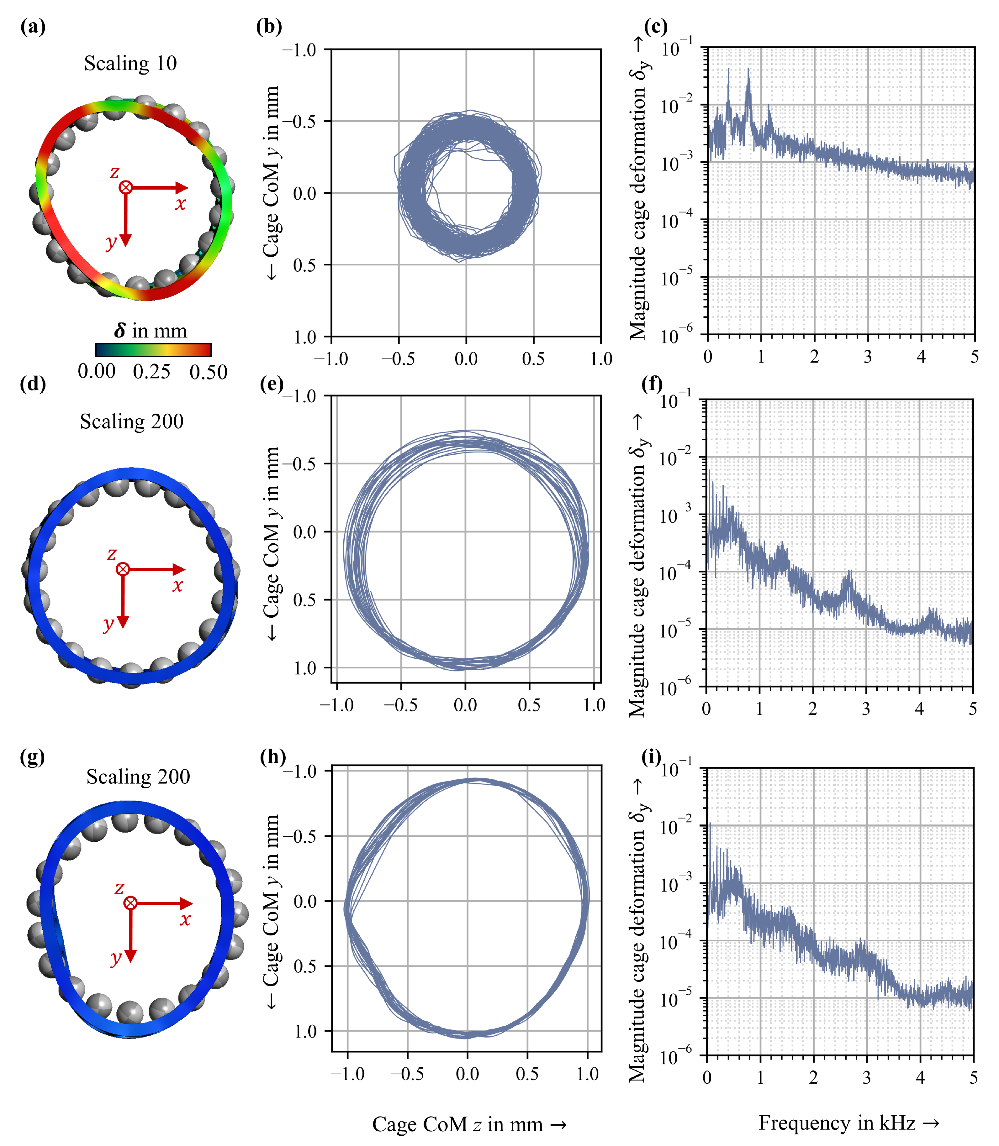Figure 5a–c illustrates an example of an unstable cage motion (loading conditions ${\mu }_{\mathrm{c}}=0.21$, $F_{\mathrm{x}}=-8058$ N, $F_{\mathrm{y}}=1077$ N, $n_{\mathrm{i}}=8263$ rpm $T_{\mathrm{z}}=48$ Nm), that is characterized by high dynamics as well as severe and high-frequency cage deformations. The cage was pressed against the outer ring and strongly deformed. This led to the diameter of the circular center of gravity trajectory being significantly larger than in the other two calculations. In addition, high contact forces caused frictional losses, which significantly impair the energy efficiency of the rolling bearing. In the case of stable cage motion (loading conditions ${\mu }_{\mathrm{c}}=0.26$, $F_{\mathrm{x}}=-\mathrm{15,126}$ N, $F_{\mathrm{y}}=1636$ N, $n_{\mathrm{i}}=4407$ rpm $T_{\mathrm{z}}=14$ Nm), no significant deformations occurred and the dynamics of the cage were generally low, see Figure 5d–f. The contact forces between the cage and the rolling element and outer ring were also significantly reduced compared to an unstable motion, and therefore the frictional losses were also lower. The circling cage motion (loading conditions ${\mu }_{\mathrm{c}}=0.12$, $F_{\mathrm{x}}=-3030$ N, $F_{\mathrm{y}}=377$ N, $n_{\mathrm{i}}=6844$ rpm $T_{\mathrm{z}}=12$ Nm) is characterized by a circular motion of the cage center of mass that exhibits small variations in the rotational speed. The rotational speed of the cage center of mass corresponds to the speed of the rolling element set. The cage is pressed in a radial direction due to the centrifugal force acting, so that the number of contacts to the guidance rib and the contact force acting in the contact increase.

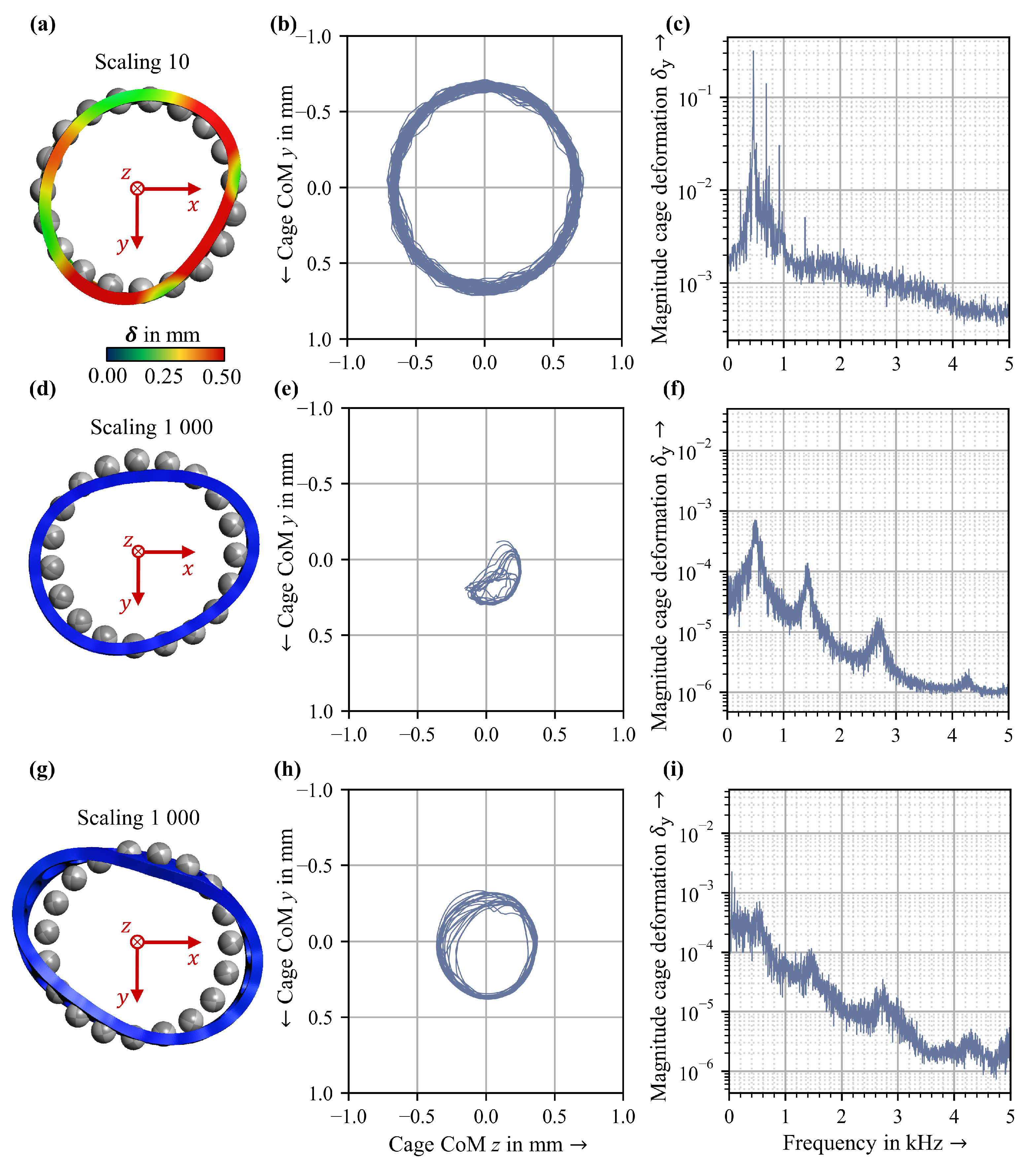
In addition to the load on the bearing, the geometry of the cage can also influence the dynamic response of the bearing. Figure 6 shows the cage dynamics for a load situation (${\mu }_{\mathrm{c}}=0.16$, $F_{\mathrm{x}}=-9655$ N, $F_{\mathrm{y}}=3718$ N, $n_{\mathrm{i}}=6844$ rpm $T_{\mathrm{z}}=16$ Nm) and three different cage geometries. The first cage variant performed a highly dynamic cage motion with severe deformations and a high rotational speed of the cage center of mass, see Figure 6a–c. A modification of the cage geometry (cross-section and shape of the cage pocket) for the other two variants and the same operating conditions led to circling cage motions in both cases. The amplitudes of the deformations were significantly smaller compared to the first cage variant and the larger amplitudes were shifted to the low frequency range, see Figure 6d–i.

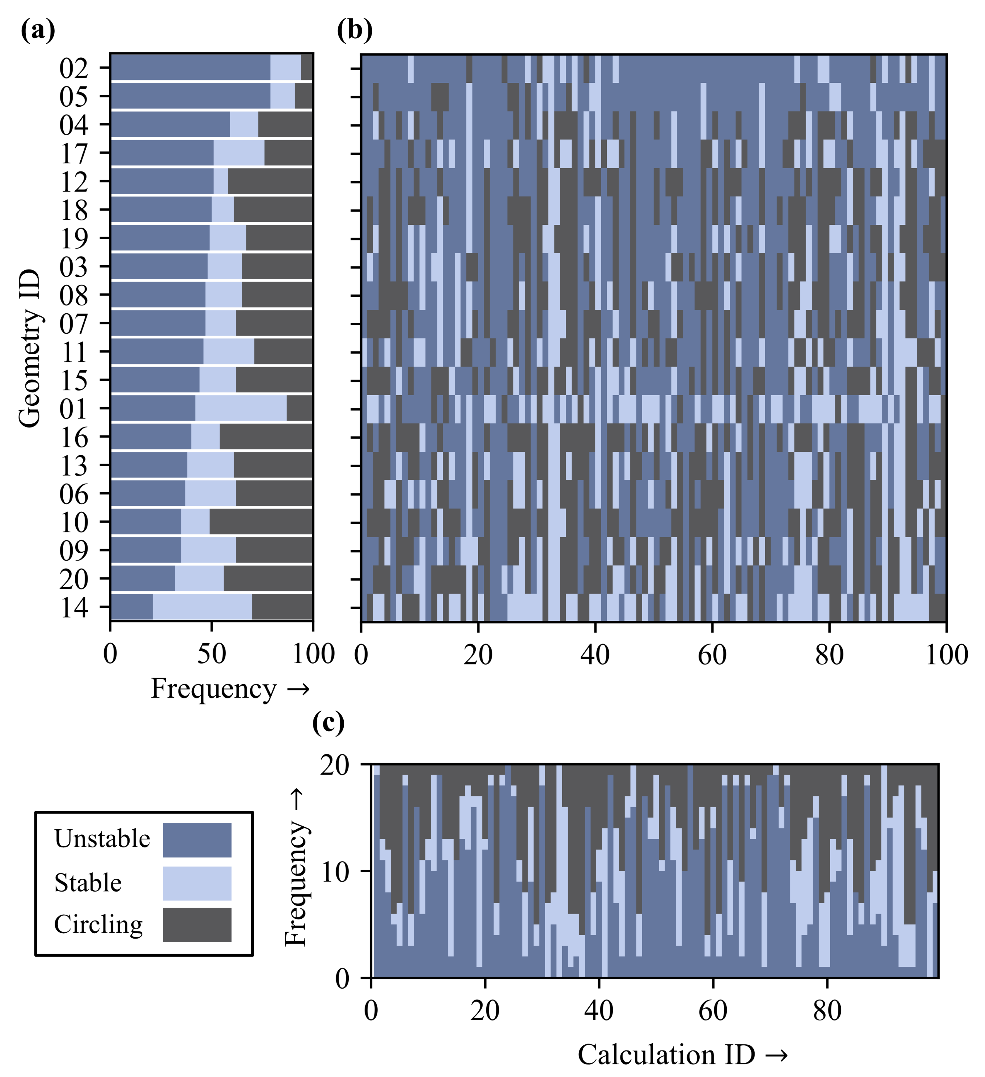
An overview of the simulations performed and the resulting cage motion types is shown in Figure 7. Certain cage geometries (ID 02 or 05) had a high proportion of unstable cage motions, while other cage variants exhibited a much lower tendency to unstable cage motions (ID 14 or 10). In addition, differences in the proportion of circumferential and stable cage movements were also evident for the different cage variants. The dynamic behavior of the cage variants illustrates the potential of the geometry parameters to positively influence the dynamics of the cage. A clear influence could also be identified in the loading conditions, as was found, for example, by Schwarz et al. [14]. However, as the operating conditions often cannot be influenced, these serve only as a reference for comparing the dynamic behavior of the cage geometries.

The simulation results were further processed so that the influence of cage geometry and bearing load was represented by a database consisting of input and target variables and could be used for machine learning.

3.2. Preprocessing of Calculation Results and Data Analysis

The calculated time series were the starting point for determining the targets for machine learning. For the evaluation of the cage dynamics, the time range $t=0.5...1$ s was analyzed to avoid unrepresentative cage motions due to the initial conditions at the beginning of the calculation.

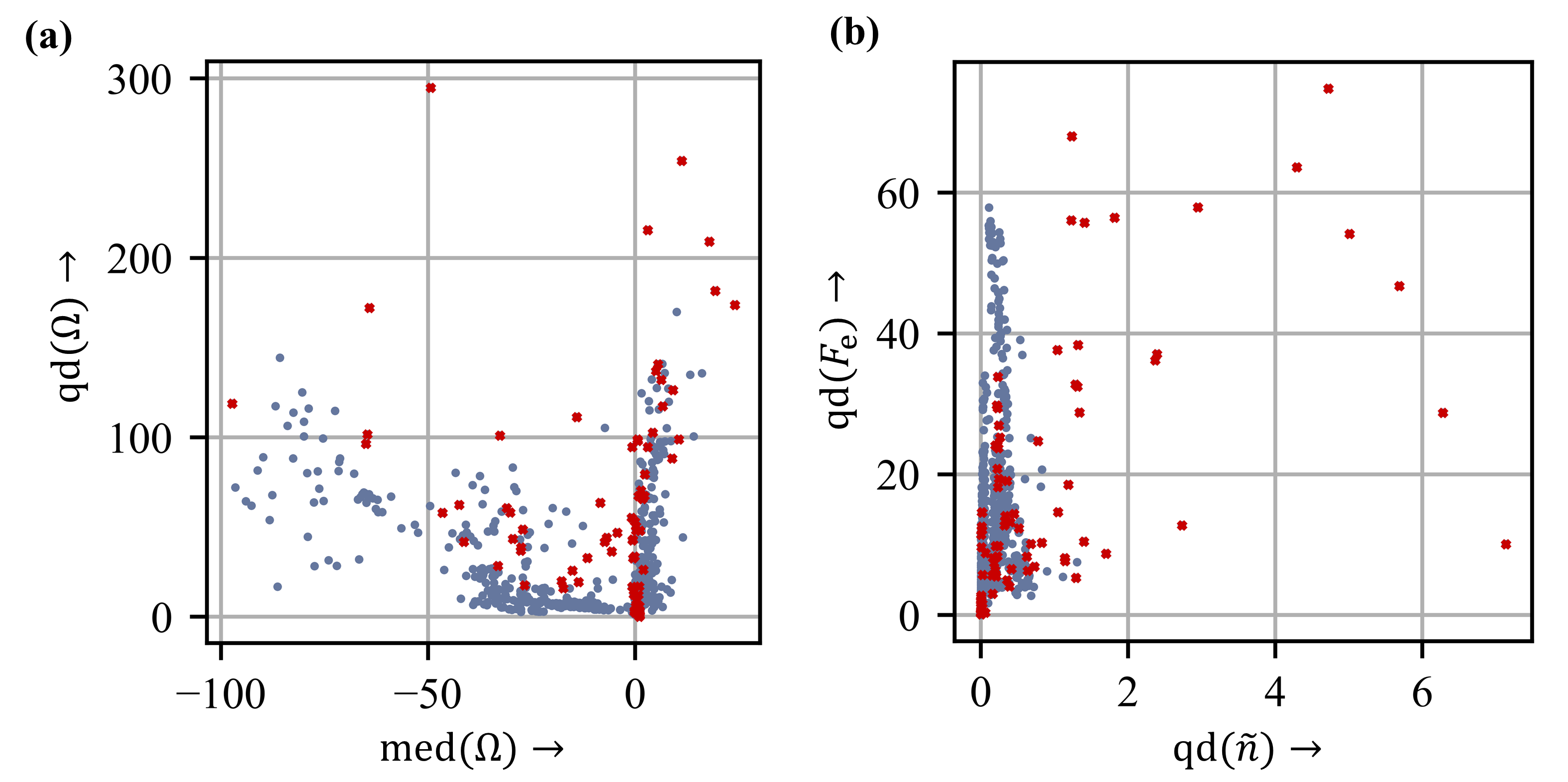
In addition it was checked whether the simulation results are suitable to be integrated into the database. Especially for simulations with high friction coefficients, a severe deformation of the cage occurred, which led to a termination of the simulation. Nonphysical results as the automatically generated inputs are out of a reasonable range for this application and were removed from the database. Using the density-based LOF approach, outliers in the database could be identified and removed. The LOF approach was applied to each of the classes “unstable”, “stable” and “circling”. Outliers with respect to the dynamic behavior typical for the respective classes were thereby identified. Figure 8 illustrates the outliers (red) and the remaining datasets (blue). Outlier detection reliably removed atypical cage movements, ensuring a high-quality database for machine learning. After preparing the simulation results, the database for machine learning contained a total of 1362 data sets.

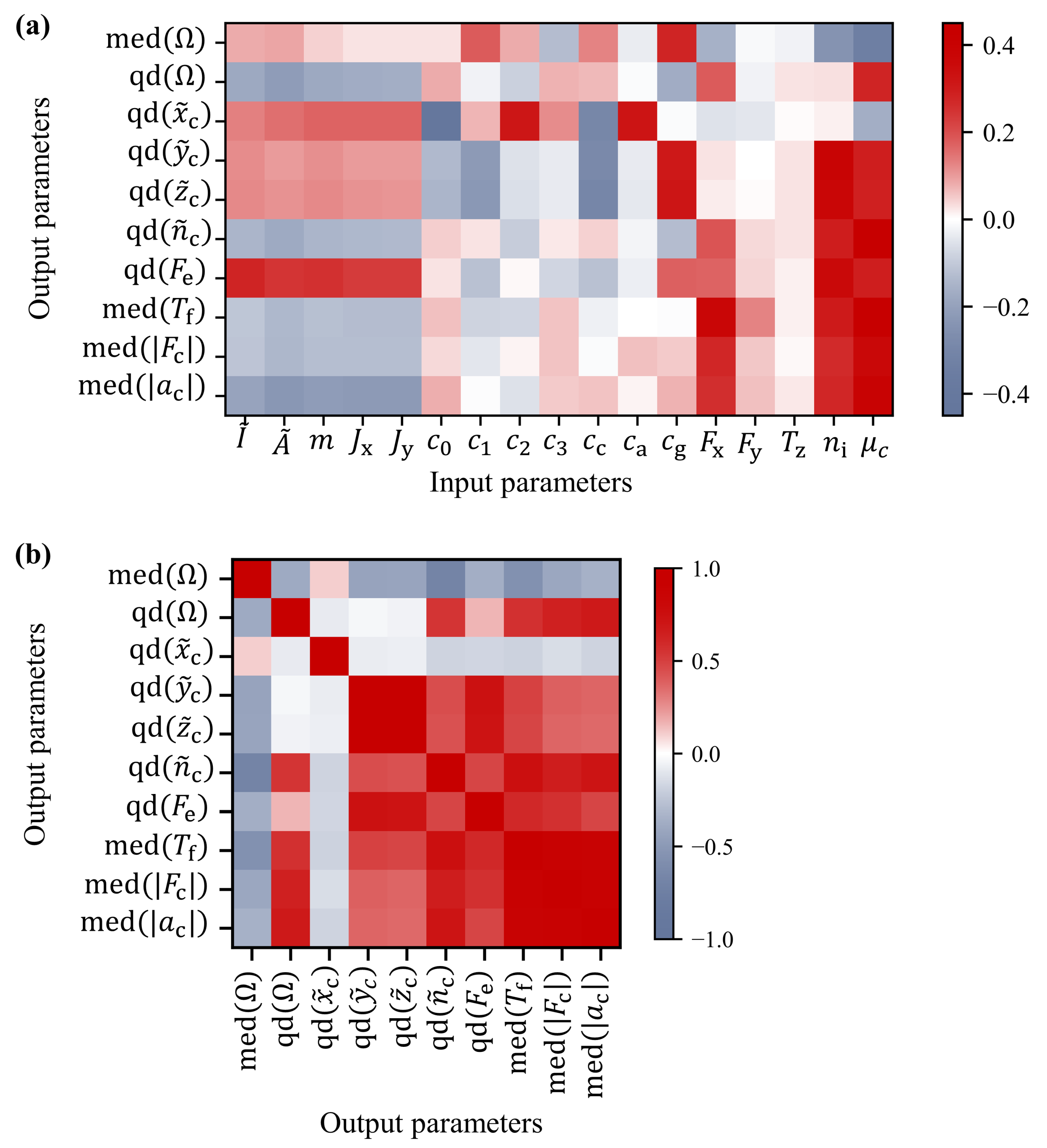
Figure 9 shows the correlation matrix for determining the qualitative relationship between input and output parameters. The mechanical properties of the cage (area moment of inertia $\tilde{I}$, mass m, area cross section $\tilde{A}$, and moment of inertia J) had similar values for the correlation coefficient and thus a related influence on the target parameters, see Figure 9a. A mathematical negative correlation existed between the mechanical properties and the center of mass acceleration of the cage $|a_{\mathrm{c}}|$. Accordingly, lower accelerations occur at higher masses of the cage, which can be justified by the inertia of the geometry. There is also a positive correlation between the cage mass and the equivalent force $F_{\mathrm{e}}$ representing the deformation of the cage. Thus, for the cages with larger masses, the equivalent deformation force tend to be larger. With respect to the bearing speed $n_i$ and friction coefficient ${\mu }_{\mathrm{c}}$, a mathematical positive correlation to cage acceleration, contact forces, and finally a highly-dynamic cage movement could be clearly determined. This is due to the increased relative velocity and frictional force in the contact between the cage and the other components, which leads to a stronger excitation of the cage and an increased tendency to highly dynamic movements.

Based on the matrix in Figure 9b, a mutual correlation of the output parameters was also evident. Highly dynamic cage movements are characterized by strong deformations of the cage, high accelerations, and a high frictional torque, for which reason these parameters exhibited a strong correlation. Due to the opposite movement of the center of mass in the case of unstable cage dynamics, there is a mathematical negative relationship between the median of the $\Omega$-ratio and the other parameters. The weak relationship of the normalized ${\tilde{x}}_{\mathrm{c}}$-coordinate of the cage to the other target quantities is also noticeable. The contact forces between the cage and the rolling element/rib point primarily in radial direction, which is the direction of the resulting acceleration. Therefore, the correlation between the quantile distance of the two non-axial coordinates is more significant, especially in the case of an unstable cage motion. The quantile distance of the $\Omega$-ratio also indicates a slightly lower correlation to the other parameters, but still stronger than the quantile distance of the ${\tilde{x}}_{\mathrm{c}}$-coordinate of the cage center of mass.

Although there were trends based on the correlation matrix that suggest the resulting dynamic behavior of the cage, the relationship is highly nonlinear due to interactions between the parameters. Therefore, the regression algorithms are trained in the following to learn the relationship between input and output parameters.

3.3. Evaluating Optimization and Regression Results

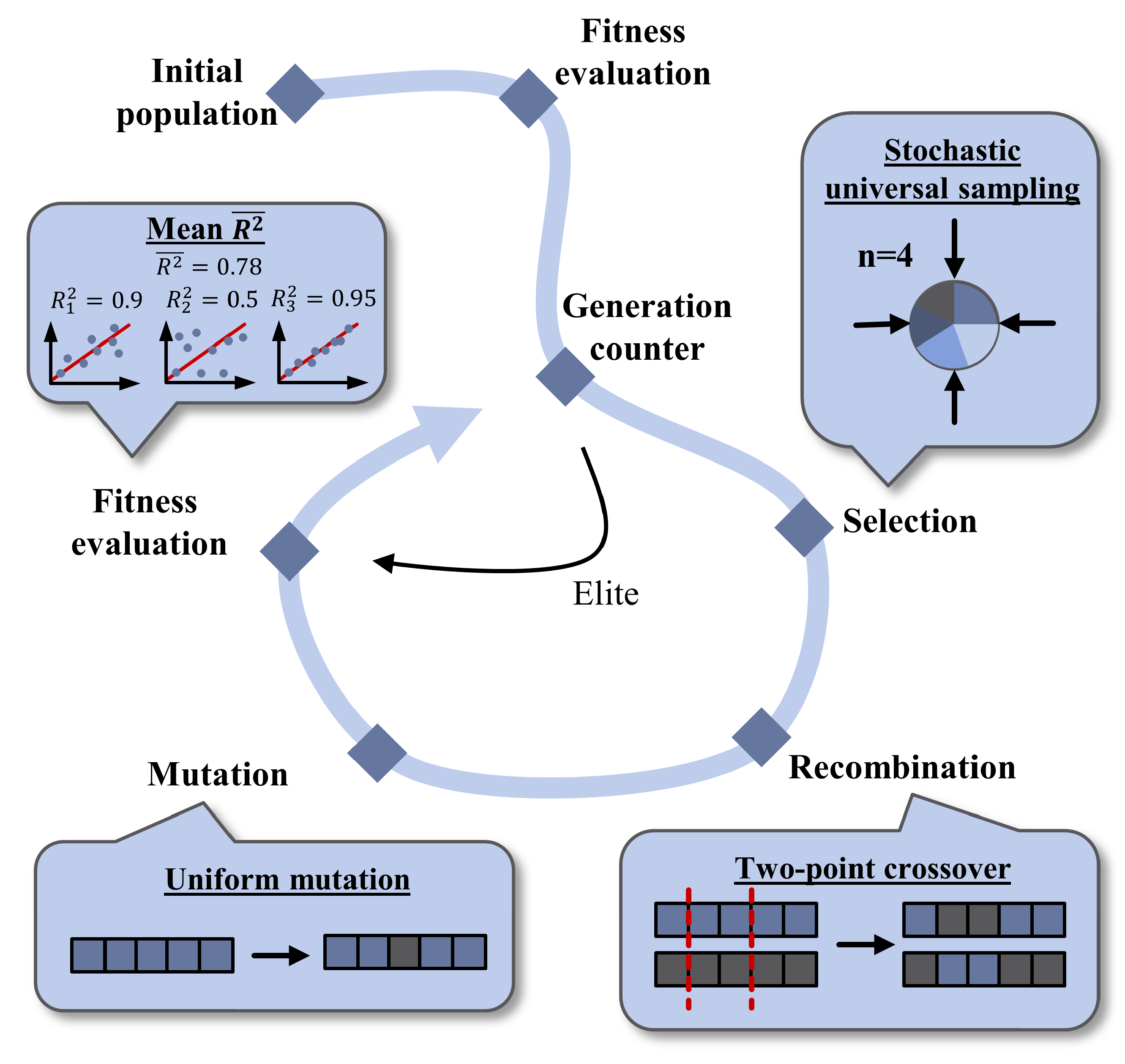
The EA determined the hyperparameters of the models to maximize the average coefficient of determination for the validation data sets. The best individuals or parameter combinations are shown in

Table 7. Optimized parameters of the regression models.

Model	Parameter	Minimum	Maximum	Value
XGBoost	Max depth	20	200	52
	Number of estimators	100	1500	832
	Learning rate	0.0001	0.01	0.045
	L1 regularization	0.0001	0.9	0.865
	L2 regularization	0.0001	0.9	0.791
	Minimum loss reduction for tree split	0.00001	0.2	0.021
Random Forest	Max depth	20	200	46
	Number of estimators	100	1500	812
	Minimum samples required for a leaf	2	10	2
	Maximum number of features for a split	10	17	17
	Maximum number of leaf nodes	10	500	441
	Minimal cost-complexity pruning	0	0.5	0.0009
ANN	Number of neurons in layer 1	100	600	447
	Number of neurons in layer 2	100	600	568
	Number of neurons in layer 3	100	600	577
	Number of neurons in layer 4	100	600	455
	Learning rate	0.0001	0.9	0.003
	Activation function	ELU, RELU, Leaky_RELU		Leaky_RELU

. A large number of neurons, or many estimators in the ensemble methods, increase the adjustable model parameters, the risk of overfitting to the training data, and poor prediction accuracy for test data. However, the hyperparameters causing overfitting were not chosen by the optimization to maximize the number of model parameters to reach high values for the prediction accuracy based on the training data. In general, this is a first indication that a generalization capable model was created by the training and optimization.

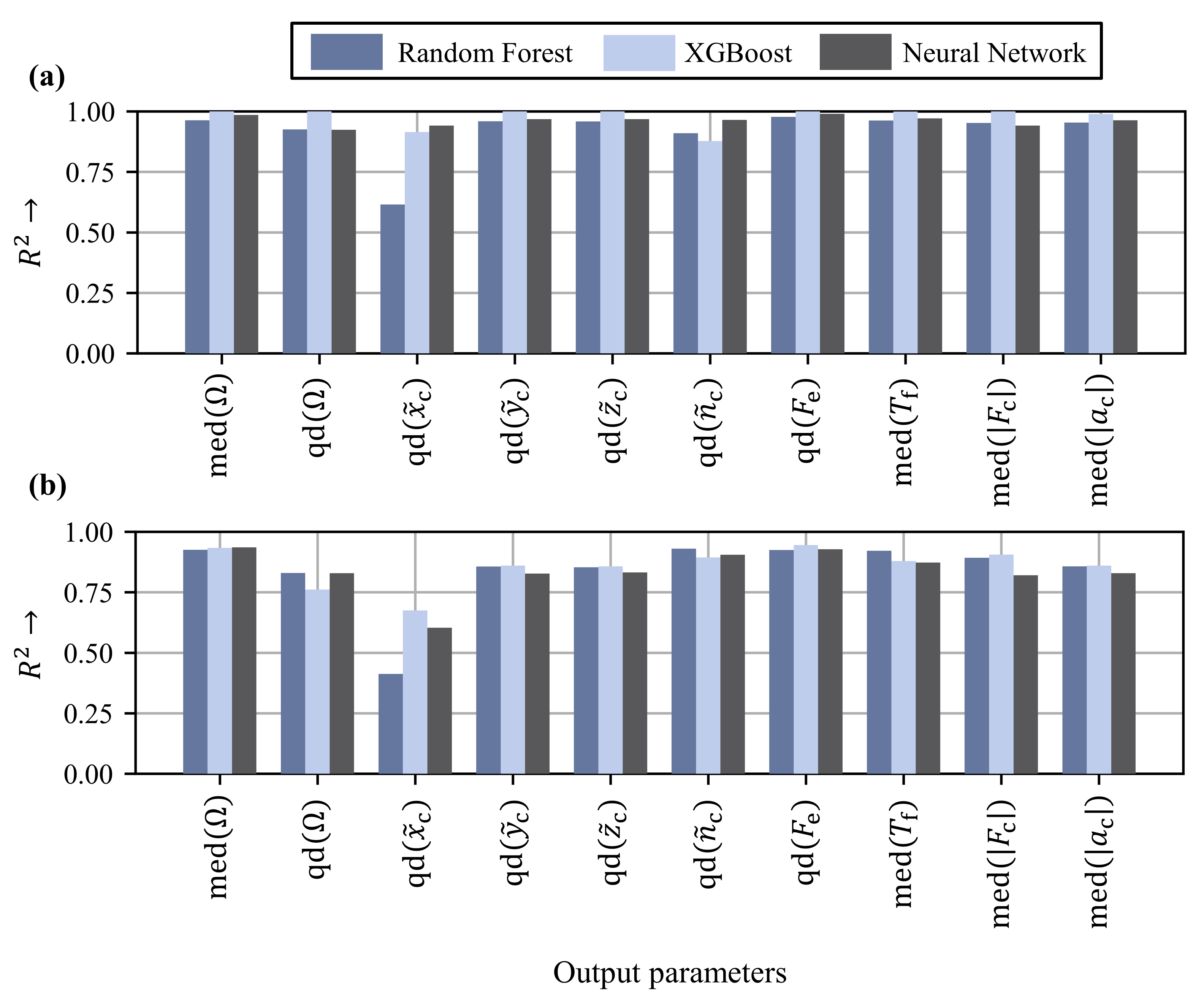
The hyperparameters optimized by the EA were used for training the algorithms. Afterwards, the models were evaluated using the coefficient of determination $R^2$ for test and training data, see Figure 10. For the training data, acceptable values for $R^2$ were obtained for all algorithms. The quantile distance for the normalized ${\tilde{x}}_{\mathrm{c}}$-coordinate of the cage reached $R^2\approx 0.41$ in the case of the random forest regressor, which is to be assessed as a medium correlation. The excitation of the cage, as well as the translational center of mass movement, occurs both for the contact of the cage to the rolling elements and to the rib in the radial direction. The relationship between the geometry and load parameters as well as the axial center of mass movement and finally the $R^2$ of the predictions were therefore lower compared to the other center of mass coordinates. Random forest regressor predicted very well for all target values, but reached a slightly lower $R^2$ compared to XGboost and the neural network for training data. The random components in the random forest algorithm (e.g., feature selection) prevent possible overfitting to the training data and led to slightly inferior prediction. The coefficients of determination $R^2\approx 1$ for XGBoost were very high and indicate a significant fit to the data sets.

The test datasets generally showed a lower coefficient of determination than the training datasets but were within an acceptable range apart from the quantile distance of the normalized ${\tilde{x}}_{\mathrm{c}}$ coordinate of the cage. qd(${\tilde{x}}_{\mathrm{c}}$) exhibited the worst values of $R^2\approx 0.41$ for the random forest and $R^2\approx 0.6$ the ANN. Thus, while qd(${\tilde{x}}_{\mathrm{c}}$) is suitable for assessing cage dynamics when derived from calculated time series, there is no strong correlation to bearing load or cage geometry. The difference in prediction accuracy for training and test data was lowest for random forest, which indicates a generalization of the model. However, the difference for XGBoost and the ANN was also in an acceptable range, which is also a sufficient generalization capability. All models reached comparable values for the coefficient of determination $R^2$ based on the test data sets and thus can be used equally for the prediction of cage dynamics. The best prediction values for $R^2$ based on the test data sets were obtained for the quantile distance of the equivalent deformation force $F_{\mathrm{e}}$, the median of the $\Omega$-ratio and the median of the friction torque $T_{\mathrm{f}}$ in the range of $R^2\in [0.90\dots 0.94]$. For the remaining target parameters, with the exception of qd(${\tilde{x}}_{\mathrm{c}}$), at least one of the models investigated achieved a coefficient of determination $R^2>0.8$ and sufficient prediction accuracy.

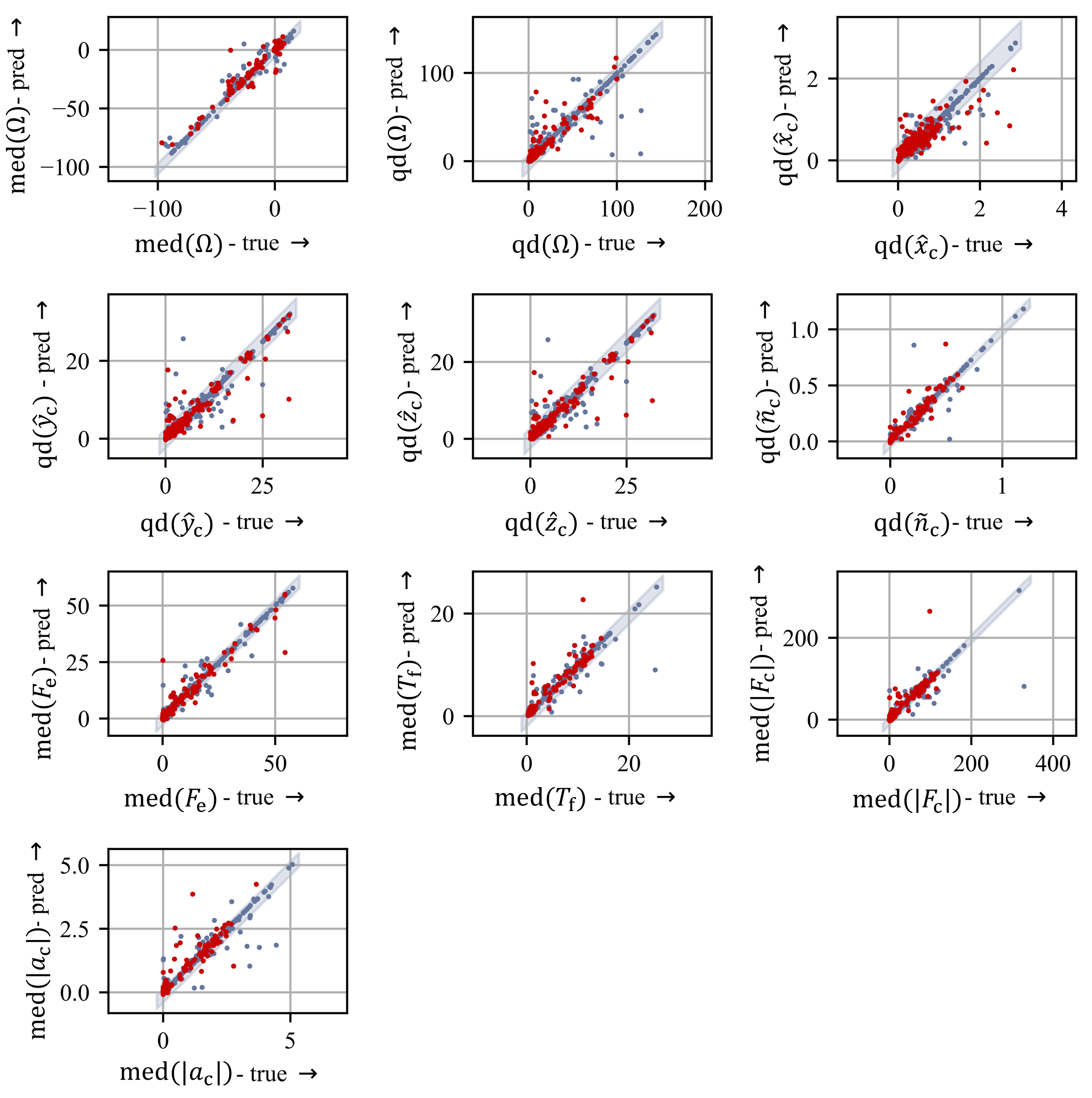
The scatter plot in Figure 11 shows, representative of the trained models, the predictions of the ANN compared to the true values in the training (blue) and test (red) data. As can be seen from the correlation matrix and the coefficient of determination, the predictions for the quantile distance of the axial coordinate of the cage qd(${\tilde{x}}_{\mathrm{c}}$) were considerably more scattered than the other target variables. For the quantile distance of the omega ratio, the deviation of the predictions from the test data sets was smaller, but a stronger, though still acceptable, scatter was also present here. For the remaining parameters, a good correlation was present, analogous to the $R^2$. The deviations are within a tolerable range, as can be seen by the intervals containing 90% of the errors determined for the test data (blue area).

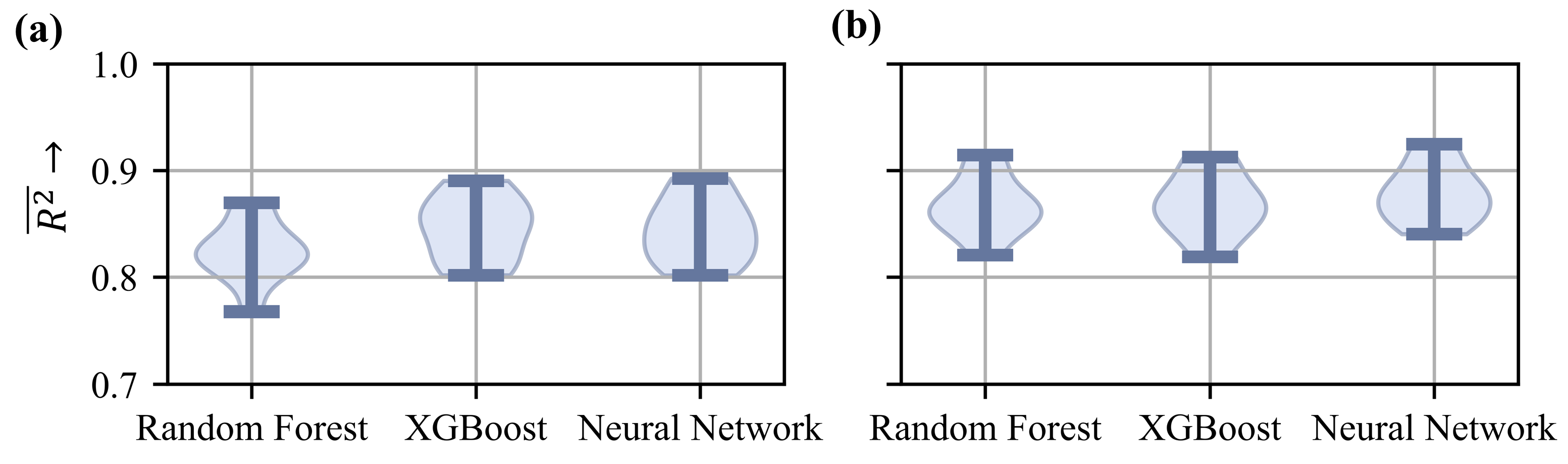
The hyperparameters obtained from the optimization by the EA were used to perform a 10-fold cross-validation. This allowed us to determine how strong the predictions of the algorithm differ depending on the used training and test data set, see Figure 12. Based on this, the sensitivity of the prediction results for different training and test data sets could be investigated. Figure 12 exhibits the distribution of the average prediction of the target values for the training data and a 10-fold cross-validation including (a) and excluding (b) the quantile distance of the cage coordinate ${\tilde{x}}_{\mathrm{c}}$ as regression target. For all three models, omitting the normalized coordinate improves the average prediction quality, as lower $R^2$ values are obtained for qd(${\tilde{x}}_{\mathrm{c}}$) than for the other values in all iterations of the cross-validation. The minima and maxima of $\overline{R^2}$ for the three models without considering ${\tilde{x}}_{\mathrm{c}}$ in the cross-validation were very similar and differ only slightly. As no obvious favorite could be identified based on the prediction accuracies, all three algorithms were suitable for predicting the cage dynamics with a comparable error tolerance.

4. Discussion

The results of the dynamics simulation illustrate the strong influence of the bearing load and cage geometry on the resulting cage dynamics, see Figure 7. Depending on the geometry, the tendency of a cage to highly dynamic and unstable cage movements varies significantly. However, the relationship between the geometry parameters and the resulting cage dynamics is very complex and difficult to determine using conventional methods of descriptive statistics, as can be seen from the covariance matrix in Figure 9. The complex relationship between the input and output parameters can basically be determined with the help of the investigated algorithms. Analyzing the prediction results for test data, it can be seen that for the quantile distance of the normalized center of mass coordinate ${\tilde{x}}_{\mathrm{c}}$ of the cage, mediocre prediction values could be obtained. As the frictional forces acting in contact between the cage and the other components accelerate the cage primarily in the bearing plane, the physical relationship between the input parameters of the model and the resulting axial cage motion is less than for the other parameters. The normalized ${\tilde{x}}_{\mathrm{c}}$ coordinate of the cage is thus less suitable for predicting the cage dynamics. Though, as a component of the multivariate metric CDI, which can be derived from calculated time series representing cage dynamics, ${\tilde{x}}_{\mathrm{c}}$ is a contribution to improve the classification performance.

The algorithms Random Forest, XGBoost, and ANN achieved similar values for the $R^2$ of the different target variables for the test data sets, see Figure 10. A 10-fold cross-validation exhibited that the differences between the models are small, and thus all algorithms are suitable for the prediction of the cage dynamics. The robustness of the predicted targets for a given cage geometry with respect to deviations from the true values can be improved by a large number of predictions by the regression algorithm with a subsequent statistical analysis. This reduces the influence of single incorrect predictions and improves the comparability of the dynamic behavior of different cage variants.

A transfer of the predictions to other rolling bearing sizes is possible in general. For this purpose, new training data must be generated and the existing database expanded. However, a similar effect on the cage dynamics can be expected, especially for the load conditions as shown, for example, by Schwarz et al. for various bearings [14,21]. Therefore, the amount of training data for the same bearing type and similar cage shapes can probably be lower than for the investigated angular contact ball bearing. In addition to the extension to other bearing types, other parameters can also be added as input variables, so that depending on the existing application, the model can also be designed flexibly. As with the geometry parameters, new data sets must be created for the training, but the database established so far serves as an initial starting point for further investigations.

5. Summary and Conclusions

The aim of this paper was to present a procedure for predicting the dynamics of cages in an angular contact ball bearing using dynamics simulations and machine learning regression methods. To achieve this aim, the approach in this paper is structured as follows: starting with a comprehensive simulation study, a database was created to represent the relationship between the input (cage geometry and bearing load) and output (cage dynamics and bearing friction) parameters for the regression models. As part of the training, the hyperparameters of the random forest, XGBoost, and artificial neural network models were optimized using an evolutionary algorithm. The optimized hyperparameters were used to train the regression models. The prediction accuracy of the models was compared using the coefficient of determination $R^2$ and regression plots. Based on the models and their predictions, the dynamics of the cage represented by the target variables can be predicted with high accuracy. The following conclusions can be drawn from the results of this paper:

• The cage geometry has a significant influence on the resulting cage dynamics. The occurrence of unstable cage movements can be significantly reduced by changing the geometry of the cage.
• The influence of the geoemtric parameters is non-linear and characterized by strong alternating effects and can therefore hardly be assigned to single parameters.
• There is a low correlation between the axial movement of the cage and the influencing factors such as bearing load and cage geometry. The reason for this is that the contact forces acting on the cage point mostly in radial or circumferential direction. The forces acting on the cage are influenced by the parameters such as cage mass, cage speed, etc.
• In this study, all regression algorithms achieved acceptable values for the coefficient of determination in the range of $R^2\in [0.75\dots 0.94]$ for the target variables except for the quantile distance of the normalized axial center of mass coordinate of the cage. Therefore, the models appear to be suitable to compare the performance (dynamics, friction) of different cages.
• The use of machine learning algorithms allows prediction even for new data sets of the analyzed bearing for which no dynamics simulation has been performed. The duration of the prediction is less than one second, while the computation time for a simulation is about 10 hours.