Multiphase Computational Fluid Dynamics of Rotary Shaft Seals


Abstract
:1. Introduction
2. Methods and Materials
2.1. Gorvening Equations
2.2. CFD Modeling
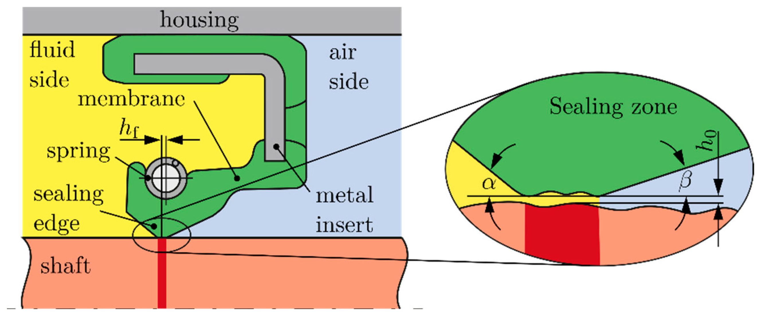
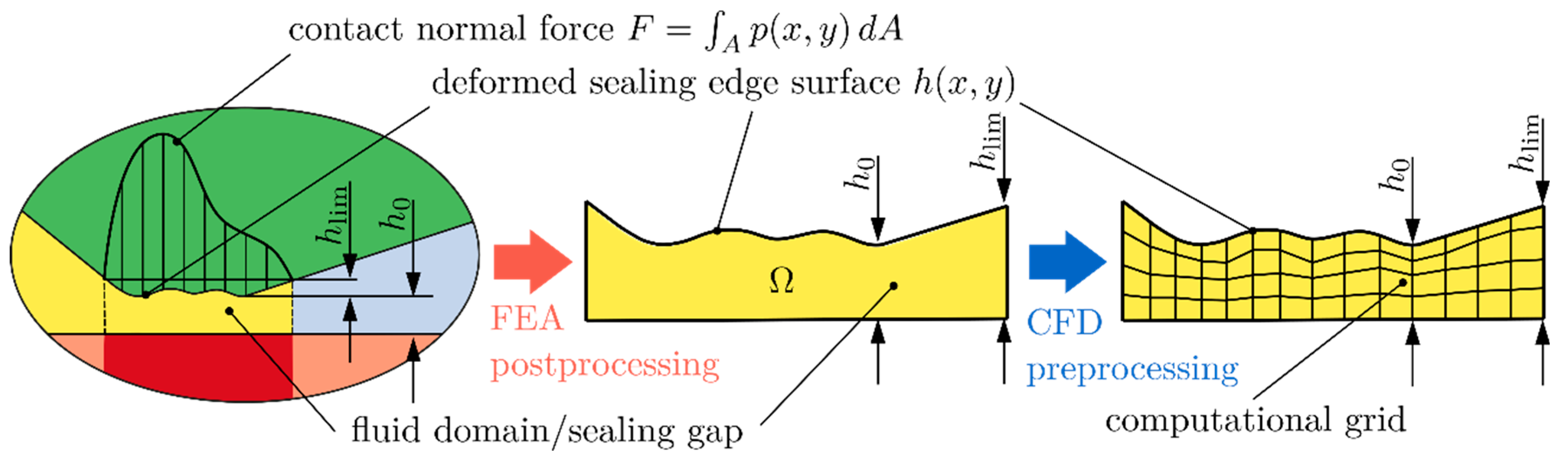
2.2.1. Geometry
2.2.2. Fluid Properties
2.2.3. Geometric and Structural Parameters
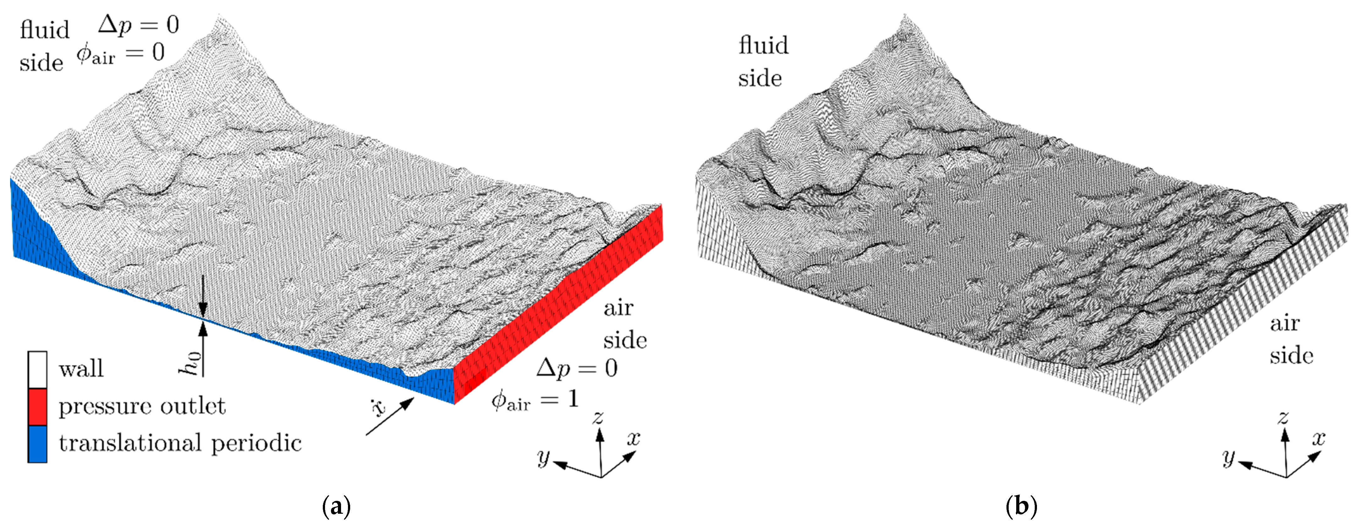
2.2.4. Discretization of the Computational Domain and Boundary Conditions
2.3. Solver Settings and Solution Control
3. Results
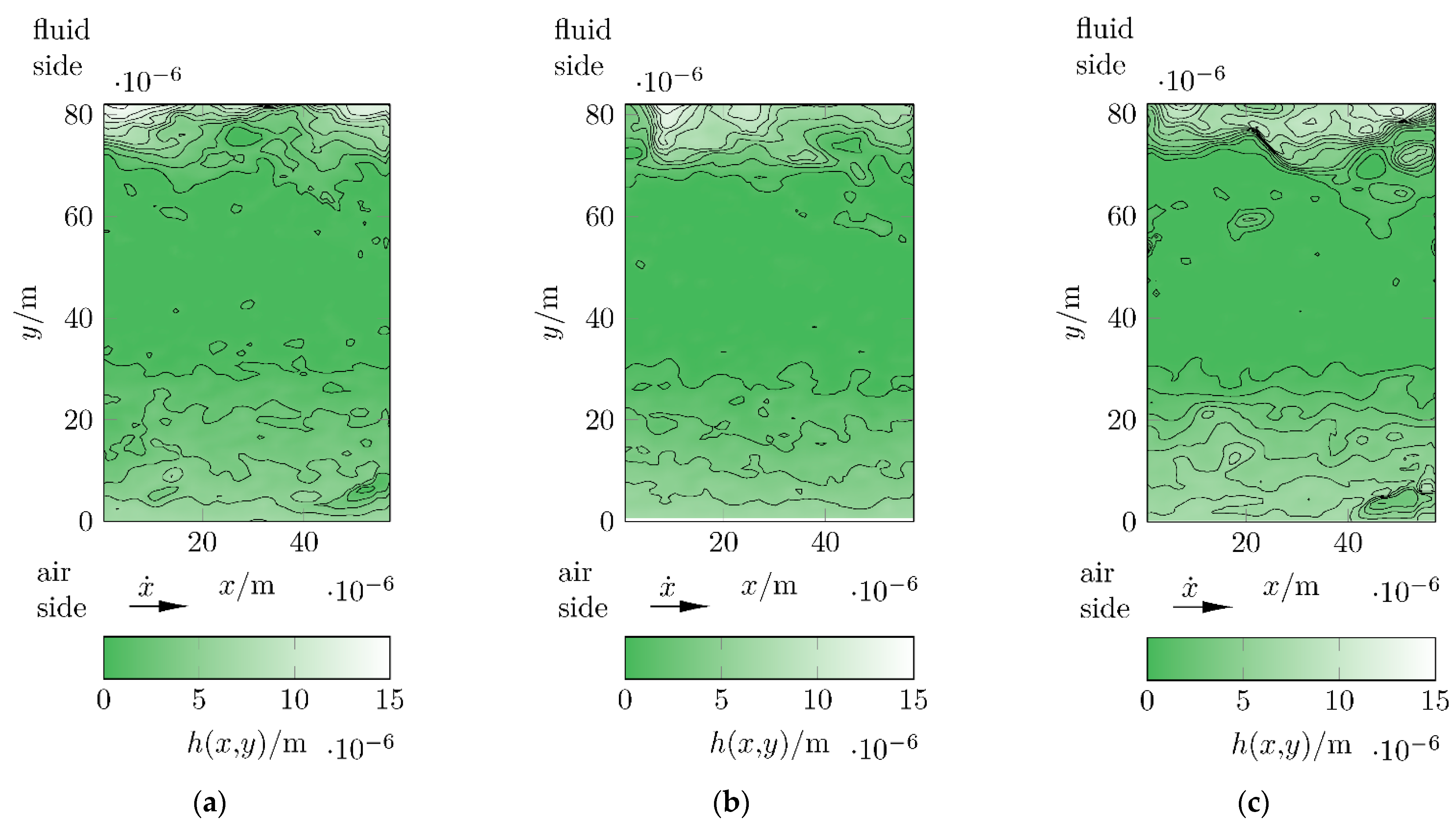
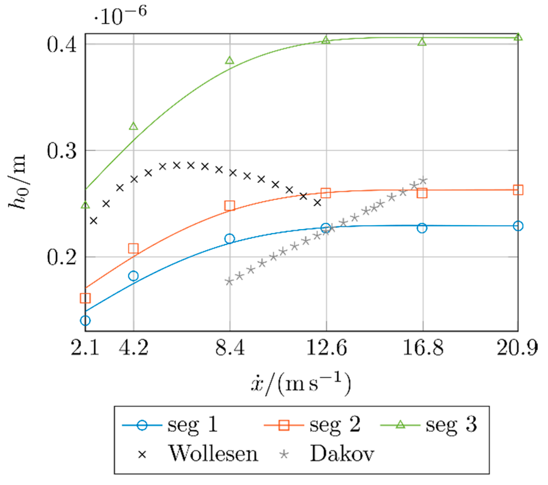
3.1. Sealing Gap Heights
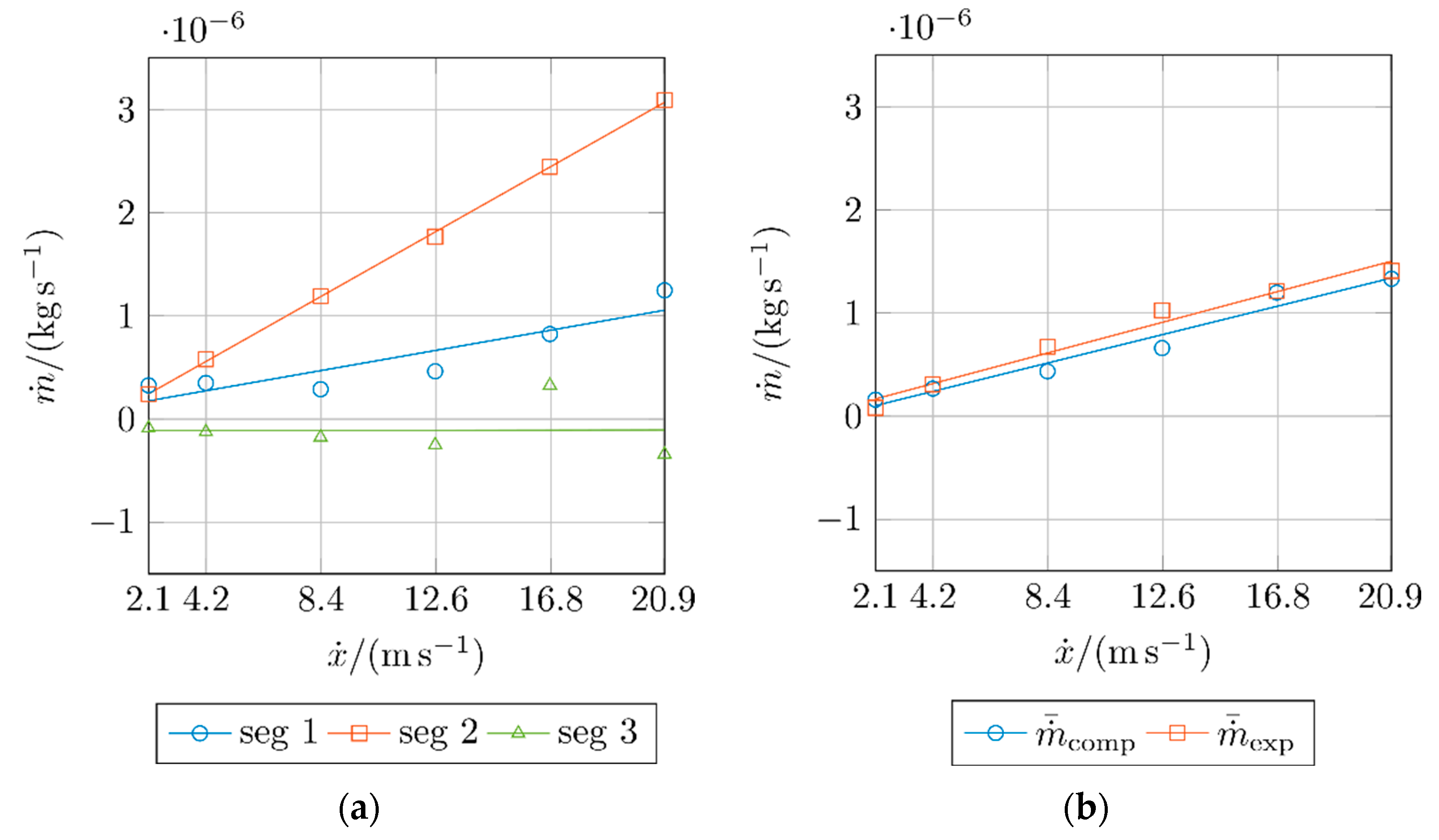
3.2. Pumping Rates
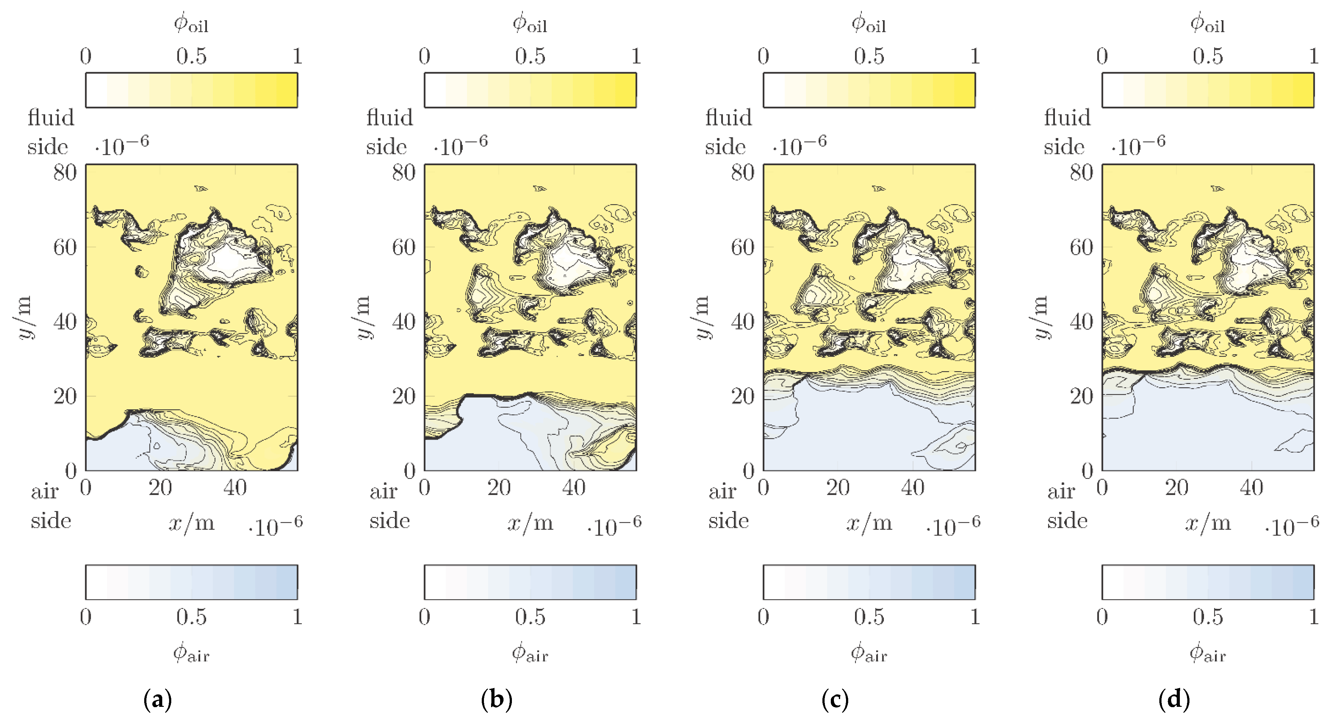
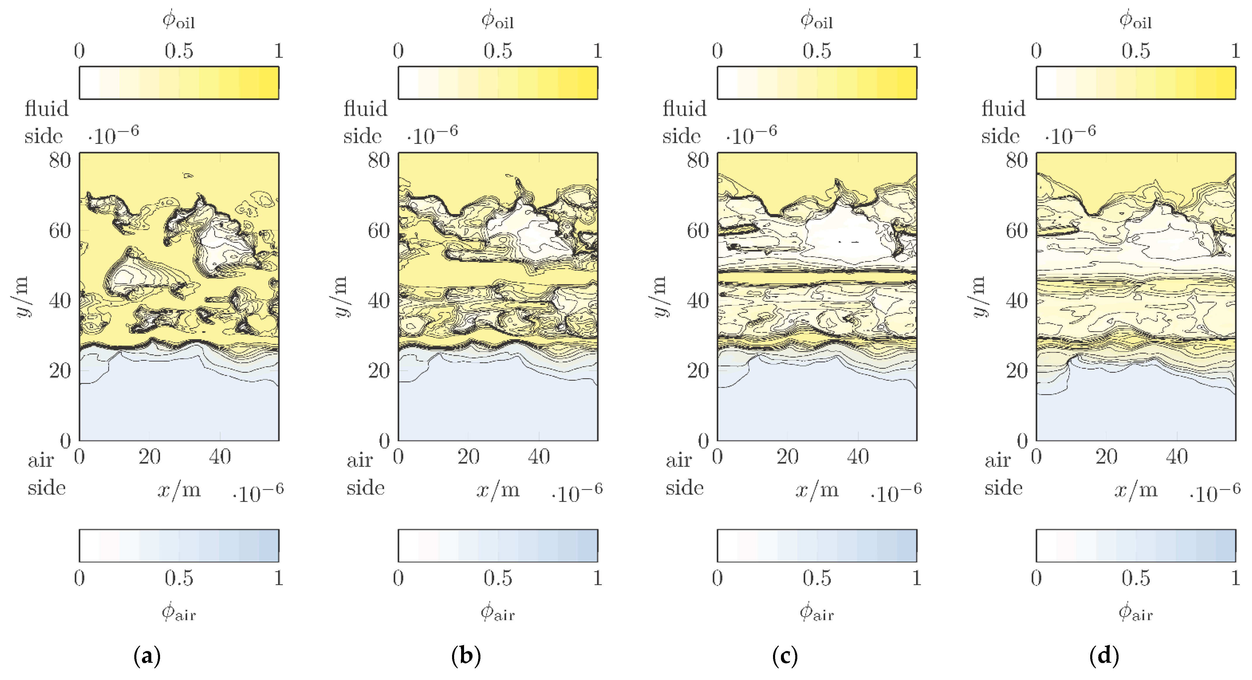
3.3. Phase Interactions and Flow Features
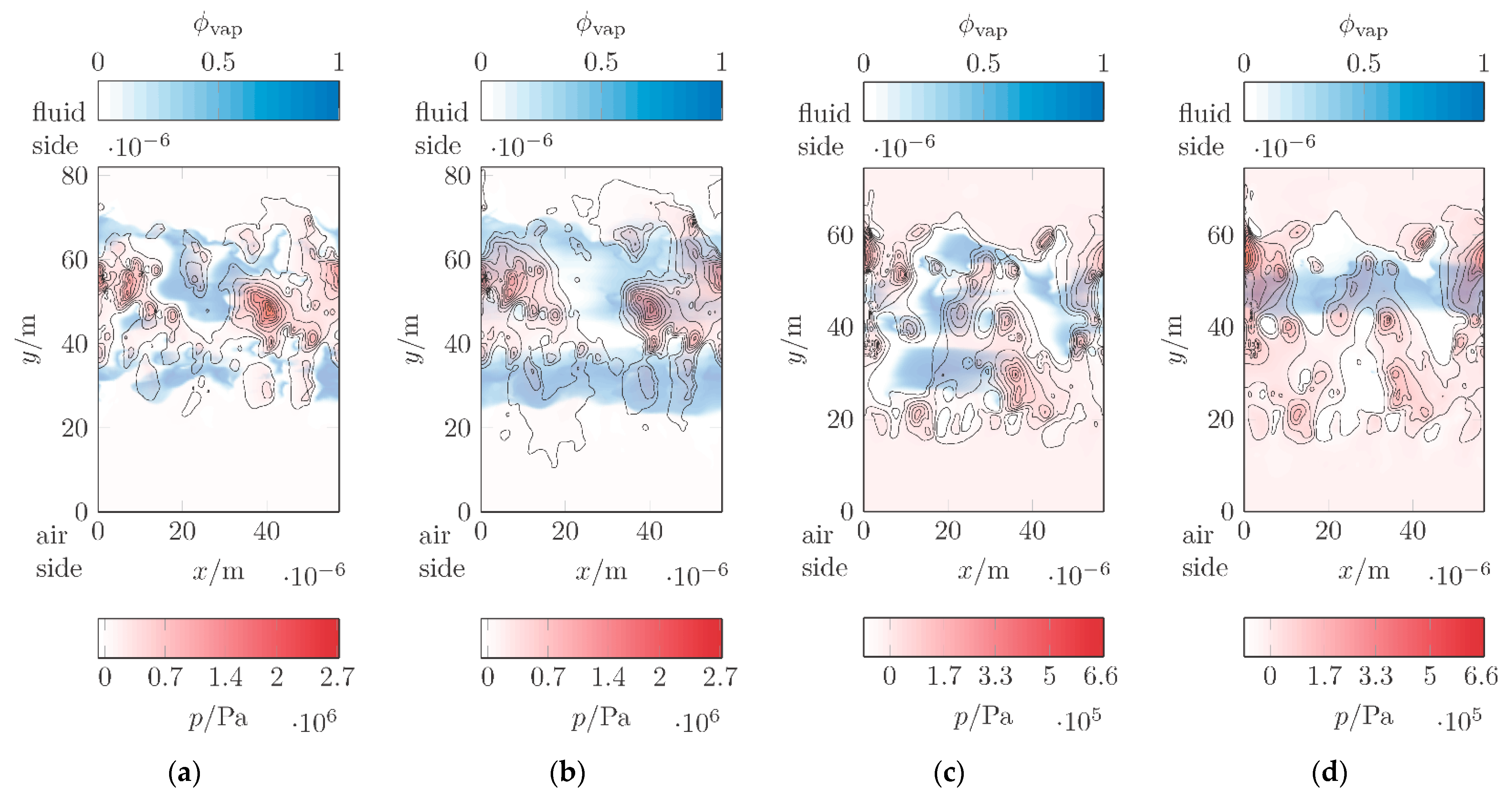
3.4. Cavitation and Hydrodynamic Pressure
4. Conclusions
- Computational fluid dynamics (CFD) is suitable for the computation of transient flow processes of rotary shaft seals.
- The presented method allows the implementation of surface measurement data for this purpose.
- The results of three selected sealing edge segments show different flow processes. This means that the dynamic sealing gap of a rotary shaft seal may not be assumed to be constant but varies over the entire circumference.
- On average, the computed mass flow rates show high agreement with the measured data. Consequently, the presented model provides physically reasonable and valid results.
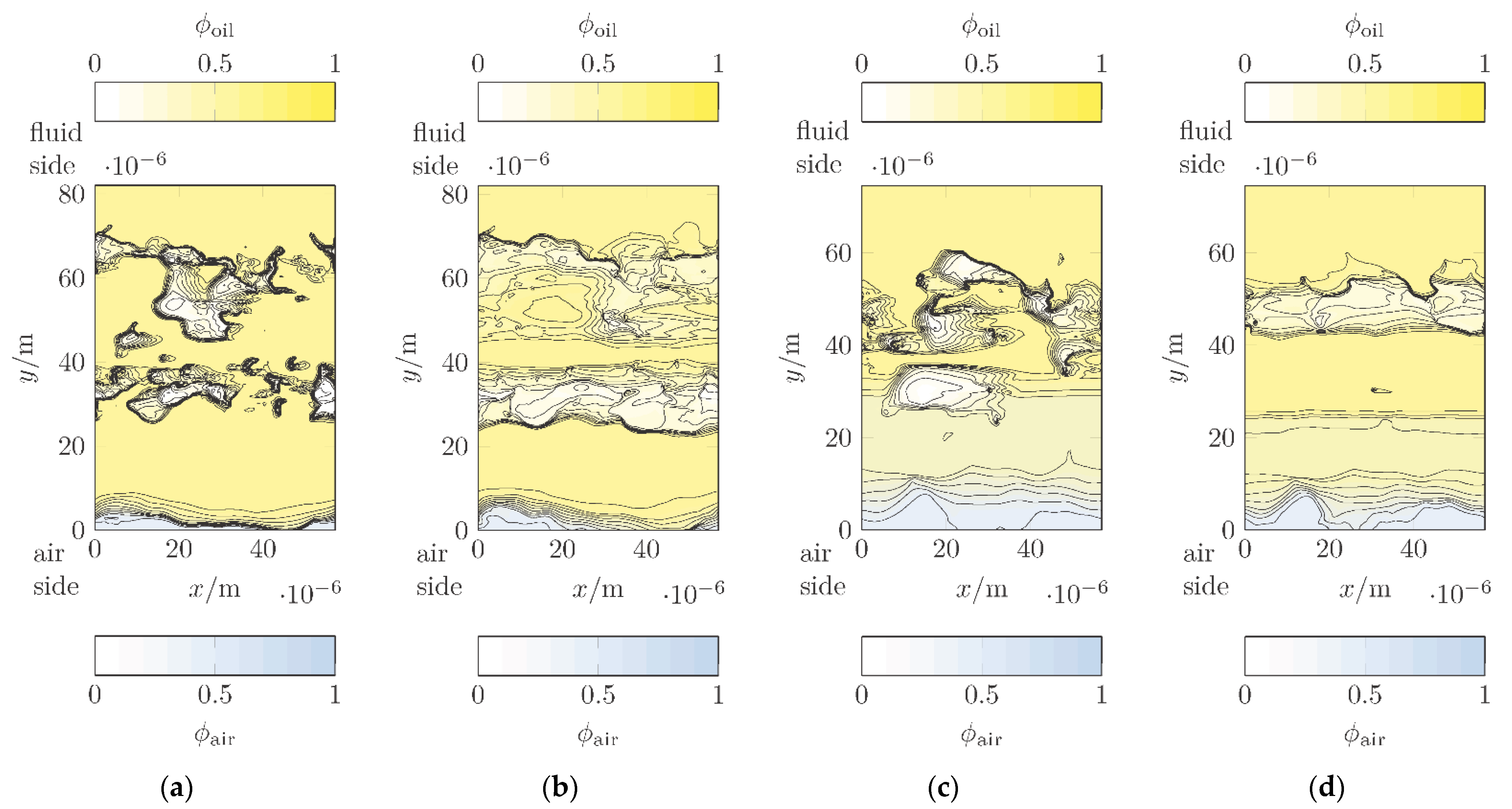
- The computed phase interaction provides an in-depth insight into the sealing and lubrication mechanism of rotary shaft seals. The results show that a steady state is established after a period of . This is in agreement with the results from [7], where at a time of , the motion of the oil meniscus stops and reaches a stable position. A variation of the position of the phase interface depending on the circumferential speed cannot be found.
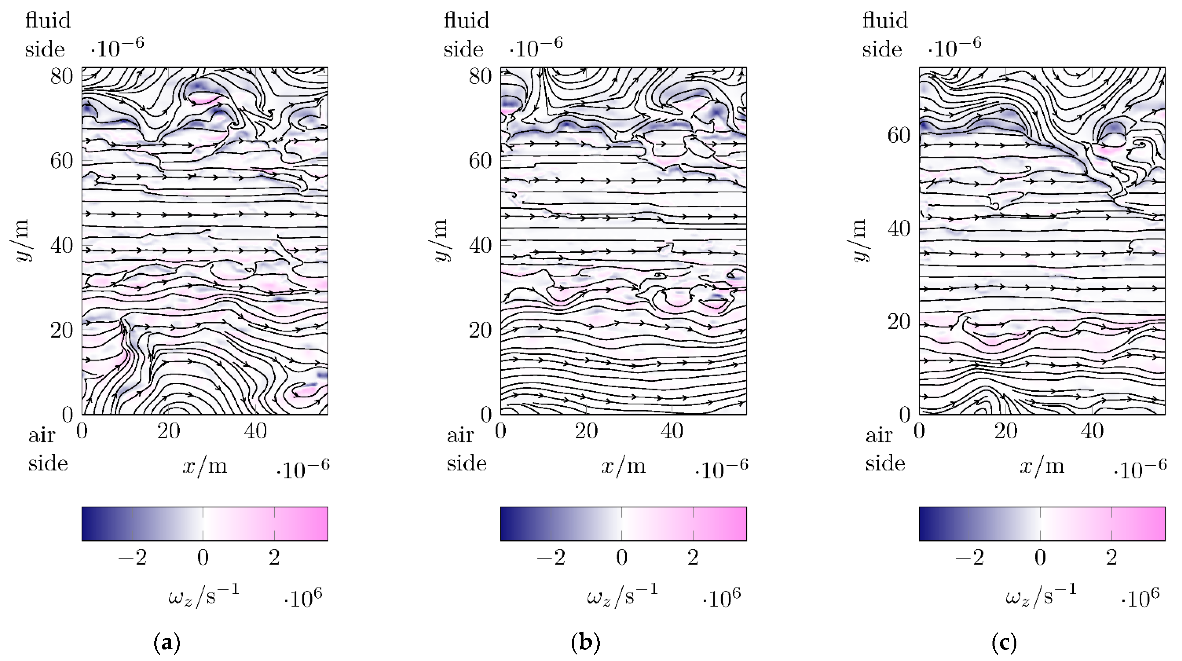
- The flow features show a dominant tangential flow in the lubricant film with axial flow components on the fluid side and on the air side. This provides explanations for the lubrication and sealing mechanism of rotary shaft seals.
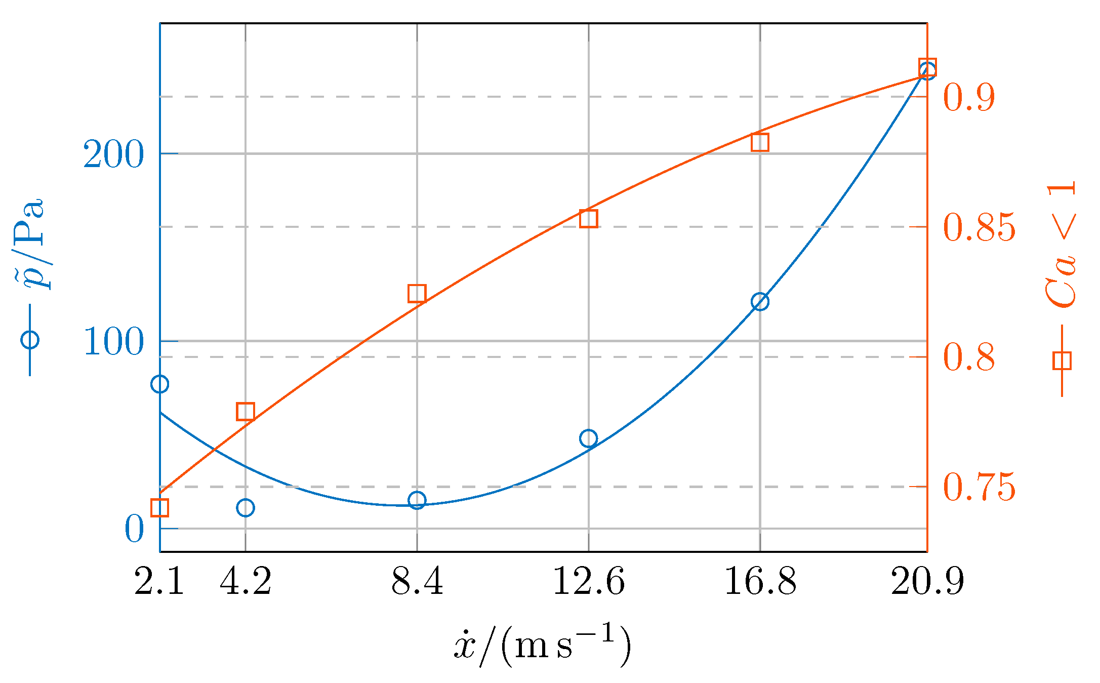
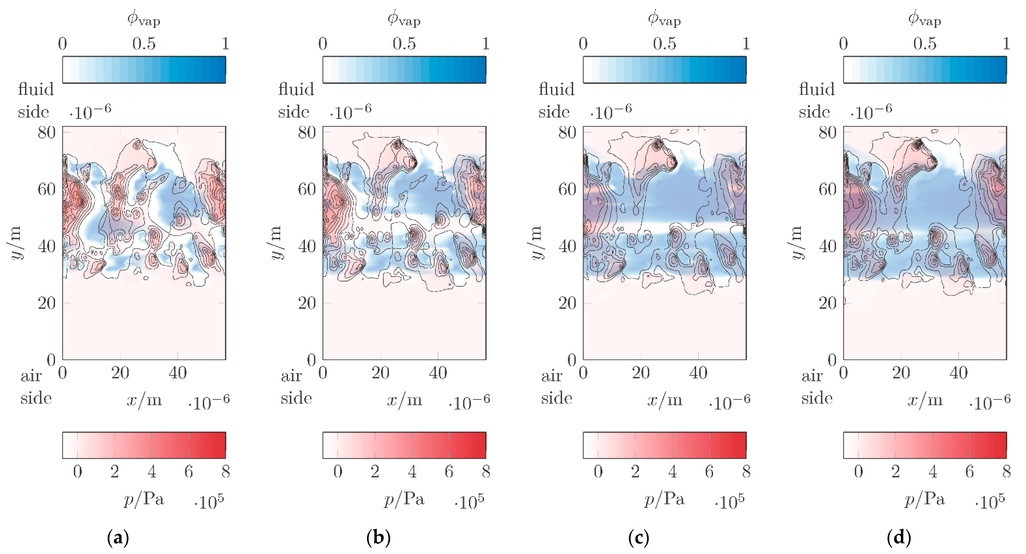
- The analyses of the hydrodynamic pressure and cavitation show that there is almost no noticeable variation over time. However, as the circumferential speed increases, the cavitation zone fraction increases and the pressure increases after a slight drop. The obtained cavitation zone fraction corresponds to the values given in [8].
Author Contributions
Funding
Data Availability Statement
Conflicts of Interest
Nomenclature
| Area of the bottom surface of the fluid domain | |
| Cavitation number | |
| Nominal diameter | |
| Reduced Young’s modulus | |
| Young’s modulus of the sealing ring | |
| Young’s modulus of the shaft | |
| Normal force | |
| Body forces | |
| Gravity vector | |
| Central film thickness | |
| Sealing gap height | |
| Minimum gap height | |
| Central film thickness | |
| Spring lever arm | |
| Limit gap height | |
| Minimum film thickness | |
| Moe’s parameter | |
| Moe’s parameter | |
| Mass transfer rate for condensation | |
| Mass transfer rate for evaporation | |
| Mass flow rate on the fluid side | |
| Dimensionless mass flow rate on the fluid side | |
| Rotational speed | |
| Number of cells | |
| Number of time steps | |
| Number of grid points in circumferential direction | |
| Number of grid points in axial direction | |
| Number of cell layers in radial direction | |
| Local pressure | |
| Median pressure | |
| Vaporization pressure | |
| Radius of the vapor bubbles | |
| Reduced radius of curvature in circumferential direction | |
| Reduced radius of curvature in axial direction | |
| Root mean square height | |
| Time | |
| Time step size | |
| Velocity parameter | |
| Effective velocity | |
| Velocity vector of the th phase | |
| Mass-averaged velocity vector of the mixture | |
| Drift velocity vector | |
| Velocity vector of the vapor phase | |
| Load parameter | |
| ISO distance | |
| Circumferential direction | |
| Circumferential speed | |
| Axial direction | |
| Radial direction | |
| Fluid side contact surface angle | |
| Under-relaxation factor for body forces | |
| Under-relaxation factor for momentum | |
| Under-relaxation factor for pressure | |
| Pressure viscosity coefficient | |
| Under-relaxation factor for vaporization mass | |
| Under-relaxation factor for vaporization mass | |
| Under-relaxation factor for density | |
| Under-relaxation factor for vaporization mass | |
| Air side contact surface angle | |
| Residual criterion of air volume fraction | |
| Residual criterion of continuity | |
| Residual criterion of vapor volume fraction | |
| Residual criterion of circumferential velocity | |
| Residual criterion of axial velocity | |
| Residual criterion of radial velocity | |
| Viscosity of the th phase | |
| Dynamic viscosity of the liquid phase | |
| Viscosity of the mixture | |
| Contact temperature | |
| Oil sump temperature | |
| Effective wavelength in circumferential direction | |
| Effective wavelength in axial direction | |
| Poisson’s ratio of the shaft | |
| Poisson’s ratio of the sealing ring | |
| Local density | |
| Bubble number density | |
| Density of the th phase | |
| Density of the liquid phase | |
| Density of the mixture | |
| Density of the vapor phase | |
| Root mean square slope in circumferential direction | |
| Root mean square slope in axial direction | |
| Volume fraction of the air phase | |
| Volume fraction of the th phase | |
| Volume fraction of the oil phase | |
| Volume fraction of the vapor phase | |
| -vorticity |
Abbreviations
| CFD | Computational fluid dynamics |
| FEA | Grid convergence index |
| GCI | Finite element analyses |
| JFO | Jakobsson–Floberg–Olsson cavitation model |
| UDF | User-defined functions |
References
- DIN 3760:1996-09; Radial-Wellendichtringe. DIN: Berlin, Germany, 1996.
- ISO 6194-1:2007-09; Rotary Shaft Lip-Type Seals Incorporating Elastomeric Sealing Elements—Part 1: Nominal Dimensions and Tolerances. ISO: Geneva, Switzerland, 2007.
- Bauer, F. Federvorgespannte-Elastomer-Radial-Wellendichtungen; Springer Fachmedien Wiesbaden: Wiesbaden, Germany, 2021; ISBN 978-3-658-32921-1. [Google Scholar]
- Bauer, F. Tribologie; Springer Fachmedien Wiesbaden: Wiesbaden, Germany, 2021; ISBN 978-3-658-32919-8. [Google Scholar]
- Kammüller, M. Zur Abdichtwirkung von Radial-Wellendichtringen; Universität Stuttgart: Stuttgart, Germany, 1986. [Google Scholar]
- Müller, H.K. Concepts of Sealing Mechanism of Rubber Lip Type Rotary Shaft Seals. In Proceedings of the 11th International Conference on Fluid Sealing, Cannes, France, 8–10 April 1987; pp. 698–709. [Google Scholar]
- Salant, R.F. Analysis of the Transient Behavior of Rotary Lip Seals-Fluid Mechanics and Bulk Deformation. Tribol. Trans. 1998, 41, 471–480. [Google Scholar] [CrossRef]
- Shen, D.; Salant, R.F. A Transient Mixed Lubrication Model of a Rotary Lip Seal with a Rough Shaft. Tribol. Trans. 2006, 49, 621–634. [Google Scholar] [CrossRef]
- Hajjam, M.; Bonneau, D. A Transient Finite Element Cavitation Algorithm with Application to Radial Lip Seals. Tribol. Int. 2007, 40, 1258–1269. [Google Scholar] [CrossRef]
- Jakobsson, B.; Floberg, L. The Finite Journal Bearing Considering Vaporization, (Das Gleitlager von Endlicher Breite Mit Verdampfung); Chalmers Tekniska Högskolas handlingar; Avd. Maskinteknik; Report from the Institute of Machine Elements, Chalmers University of Technology; Gumpert: Göteborg, Sweden, 1957; Volume 190. [Google Scholar]
- Olsson, K.-O. Cavitation in Dynamically Loaded Bearings; Chalmers Tekniska Högskolas handlingar; Gumperts: Göteborg, Sweden, 1965; Volume 34. [Google Scholar]
- Almqvist, T.; Larsson, R. Some Remarks on the Validity of Reynolds Equation in the Modeling of Lubricant Film Flows on the Surface Roughness Scale. J. Tribol. 2004, 126, 703–710. [Google Scholar] [CrossRef]
- Dobrica, M.B.; Fillon, M. About the Validity of Reynolds Equation and Inertia Effects in Textured Sliders of Infinite Width. Proc. Inst. Mech. Eng. Part J J. Eng. Tribol. 2009, 223, 69–78. [Google Scholar] [CrossRef]
- Yang, A.-S.; Wen, C.-Y.; Tseng, C.-S. Analysis of Flow Field around a Ribbed Helix Lip Seal. Tribol. Int. 2009, 42, 649–656. [Google Scholar] [CrossRef]
- Keller, D.; Jacobs, G.; Neumann, S. Development of a Low-Friction Radial Shaft Seal: Using CFD Simulations to Optimise the Microstructured Sealing Lip. Lubricants 2020, 8, 41. [Google Scholar] [CrossRef] [Green Version]
- Ungarish, M. Hydrodynamics of Suspensions: Fundamentals of Centrifugal and Gravity Separation; Springer: Berlin, Germany; New York, NY, USA, 1993; ISBN 978-3-540-54762-4. [Google Scholar]
- Gidaspow, D. Multiphase Flow and Fluidization: Continuum and Kinetic Theory Descriptions; Academic Press: Boston, MA, USA, 1994; ISBN 978-0-12-282470-8. [Google Scholar]
- Hamilton, D.B.; Walowit, J.A.; Allen, C.M. A Theory of Lubrication by Microirregularities. J. Basic Eng. 1966, 88, 177–185. [Google Scholar] [CrossRef]
- Schnerr, G.H.; Sauer, J. Physical and Numerical Modeling of Unsteady Cavitation Dynamics; ICMF New Orleans: New Orleans, LO, USA, 2001; p. 12. [Google Scholar]
- Grün, J.; Feldmeth, S.; Bauer, F. Wear on Radial Lip Seals: A Numerical Study of the Influence on the Sealing Mechanism. Wear 2021, 476, 203674. [Google Scholar] [CrossRef]
- Grün, J.; Feldmeth, S.; Bauer, F. The Sealing Mechanism of Radial Lip Seals: A Numerical Study of the Tangential Distortion of the Sealing Edge. Tribol. Mater. 2022, 1, 1–10. [Google Scholar] [CrossRef]
- Marx, N.; Guegan, J.; Spikes, H.A. Elastohydrodynamic Film Thickness of Soft EHL Contacts Using Optical Interferometry. Tribol. Int. 2016, 99, 267–277. [Google Scholar] [CrossRef] [Green Version]
- Sperka, P.; Krupka, I.; Hartl, M. Analytical Formula for the Ratio of Central to Minimum Film Thickness in a Circular EHL Contact. Lubricants 2018, 6, 80. [Google Scholar] [CrossRef] [Green Version]
- Hamrock, B.J.; Brewe, D. Simplified Solution for Stresses and Deformations. J. Lubr. Technol. 1983, 105, 171–177. [Google Scholar] [CrossRef]
- Dowson, D.; Higginson, G.R. The Effect of Material Properties on the Lubrication of Elastic Rollers. J. Mech. Eng. Sci. 1960, 2, 188–194. [Google Scholar] [CrossRef]
- Dowson, D.; Higginson, G.R.; Whitaker, A.V. Elasto-Hydrodynamic Lubrication: A Survey of Isothermal Solutions. J. Mech. Eng. Sci. 1962, 4, 121–126. [Google Scholar] [CrossRef]
- Karami, G.; Evans, H.P.; Snidle, R.W. Elastohydrodynamic Lubrication of Circumferentially Finished Rollers Having Sinusoidal Roughness. Proc. Inst. Mech. Eng. Part C J. Mech. Eng. Sci. 1987, 201, 29–36. [Google Scholar] [CrossRef]
- Griffiths, B. Manufacturing Surface Technology; Elsevier: Amsterdam, The Netherlands, 2001; ISBN 978-1-85718-029-9. [Google Scholar]
- Moes, H. Communications. In Proceedings of the Symposium on Elastohydrodynamic Lubrication, London, UK, 21–23 September 1965; Volume 180, pp. 244–245. [Google Scholar]
- Feldmeth, S.; Bauer, F.; Haas, W. Abschätzung der Kontakttemperatur bei Radial-Wellendichtungen mit der Selbstentwickelten Open-Source-Software InsECT. In Proceedings of the KISSsoft AG (Hg.) 2016—Tagungsband Schweizer Maschinenelemente Kolloquium SMK, Stuttgart, Germany, 12–13 October 2016; pp. 233–248. [Google Scholar]
- Grün, J.; Feldmeth, S.; Bauer, F. Computational Fluid Dynamics of the Lubricant Flow in the Sealing Gap of Rotary Shaft Seals. In Proceedings of the M2D2022—9th International Conference on Mechanics and Materials in Design, Funchal, Portugal, 26–30 June 2022; pp. 1035–1050. [Google Scholar]
- Forschungsvereinigung Antriebstechnik, e.V. Referenzöle Für Wälz-und Gleitlager-, Zahnrad-und Kupplungsversuche; Forschungsvereinigung Antriebstechnik e.V.: Hesse, Germany, 1985; Volume 180. [Google Scholar]
- Biswas, R.; Strawn, R.C. Tetrahedral and Hexahedral Mesh Adaptation for CFD Problems. Appl. Numer. Math. 1998, 26, 135–151. [Google Scholar] [CrossRef]
- Gao, R.; Kirk, G. CFD Study on Stepped and Drum Balance Labyrinth Seal. Tribol. Trans. 2013, 56, 663–671. [Google Scholar] [CrossRef]
- Adjemout, M.; Brunetiere, N.; Bouyer, J. Optimization of Mesh Density for Numerical Simulations of Hydrodynamic Lubrication Considering Textured Surfaces. Proc. Inst. Mech. Eng. Part J J. Eng. Tribol. 2015, 229, 1132–1144. [Google Scholar] [CrossRef]
- Snyder, T.; Braun, M. Comparison of Perturbed Reynolds Equation and CFD Models for the Prediction of Dynamic Coefficients of Sliding Bearings. Lubricants 2018, 6, 5. [Google Scholar] [CrossRef]
- Roache, P.J. Perspective: A Method for Uniform Reporting of Grid Refinement Studies. J. Fluids Eng. 1994, 116, 405–413. [Google Scholar] [CrossRef]
- Celik, I.B.; Ghia, U.; Roache, P.J.; Freitas, C.J.; Coleman, H.; Raad, P.E. Procedure for Estimation and Reporting of Uncertainty Due to Discretization in CFD Applications. J. Fluids Eng. 2008, 130, 078001. [Google Scholar] [CrossRef] [Green Version]
- Patankar, S.V.; Spalding, D.B. A Calculation Procedure for Heat, Mass and Momentum Transfer in Three-Dimensional Parabolic Flows. Int. J. Heat Mass Transf. 1972, 15, 1787–1806. [Google Scholar] [CrossRef]
- Wollesen, V. Temperaturbestimmung in der Dichtzone von Radialwellendichtringen als Randbedingung für die Modellierung des Dichtvorganges; Technische Universität Hamburg-Harburg: Hamburg, Germany, 1993. [Google Scholar]
- Dakov, N. Elastohydrodynamic Lubrication Analysis of a Radial Oil Seal with Hydrodynamic Features. Tribol. Int. 2022, 173, 107653. [Google Scholar] [CrossRef]
- Merkle, L.; Baumann, M.; Bauer, F. Back-Pumping Rate Measurement of Elastomeric Radial Lip Seals in Converse Installation: Basics, Wear Formation and Long-Term Tests. In Proceedings of the M2D2022—9th International Conference on MECHANICS and Materials in Design, Funchal, Portugal, 26–30 June 2022; pp. 363–374. [Google Scholar]
- Galletti, C.; Mariotti, A.; Siconolfi, L.; Mauri, R.; Brunazzi, E. Numerical Investigation of Flow Regimes in T-Shaped Micromixers: Benchmark between Finite Volume and Spectral Element Methods. Can. J. Chem. Eng. 2019, 97, 528–541. [Google Scholar] [CrossRef]
- Batchelor, G.K. An Introduction to Fluid Dynamics, 1st ed.; Cambridge University Press: New York, NY, USA, 2000; ISBN 978-0-521-66396-0. [Google Scholar]
- Arndt, R.E.A. Cavitation in Fluid Machinery and Hydraulic Structures. Annu. Rev. Fluid Mech. 1981, 13, 273–326. [Google Scholar] [CrossRef]
- Brennen, C.E. Cavitation and Bubble Dynamics; Cambridge University Press: New York, NY, USA, 2014; ISBN 978-1-107-64476-2. [Google Scholar]


| Rotational Speed | Circumferential Speed | Contact Temperature | Dynamic Viscosity | Pressure Viscosity Coefficient | Density |
|---|---|---|---|---|---|
| 500 | 2.1 | 82.4 | 0.0147 | 836 | |
| 1000 | 4.2 | 89.6 | 0.0118 | 830 | |
| 2000 | 8.4 | 103.8 | 0.0081 | 824 | |
| 3000 | 12.6 | 117.3 | 0.0059 | 812 | |
| 4000 | 16.8 | 130.2 | 0.0044 | 806 | |
| 5000 | 20.9 | 142.5 | 0.0036 | 800 |
| Fluid | Dynamic Viscosity | Density |
|---|---|---|
| lubricant vapor | 1.2 | |
| air | 1.225 |
| Segment | Root Mean Square Height | Root Mean Square Slope | Root Mean Square Slope | Effective Wave Length | Effective Wave Length | Reduced Radius of Curvature | Reduced Radius of Curvature |
|---|---|---|---|---|---|---|---|
| seg 1 | |||||||
| seg 2 | |||||||
| seg 3 |
| Number of Grid Points | Number of Grid Points | Number of Cell Layers | Number of Cells | GCI |
|---|---|---|---|---|
| 140 | 200 | 3 | 82,983 | - |
| 280 | 400 | 6 | 667,926 | |
| 420 | 600 | 9 | 2,258,829 | |
| 560 | 800 | 12 | 5,359,692 |
| Under-Relaxation Factor | Symbol | Value |
|---|---|---|
| pressure | ||
| density | 1.0 | |
| body forces | 1.0 | |
| momentum | 0.3 | |
| vaporization mass | 1.0 | |
| slip velocity | 0.1 | |
| volume fraction | 0.5 |
Publisher’s Note: MDPI stays neutral with regard to jurisdictional claims in published maps and institutional affiliations. |
© 2022 by the authors. Licensee MDPI, Basel, Switzerland. This article is an open access article distributed under the terms and conditions of the Creative Commons Attribution (CC BY) license (https://creativecommons.org/licenses/by/4.0/).
Share and Cite
Grün, J.; Feldmeth, S.; Bauer, F. Multiphase Computational Fluid Dynamics of Rotary Shaft Seals. Lubricants 2022, 10, 347. https://doi.org/10.3390/lubricants10120347
Grün J, Feldmeth S, Bauer F. Multiphase Computational Fluid Dynamics of Rotary Shaft Seals. Lubricants. 2022; 10(12):347. https://doi.org/10.3390/lubricants10120347
Chicago/Turabian StyleGrün, Jeremias, Simon Feldmeth, and Frank Bauer. 2022. "Multiphase Computational Fluid Dynamics of Rotary Shaft Seals" Lubricants 10, no. 12: 347. https://doi.org/10.3390/lubricants10120347