
Accurate Segmentation of Nuclear Regions with Multi-Organ Histopathology Images Using Artificial Intelligence for Cancer Diagnosis in Personalized Medicine

 ,
,  , , and
Abstract
:
1. Introduction
- -
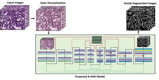
- In our proposed method, full-size patches of 1000 × 1000 pixels for TCGA dataset and 512 × 512 pixels for the TNBC dataset are processed without converting them into sub-patches, whereas existing methods converts full-size patches into sub-patches before performing segmentation. The proposed method exhibited good segmentation performance without the additional requirements of sub-patch conversion. In addition, our method does not require postprocessing, unlike other nuclear segmentation techniques.
- -
- The performance of nuclear segmentation is improved by maintaining high-frequency information owing to spatial information transfer from the encoder to the decoder through residual connectivity.
- -
- With the specified design, we reduce the number of convolution layers, and the proposed R-SNN utilizes fewer trainable parameters.
- -
- The training of the network is fast, and the network converges rapidly in only 30 epochs (27,210 iterations) on average, owing to the residual connections and reduced structure of the network.
- -
- As shown in [18], our trained models and codes are available on request for research purposes.
2. Related Works
2.1. Handcrafted-Feature-Based Methods
2.2. Deep-Feature-Based Methods
3. Proposed Method
3.1. Overview of the Proposed Architecture
3.2. Preprocessing by Stain Normalization
3.3. Architecture of the Proposed R-SNN
3.4. Loss Function
4. Experiments and Performance Analysis
4.1. Datasets
4.1.1. TCGA Dataset
4.1.2. TNBC Dataset
4.2. Data Augmentation
4.3. Experimental Setup and Training
4.3.1. Experimental Setup
4.3.2. Training
4.4. Performance Evaluation of the Proposed Method
4.4.1. Performance Evaluation Metric
4.4.2. Ablation Study
4.4.3. Comparisons with State-of-the-Art Methods
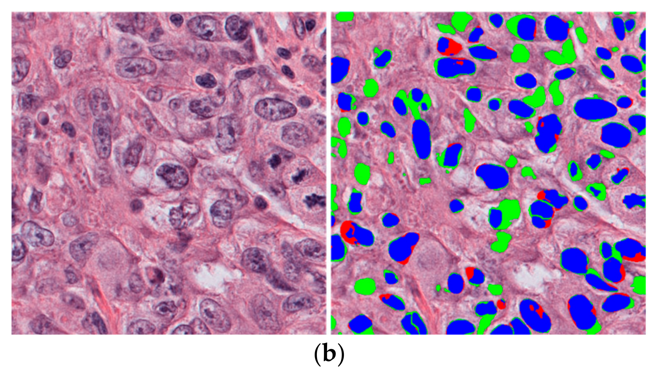
4.4.4. Correct and Incorrect Detection Cases Using the Proposed Method
5. Discussion
- Stain normalization plays a key role in the classification, detection, and segmentation of histopathology images because it removes the inconsistencies caused by the staining and environmental factors. The performance of deep-learning models was also improved, as presented in Table 6, where the experiments performed with stain normalization showed higher accuracy than those without stain normalization.
- Shallow networks lack generalization capabilities; therefore, deep networks are mostly developed. However, in the case of applications related to histopathology images, a severe vanishing gradient problem mostly occurs because the ROIs are usually tiny and, thus, may vanish due to successive convolution operations. In our proposed technique, we confined the feature map size to 31 × 31, which positively influenced the performance of our segmentation model. The performance of SegNet was lower than that of the proposed technique because the final feature map size of the encoder was 7 × 7 in SegNet, indicating that important information may be lost in successive convolution operations.
- The residual skip connections from the encoder to the decoder of the proposed R-SNN empowered feature representation, which enabled the network to perform well despite having only a few layers of convolution. In the proposed technique, only 10 convolution layers were used in the encoder. However, the proposed model showed higher accuracy than the state-of-the-art models because the residual skip connections retained important information helpful for nuclear segmentation.
- AI-based applications can be applied to digital pathology because of their good generalization capabilities, high performance, and short inference time. Experiments on two datasets—TCGA dataset containing images from breast, kidney, liver, prostate, bladder, colon, stomach, lung, and brain, and the TNBC dataset containing breast cancer images—proved that AI-based applications have a good generalization capability.
- Accurate, robust, and computationally inexpensive AI-based methods play a very important role in boosting the confidence level of pathologists toward AI. In this regard, the proposed method can be adopted for real-time applications owing to its good performance, robustness, and low computational cost.
- Despite the above, our proposed work had a few limitations. First, an intensive task of stain normalization was performed, which could cause high computational complexity. Second, neighboring nuclei were difficult to separate and were considered a single object. Third, many applications involve whole-slide images, which are much larger than 1000 × 1000 pixels. The extension of our research to whole-slide image processing across different magnifications is required as future work.
6. Conclusions
Author Contributions
Funding
Institutional Review Board Statement
Informed Consent Statement
Data Availability Statement
Acknowledgments
Conflicts of Interest
References
- Chow, K.-H.; Factor, R.E.; Ullman, K.S. The nuclear envelope environment and its cancer connections. Nat. Rev. Cancer 2012, 12, 196–209. [Google Scholar] [CrossRef] [PubMed] [Green Version]
- Pan, X.; Lu, Y.; Lan, R.; Liu, Z.; Qin, Z.; Wang, H.; Liu, Z. Mitosis detection techniques in H&E stained breast cancer pathological images: A comprehensive review. Comput. Electr. Eng. 2021, 91, 1–17. [Google Scholar]
- Filipczuk, P.; Fevens, T.; Krzyzak, A.; Monczak, R. Computer-aided breast cancer diagnosis based on the analysis of cytological images of fine needle biopsies. IEEE Trans. Med. Imaging 2013, 32, 2169–2178. [Google Scholar] [CrossRef] [PubMed]
- Chang, H.; Han, J.; Borowsky, A.; Loss, L.; Gray, J.W.; Spellman, P.T.; Parvin, B. Invariant delineation of nuclear architecture in glioblastoma multiforme for clinical and molecular association. IEEE Trans. Med. Imaging 2013, 32, 670–682. [Google Scholar] [CrossRef]
- Kumar, N.; Verma, R.; Arora, A.; Kumar, A.; Gupta, S.; Sethi, A.; Gann, P.H. Convolutional neural networks for prostate cancer recurrence prediction. In Proceedings of the Medical Imaging 2017: Digital Pathology, Orlando, FL, USA, 1 March 2017; International Society for Optics and Photonics: Bellingham, Was, USA, 2017; Volume 10140, p. 101400. [Google Scholar]
- Zhao, M.; Wang, H.; Han, Y.; Wang, X.; Dai, H.N.; Sun, X.; Zhang, J.; Pedersen, M. Seens: Nuclei segmentation in pap smear images with selective edge enhancement. Futur. Gener. Comp. Syst. 2021, 114, 185–194. [Google Scholar] [CrossRef]
- Gharipour, A.; Liew, A.W. Segmentation of cell nuclei in fluorescence microscopy images: An integrated framework using levelset segmentation and touching-cell splitting. Pattern Recognit. 2016, 58, 185–194. [Google Scholar] [CrossRef]
- George, Y.M.; Bagoury, B.M.; Zayed, H.H.; Roushdy, M.I. Automated cell nuclei segmentation for breast fine needle aspiration cytology. Signal Process. 2013, 93, 2804–2816. [Google Scholar] [CrossRef]
- Bentaieb, A.; Hamarneh, G. Adversarial stain transfer for histopathology image analysis. IEEE Trans. on Med. Imaging 2018, 37, 792–802. [Google Scholar] [CrossRef] [PubMed]
- Ullah, A.; Muhammad, K.; Ding, W.; Palade, V.; Haq, I.U.; Baik, S.W. Efficient activity recognition using lightweight CNN and DS-GRU network for surveillance applications. Appl. Soft. Comput. 2021, 103, 107102. [Google Scholar] [CrossRef]
- Nguyen, M.H.; Nguyen, D.L.; Nguyen, X.M.; Quan, T.T. Auto-detection of sophisticated malware using lazy-binding control flow graph and deep learning. Comput. Secur. 2018, 76, 128–155. [Google Scholar] [CrossRef]
- Shuvo, S.B.; Ali, S.N.; Swapnil, S.I.; Al-Rakhami, M.S.; Gumaei, A. CardioXNet: A novel lightweight deep learning framework for cardiovascular disease classification using heart sound recordings. IEEE Access 2021, 9, 36955–36967. [Google Scholar] [CrossRef]
- Sheikh, T.S.; Lee, Y.; Cho, M. Histopathological classification of breast cancer images using a multi-scale input and multi-feature network. Cancers 2020, 12, 2031. [Google Scholar] [CrossRef] [PubMed]
- Fu, Y.; Jung, A.W.; Torne, R.V.; Gonzalez, S.; Vöhringer, H.; Shmatko, A.; Yates, L.R.; Jimenez-Linan, M.; Moore, L.; Gerstung, M. Pan-Cancer Computational Histopathology Reveals Mutations, Tumor Composition and Prognosis. Nat. Cancer 2020, 1, 800–810. [Google Scholar] [CrossRef]
- Otsu, N. A Threshold Selection Method from Gray-Level Histograms. IEEE Trans. Syst. Man Cybern. 1979, 9, 62–66. [Google Scholar] [CrossRef] [Green Version]
- Vincent, L.; Soille, P. Watersheds in Digital Spaces: An Efficient Algorithm Based on Immersion Simulations. IEEE Trans. Pattern Anal. Mach. Intell. 1991, 13, 583–598. [Google Scholar] [CrossRef] [Green Version]
- Chenyang, X.; Prince, J.L. Snakes, Shapes, and Gradient Vector Flow. IEEE Trans. Image Process. 1998, 7, 359–369. [Google Scholar] [CrossRef] [Green Version]
- Nuclei-Net Model with Algorithms. Available online: http://dm.dgu.edu/link.html (accessed on 10 August 2020).
- Bartels, P.H.; Weber, J.E.; Duckstein, L. Machine Learning in Quantitative Histopathology. Anal. Quant. Cytol. Histol. 1988, 10, 299–306. [Google Scholar]
- Huang, P.-W.; Lai, Y.-H. Effective Segmentation and Classification for HCC Biopsy Images. Pattern Recognit. 2010, 43, 1550–1563. [Google Scholar] [CrossRef]
- Yang, X.; Li, H.; Zhou, X. Nuclei Segmentation Using Marker-Controlled Watershed, Tracking Using Mean-Shift, and Kalman Filter in Time-Lapse Microscopy. IEEE Trans. Circuits Syst. I Regul. Pap. 2006, 53, 2405–2414. [Google Scholar] [CrossRef]
- Cosatto, E.; Miller, M.; Graf, H.P.; Meyer, J.S. Grading Nuclear Pleomorphism on Histological Micrographs. In Proceedings of the 2008 19th International Conference on Pattern Recognition, Tampa, FL, USA, 8–11 December 2008; pp. 1–4. [Google Scholar]
- Illingworth, J.; Kittler, J. The Adaptive Hough Transform. IEEE Trans. Pattern Anal. Mach. Intell. 1987, 9, 690–698. [Google Scholar] [CrossRef] [PubMed]
- Ali, S.; Madabhushi, A. An integrated region-, boundary-, shape-based active contour for multiple object overlap resolution in histological imagery. IEEE Trans. Med. Imaging 2012, 31, 1448–1460. [Google Scholar] [CrossRef]
- Kong, H.; Gurcan, M.; Belkacem-Boussaid, K. Partitioning Histopathological Images: An Integrated Framework for Supervised Color-Texture Segmentation and Cell Splitting. IEEE Trans. Med. Imaging 2011, 30, 1661–1677. [Google Scholar] [CrossRef] [PubMed] [Green Version]
- Plissiti, M.E.; Nikou, C. Overlapping Cell Nuclei Segmentation Using a Spatially Adaptive Active Physical Model. IEEE Trans. Image Process. 2012, 21, 4568–4580. [Google Scholar] [CrossRef]
- Vuola, A.O.; Akram, S.U.; Kannala, J. Mask-RCNN and U-Net Ensembled for Nuclei Segmentation. In Proceedings of the 2019 IEEE 16th International Symposium on Biomedical Imaging (ISBI 2019), Venice, Italy, 8–11 April 2019; pp. 208–212. [Google Scholar]
- Johnson, J.W. Adapting Mask-RCNN for Automatic Nucleus Segmentation. arXiv 2020, arXiv:1805.00500. [Google Scholar]
- Kumar, N.; Verma, R.; Sharma, S.; Bhargava, S.; Vahadane, A.; Sethi, A. A Dataset and a Technique for Generalized Nuclear Segmentation for Computational Pathology. IEEE Trans. Med. Imaging 2017, 36, 1550–1560. [Google Scholar] [CrossRef]
- Carpenter, A.E.; Jones, T.R.; Lamprecht, M.R.; Clarke, C.; Kang, I.H.; Friman, O.; Guertin, D.A.; Chang, J.H.; Lindquist, R.A.; Moffat, J.; et al. CellProfiler: Image Analysis Software for Identifying and Quantifying Cell Phenotypes. Genome Biol. 2006, 7, R100. [Google Scholar] [CrossRef] [Green Version]
- Schindelin, J.; Arganda-Carreras, I.; Frise, E.; Kaynig, V.; Longair, M.; Pietzsch, T.; Preibisch, S.; Rueden, C.; Saalfeld, S.; Schmid, B.; et al. Fiji: An Open-Source Platform for Biological-Image Analysis. Nat. Methods 2012, 9, 676–682. [Google Scholar] [CrossRef] [PubMed] [Green Version]
- Naylor, P.; Laé, M.; Reyal, F.; Walter, T. Nuclei Segmentation in Histopathology Images Using Deep Neural Networks. In Proceedings of the 2017 IEEE 14th International Symposium on Biomedical Imaging (ISBI 2017), Melbourne, Australia, 18–21 April 2017; pp. 933–936. [Google Scholar]
- Pang, B.; Zhang, Y.; Chen, Q.; Gao, Z.; Peng, Q.; You, X. Cell Nucleus Segmentation in Color Histopathological Imagery Using Convolutional Networks. In Proceedings of the 2010 Chinese Conference on Pattern Recognition (CCPR), Chongqing, China, 21–23 October 2010; pp. 1–5. [Google Scholar]
- Long, J.; Shelhamer, E.; Darrell, T. Fully Convolutional Networks for Semantic Segmentation. In Proceedings of the IEEE Conference on Computer Vision and Pattern Recognition (CVPR), Boston, MA, USA, 7–12 June 2015; pp. 3431–3440. [Google Scholar]
- Noh, H.; Hong, S.; Han, B. Learning Deconvolution Network for Semantic Segmentation. In Proceedings of the IEEE International Conference on Computer Vision (ICCV), Santiago, Chile, 7–13 December 2015; pp. 1520–1528. [Google Scholar]
- Kang, Q.; Lao, Q.; Fevens, T. Nuclei Segmentation in Histopathological Images Using Two-Stage Learning. In Proceedings of the Medical Image Computing and Computer Assisted Intervention—MICCAI 2019, Shenzhen, China, 13–17 October 2019; Shen, D., Liu, T., Peters, T.M., Staib, L.H., Essert, C., Zhou, S., Yap, P.-T., Khan, A., Eds.; Springer International Publishing: Cham, Switzerland, 2019; pp. 703–711. [Google Scholar]
- Zhou, Y.; Onder, O.F.; Dou, Q.; Tsougenis, E.; Chen, H.; Heng, P.-A. CIA-Net: Robust Nuclei Instance Segmentation with Contour-Aware Information Aggregation. In Proceedings of the Information Processing in Medical Imaging, Ambleside, UK, 20–25 July 2003; Chung, A.C.S., Gee, J.C., Yushkevich, P.A., Bao, S., Eds.; Springer International Publishing: Cham, Switzerland, 2019; pp. 682–693. [Google Scholar]
- Mahbod, A.; Schaefer, G.; Ellinger, I.; Ecker, R.; Smedby, Ö.; Wang, C. A Two-Stage U-Net Algorithm for Segmentation of Nuclei in H&E-Stained Tissues. In Proceedings of the Digital Pathology, Warwick, UK, 10–13 April 2019; Reyes-Aldasoro, C.C., Janowczyk, A., Veta, M., Bankhead, P., Sirinukunwattana, K., Eds.; Springer International Publishing: Cham, Switzerland, 2019; pp. 75–82. [Google Scholar]
- Zeng, Z.; Xie, W.; Zhang, Y.; Lu, Y. RIC-Unet: An Improved Neural Network Based on Unet for Nuclei Segmentation in Histology Images. IEEE Access 2019, 7, 21420–21428. [Google Scholar] [CrossRef]
- Chidester, B.; Ton, T.-V.; Tran, M.-T.; Ma, J.; Do, M.N. Enhanced Rotation-Equivariant U-Net for Nuclear Segmentation. In Proceedings of the 2019 IEEE/CVF Conference on Computer Vision and Pattern Recognition Workshops (CVPRW), Long Beach, CA, USA, 16–17 June 2019; pp. 1097–1104. [Google Scholar]
- Anghel, A.; Stanisavljevic, M.; Andani, S.; Papandreou, N.; Rüschoff, J.H.; Wild, P.; Gabrani, M.; Pozidis, H. A High-Performance System for Robust Stain Normalization of Whole-Slide Images in Histopathology. Front. Med. 2019, 6. [Google Scholar] [CrossRef]
- Arsalan, M.; Kim, D.S.; Owais, M.; Park, K.R. OR-Skip-Net: Outer Residual Skip Network for Skin Segmentation in Non-Ideal Situations. Expert Syst. Appl. 2020, 141, 112922. [Google Scholar] [CrossRef]
- Macenko, M.; Niethammer, M.; Marron, J.S.; Borland, D.; Woosley, J.T.; Xiaojun, G.; Schmitt, C.; Thomas, N.E. A Method for Normalizing Histology Slides for Quantitative Analysis. In Proceedings of the 2009 IEEE International Symposium on Biomedical Imaging: From Nano to Macro, Boston, MA, USA, 28 June–1 July 2009; IEEE: Piscataway, NJ, USA, 2009; pp. 1107–1110. [Google Scholar]
- He, K.; Zhang, X.; Ren, S.; Sun, J. Deep Residual Learning for Image Recognition. In Proceedings of the 2016 IEEE Conference on Computer Vision and Pattern Recognition (CVPR), Las Vegas, NV, USA, 27–30 June 2016; IEEE: Piscataway, NJ, USA, 2016; pp. 770–778. [Google Scholar]
- Sudre, C.H.; Li, W.; Vercauteren, T.; Ourselin, S.; Jorge Cardoso, M. Generalised Dice Overlap as a Deep Learning Loss Function for Highly Unbalanced Segmentations. In Proceedings of the Deep Learning in Medical Image Analysis and Multimodal Learning for Clinical Decision Support, Québec City, QC, Canada, 14 September 2017; Cardoso, M.J., Arbel, T., Carneiro, G., Syeda-Mahmood, T., Tavares, J.M.R.S., Moradi, M., Bradley, A., Greenspan, H., Papa, J.P., Madabhushi, A., et al., Eds.; Springer International Publishing: Cham, Switzerland, 2017; pp. 240–248. [Google Scholar]
- Yun, P.; Tai, L.; Wang, Y.; Liu, C.; Liu, M. Focal Loss in 3D Object Detection. IEEE Robot. Autom. Lett. 2019, 4, 1263–1270. [Google Scholar] [CrossRef] [Green Version]
- Bach, S.H.; Broecheler, M.; Huang, B.; Getoor, L. Hinge-Loss Markov Random Fields and Probabilistic Soft Logic. J. Mach. Learn. Res. 2017, 18, 3846–3912. [Google Scholar]
- Ho, Y.; Wookey, S. The Real-World-Weight Cross-Entropy Loss Function: Modeling the Costs of Mislabeling. IEEE Access 2020, 8, 4806–4813. [Google Scholar] [CrossRef]
- Tomczak, K.; Czerwińska, P.; Wiznerowicz, M. The Cancer Genome Atlas (TCGA): An Immeasurable Source of Knowledge. Contemp. Oncol. 2015, 19, A68–A77. [Google Scholar] [CrossRef]
- Kumar, N.; Verma, R.; Anand, D.; Zhou, Y.; Onder, O.F.; Tsougenis, E.; Chen, H.; Heng, P.-A.; Li, J.; Hu, Z.; et al. A Multi-Organ Nucleus Segmentation Challenge. IEEE Trans. Med. Imaging 2020, 39, 1380–1391. [Google Scholar] [CrossRef]
- Agarwal, G.; Nanda, G.; Lal, P.; Mishra, A.; Agarwal, A.; Agrawal, V.; Krishnani, N. Outcomes of Triple-Negative Breast Cancers (TNBC) Compared with Non-TNBC: Does the Survival Vary for All Stages? World J. Surg. 2016, 40, 1362–1372. [Google Scholar] [CrossRef] [PubMed]
- MATLAB R2019a at a Glance. Available online: https://www.mathworks.com/products/new_products/release2019a.html (accessed on 10 February 2021).
- Intel Core i7-7700 Processor. Available online: https://www.intel.com/content/www/us/en/products/processors/core/i7-processors/i7-7700.html (accessed on 10 February 2021).
- GeForce GTX 1070. Available online: https://www.nvidia.com/ko-kr/geforce/products/10series/geforce-gtx-1070-ti/ (accessed on 10 February 2021).
- Melinte, D.O.; Vladareanu, L. Facial Expressions Recognition for Human–Robot Interaction Using Deep Convolutional Neural Networks with Rectified Adam Optimizer. Sensors 2020, 20, 2393. [Google Scholar] [CrossRef]
- Weerdt, J.D.; Backer, M.D.; Vanthienen, J.; Baesens, B. A Robust F-measure for Evaluating Discovered Process Models. In Proceedings of the 2011 IEEE Symposium on Computational Intelligence and Data Mining, Paris, France, 11–15 April 2011; pp. 1–8. [Google Scholar]
- Dice, L.R. Measures of the Amount of Ecologic Association Between Species. Ecology 1945, 26, 297–302. [Google Scholar] [CrossRef]
- Yu, F.; Wang, D.; Shelhamer, E.; Darrell, T. Deep Layer Aggregation. In Proceedings of the 2018 IEEE/CVF Conference on Computer Vision and Pattern Recognition, Salt Lake City, UT, USA, 18–23 June 2018; IEEE: Piscataway, NJ, USA, 2018; pp. 2403–2412. [Google Scholar]
- Ronneberger, O.; Fischer, P.; Brox, T. U-Net: Convolutional Networks for Biomedical Image Segmentation. In Proceedings of the Medical Image Computing and Computer-Assisted Intervention—MICCAI 2015, Munich, Germany, 5–9 October 2015; Navab, N., Hornegger, J., Wells, W.M., Frangi, A.F., Eds.; Springer International Publishing: Cham, Switzerland, 2015; pp. 234–241. [Google Scholar]
- He, K.; Gkioxari, G.; Dollár, P.; Girshick, R.B. Mask R-CNN. In Proceedings of the 2017 IEEE International Conference on Computer Vision (ICCV), Venice, Italy, 22–29 October 2017. [Google Scholar] [CrossRef]
- Selvaraju, R.R.; Cogswell, M.; Das, A.; Vedantam, R.; Parikh, D.; Batra, D. Grad-CAM: Visual Explanations From Deep Networks via Gradient-Based Localization. In Proceedings of the 2017 IEEE International Conference on Computer Vision (ICCV), Venice, Italy, 22–29 October 2017; pp. 618–626. [Google Scholar]


| Type | Techniques | Strength | Weakness |
|---|---|---|---|
| Handcrafted feature-based | Marker-controlled watershed segmentation, and combination of mean shift and the Kalman filter for the tracking of nuclei [21] | Superior performance to other techniques such as k-means clustering | -Long inference time -Optimization of marking region is required. |
| Segmentation based on the Hough transform and active model [22] | -Robust to noisy data -Can handle missing information -Can easily adapt to different shapes | -Computationally complex and expensive, and has a low accuracy -Inability to separate connecting objects | |
| Active contour and shape model with the integration of region, boundary, and shape information [24] | Autonomous and self-adaptation can track objects in both temporal and spatial directions | -Need for an initial counter -Can become stuck in local minima -Computationally expensive and has a long runtime -Cannot manage intensity inhomogeneity effectively | |
| Marker-controlled watershed segmentation, snake model, and SVM classifier [20] | -Resulting boundaries of the objects correspond to contours -Postprocessing not required | -Excessive over-segmentation and requires the optimization of marker -Long inference time | |
| Deep feature-based | Mask-RCNN [28] | Good for instance segmentation | High computational cost of region proposals |
| Three-class CNN [29] | Simple structure | Uses many parameters due to fully connected layers | |
| PangNet, FCN, DeconvNet, and ensemble classification [32] | Good for jointly segmented nuclei | Postprocessing overhead and low accuracy | |
| Two-stage learning using U-Net and DLA [36] | High accuracy by considering nuclear segmentation as a three-class problem | Computationally expensive due to two stages and multiple networks | |
| Multilevel information aggregation using task-specific decoders and novel smooth truncated loss [37] | Good generalization capability because the network focuses on learning from reliable and informative samples | Computationally expensive due to multiple decoder networks | |
| U-Net-based classification and regression in two sequential stages [38] | -Good performance for the prediction of the pixels of the border -Images of different sizes can be used as input due to the absence of a dense layer in U-Net | Postprocessing overhead and requires many learnable parameters | |
| U-Net variant [39] | -Inception module captures detailed information | Postprocessing overhead | |
| U-Net variant with group-equivariant convolution and upsampling [40] | -Easy training on multiple GPUs and possibility of model parallelization -Can learn powerful representations based on symmetry pattern | -Postprocessing overhead and requires many learnable parameters -Low performance due to the lack of meaningful relationships based on relative positions, orientations, and scales | |
| R-SNN (the proposed method) | Robust segmentation with fewer trainable parameters without postprocessing | Stain normalization as preprocessing |
| Block | Name/Size | Number of Filters | Output Feature Map Size (Width × Height × Number of Channels) | Number of Trainable Parameters |
|---|---|---|---|---|
| EB-1 | EConvBR-1_1/3 × 3 × 3 To decoder (RC-1) | 64 | 500 × 500 × 64 | 1792 + 128 |
| EConvBR-1_2/3 × 3 × 64 | 64 | 36,928 + 128 | ||
| Pooling-1 | Pool-1/2 × 2 | - | 250 × 250 × 64 | - |
| EB-2 | EConvBR-2_1/3 × 3 × 64 To decoder (RC-2) | 128 | 250 × 250 × 128 | 73,856 + 256 |
| EConBR-2_2/3 × 3 × 128 | 128 | 147,584 + 256 | ||
| Pooling-2 | Pool-2/2 × 2 | - | 125 × 125 × 128 | - |
| EB-3 | EConvBR-3_1/3 × 3 × 128 To decoder (RC-3) | 256 | 125 × 125 × 256 | 295,168 + 512 |
| EConvBR-3_2/3 × 3 × 256 | 256 | 590,080 + 512 | ||
| EConvBR-3_3/3 × 3 × 256 | 256 | 590,080 + 512 | ||
| Pooling-3 | Pool-3/2×2 | - | 62 × 62 × 256 | - |
| EB-4 | EConvBR-4_1/3 × 3 × 256 To decoder (RC-4) | 512 | 62 × 62 × 512 | 1,180,160 + 1024 |
| EConvBR-4_2/3 × 3 × 512 | 512 | 2,359,808 + 1024 | ||
| EConvBR-4_3/3 × 3 × 512 | 512 | 2,359,808 + 1024 | ||
| Pooling-4 | Pool-4/2 × 2 | - | 31 × 31 × 512 | - |
| Unpooling-4 | Unpool-4 | - | 62 × 62 × 512 | - |
| DB-4 | DConvBR-4_3/3 × 3 × 512 | 512 | 2,359,808 + 1024 | |
| DConvBR-4_2/3 × 3 × 512 | 512 | 2,359,808 + 1024 | ||
| Add-4 (DConvBR-4_2 + RC-4) | - | - | ||
| DConvBR-4_1/3 × 3 × 512 | 256 | 62 × 62 × 256 | 1,179,904 + 512 | |
| Unpooling-3 | Unpool-3 | - | 125 × 125 × 256 | - |
| DB-3 | DConvBR-3_3/3 × 3 × 256 | 256 | 590,080 + 512 | |
| DConvBR-3_2/3 × 3 × 256 | 256 | 590,080 + 512 | ||
| Add-3 (DConvBR-3_2 + RC-3) | - | - | ||
| DConvBR-3_1/3 × 3 × 256 | 128 | 125 × 125 × 128 | 295040 + 256 | |
| Unpooling-2 | Unpool-2 | - | 250 × 250 × 128 | - |
| DB-2 | DConvBR-2_2/3 × 3 × 128 | 128 | 147,584 + 256 | |
| Add-2 (DConvBR-2_2 + RC-2) | - | - | ||
| DConvBR-2_1/3 × 3 × 128 | 64 | 250 × 250 × 64 | 73,792 + 128 | |
| Unpooling-1 | Unpool-1 | - | 500 × 500 × 64 | - |
| DB-1 | DConvBR-1_2/3 × 3 × 64 | 64 | 36,928 + 128 | |
| Add-1 (DConvBR-1_2 + RC-1) | - | - | ||
| Output | DConvBR-1_1/3 × 3 × 64 | 2 | 500 × 500 × 2 | 1154 + 4 |
| Data | Organ | |||||||||
|---|---|---|---|---|---|---|---|---|---|---|
| Total | Breast | Kidney | Liver | Prostate | Bladder | Colon | Stomach | Lung | Brain | |
| Training | 30 | 6 | 6 | 6 | 6 | 2 | 2 | 2 | - | - |
| Testing | 14 | 2 | 3 | - | 2 | 2 | 1 | - | 2 | 2 |
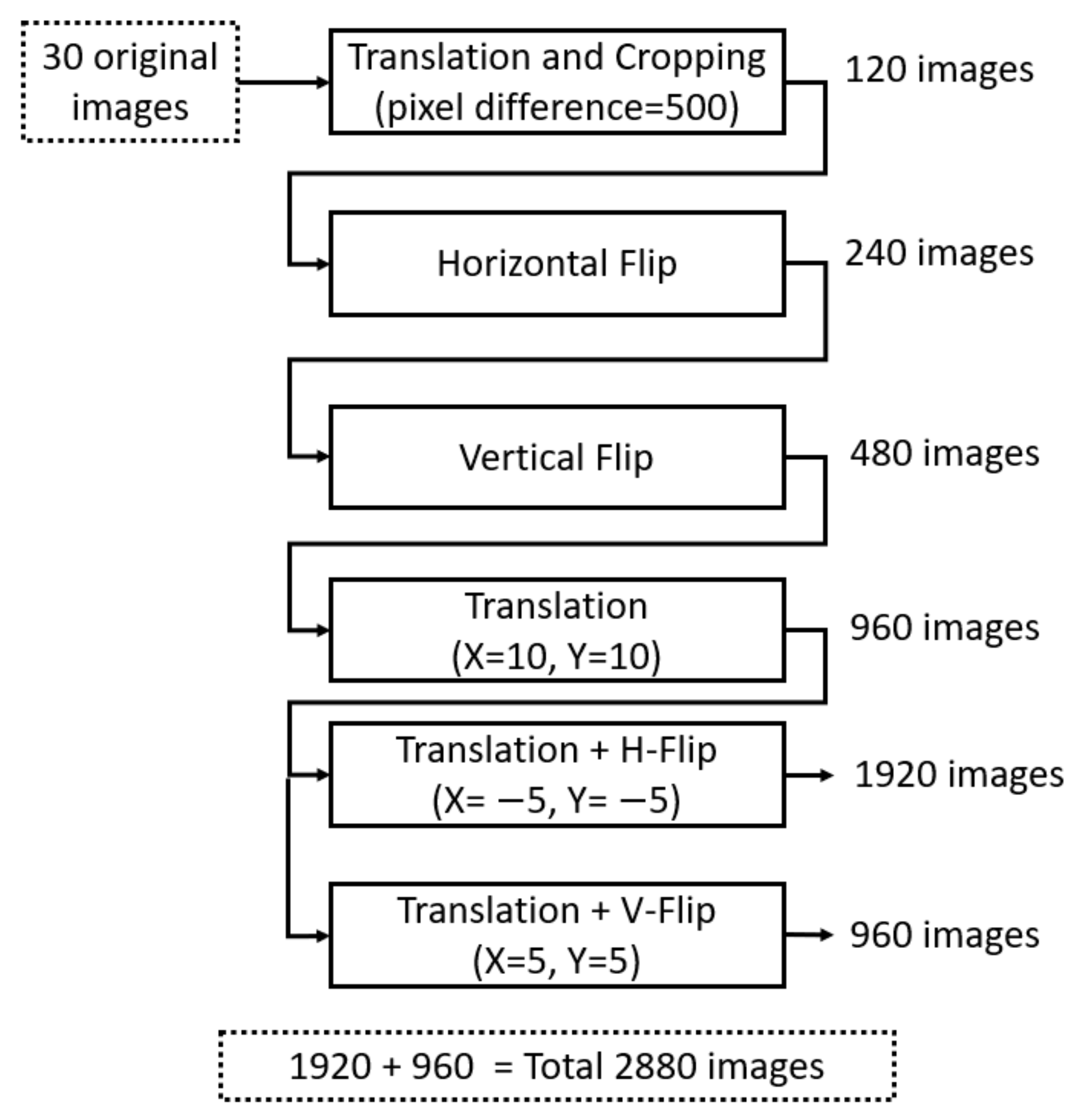
| Dataset | Original Images | Data Augmentation | Total | |||
|---|---|---|---|---|---|---|
| Translation and Cropping | Horizontal Flipping | Vertical Flipping | Translation, Cropping, and Resizing | |||
| TCGA | 30 | 120 | 120 | 240 | 2400 | 2880 |
| TNBC | 43 | 172 | 172 | 344 | 1376 | 2064 |
| Methods | AJI | DC | F1-Measure |
|---|---|---|---|
| No data augmentation | 0.5546 | 0.7120 | 0.6845 |
| With data augmentation | 0.6420 | 0.7749 | 0.8165 |
| Methods | AJI | DC | F1-Measure |
|---|---|---|---|
| Without normalization | 0.6420 | 0.7749 | 0.8165 |
| With normalization | 0.6794 | 0.8084 | 0.8547 |
| Technique | AJI | DC | F1-Measure | Number of Parameters |
|---|---|---|---|---|
| Proposed Network (no skip connections) | 0.6540 | 0.7902 | 0.7617 | 29,444,162 |
| Proposed Network-RC (Concatenation) | 0.6704 | 0.8020 | 0.8161 | 29,444,162 |
| Proposed Network-RC (Addition) | 0.6731 | 0.8039 | 0.8274 | 29,444,162 |
| Proposed Network-RL | 0.6738 | 0.8067 | 0.8342 | 15,279,174 |
| Proposed Network-RC + RL | 0.6794 | 0.8084 | 0.8547 | 15,279,174 |
| Size of Input Image | AJI | DC | F1-Measure |
|---|---|---|---|
| 2000 × 2000 | 0.5410 | 0.7004 | 0.5996 |
| 1500 × 1500 | 0.6185 | 0.7633 | 0.7452 |
| 1000 × 1000 | 0.6794 | 0.8084 | 0.8547 |
| 500 × 500 | 0.5955 | 0.7453 | 0.7977 |
| Loss Function | AJI | DC | F1-Measure |
|---|---|---|---|
| Dice loss [45] | 0.6764 | 0.8063 | 0.8475 |
| Focal loss [46] | 0.6726 | 0.8035 | 0.8317 |
| Cross-entropy loss | 0.6794 | 0.8084 | 0.8547 |
| Methods | AJI | DC | F1-Measure |
|---|---|---|---|
| Cell profiler [29,30] | 0.1232 | 0.5974 | 0.4046 |
| Fiji [29,31] | 0.2733 | 0.6493 | 0.6649 |
| Kumar et al. [29] | 0.5083 | 0.7623 | 0.8267 |
| Kang et al. [36] | 0.5895 | – | 0.8079 |
| Zhou et al. [37] | 0.6306 | – | 0.8458 |
| Mahbod et al. [38] | 0.5687 | 0.7939 | 0.8267 |
| Zeng et al. [39] | 0.5635 | 0.8008 | 0.8278 |
| Chidester et al. [40] | 0.6291 | 0.7980 | 0.8490 |
| Proposed method | 0.6794 | 0.8084 | 0.8547 |
| Methods | AJI | DC | Precision | Recall | F1-Measure |
|---|---|---|---|---|---|
| PangNet [32,33] | – | – | 0.814 | 0.655 | 0.676 |
| DeconvNet [32,35] | – | – | 0.864 | 0.773 | 0.805 |
| FCN [32,34] | – | – | 0.823 | 0.752 | 0.763 |
| Ensemble [32] | – | – | 0.741 | 0.900 | 0.802 |
| Kang et al. [36] | 0.611 | 0.826 | 0.833 | 0.829 | |
| Proposed method | 0.7332 | 0.8441 | 0.8352 | 0.8306 | 0.8329 |
Publisher’s Note: MDPI stays neutral with regard to jurisdictional claims in published maps and institutional affiliations. |
© 2021 by the authors. Licensee MDPI, Basel, Switzerland. This article is an open access article distributed under the terms and conditions of the Creative Commons Attribution (CC BY) license (https://creativecommons.org/licenses/by/4.0/).
Share and Cite
Mahmood, T.; Owais, M.; Noh, K.J.; Yoon, H.S.; Koo, J.H.; Haider, A.; Sultan, H.; Park, K.R. Accurate Segmentation of Nuclear Regions with Multi-Organ Histopathology Images Using Artificial Intelligence for Cancer Diagnosis in Personalized Medicine. J. Pers. Med. 2021, 11, 515. https://doi.org/10.3390/jpm11060515
Mahmood T, Owais M, Noh KJ, Yoon HS, Koo JH, Haider A, Sultan H, Park KR. Accurate Segmentation of Nuclear Regions with Multi-Organ Histopathology Images Using Artificial Intelligence for Cancer Diagnosis in Personalized Medicine. Journal of Personalized Medicine. 2021; 11(6):515. https://doi.org/10.3390/jpm11060515
Chicago/Turabian StyleMahmood, Tahir, Muhammad Owais, Kyoung Jun Noh, Hyo Sik Yoon, Ja Hyung Koo, Adnan Haider, Haseeb Sultan, and Kang Ryoung Park. 2021. "Accurate Segmentation of Nuclear Regions with Multi-Organ Histopathology Images Using Artificial Intelligence for Cancer Diagnosis in Personalized Medicine" Journal of Personalized Medicine 11, no. 6: 515. https://doi.org/10.3390/jpm11060515