
Artificial Intelligence-Based Recognition of Different Types of Shoulder Implants in X-ray Scans Based on Dense Residual Ensemble-Network for Personalized Medicine


Abstract
:1. Introduction
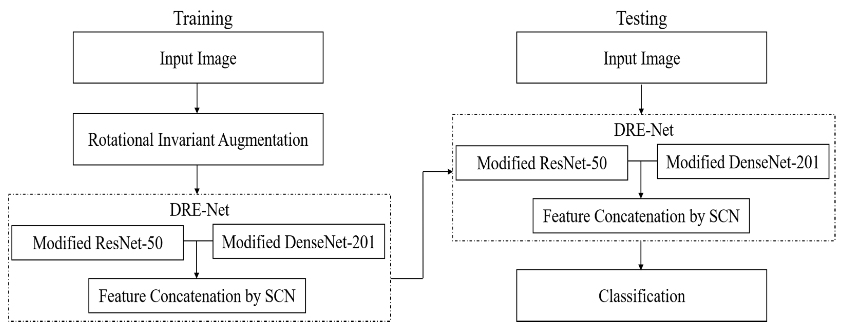
- To effectively identify shoulder implants, we propose a dense residual ensemble-network (DRE-Net) comprising two CNN models and a shallow concatenation network (SCN). Our network achieves a higher accuracy compared with state-of-the-art studies.
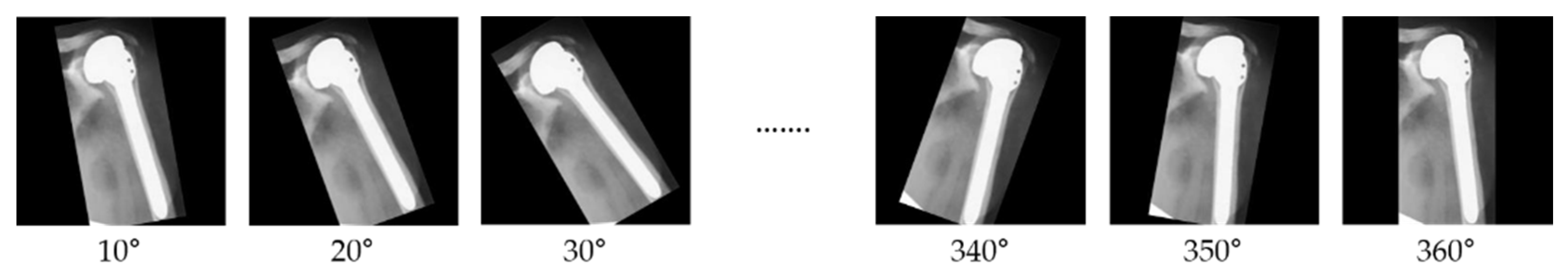
- We propose a rotational invariant augmentation (RIA) to tackle the overfitting problem.
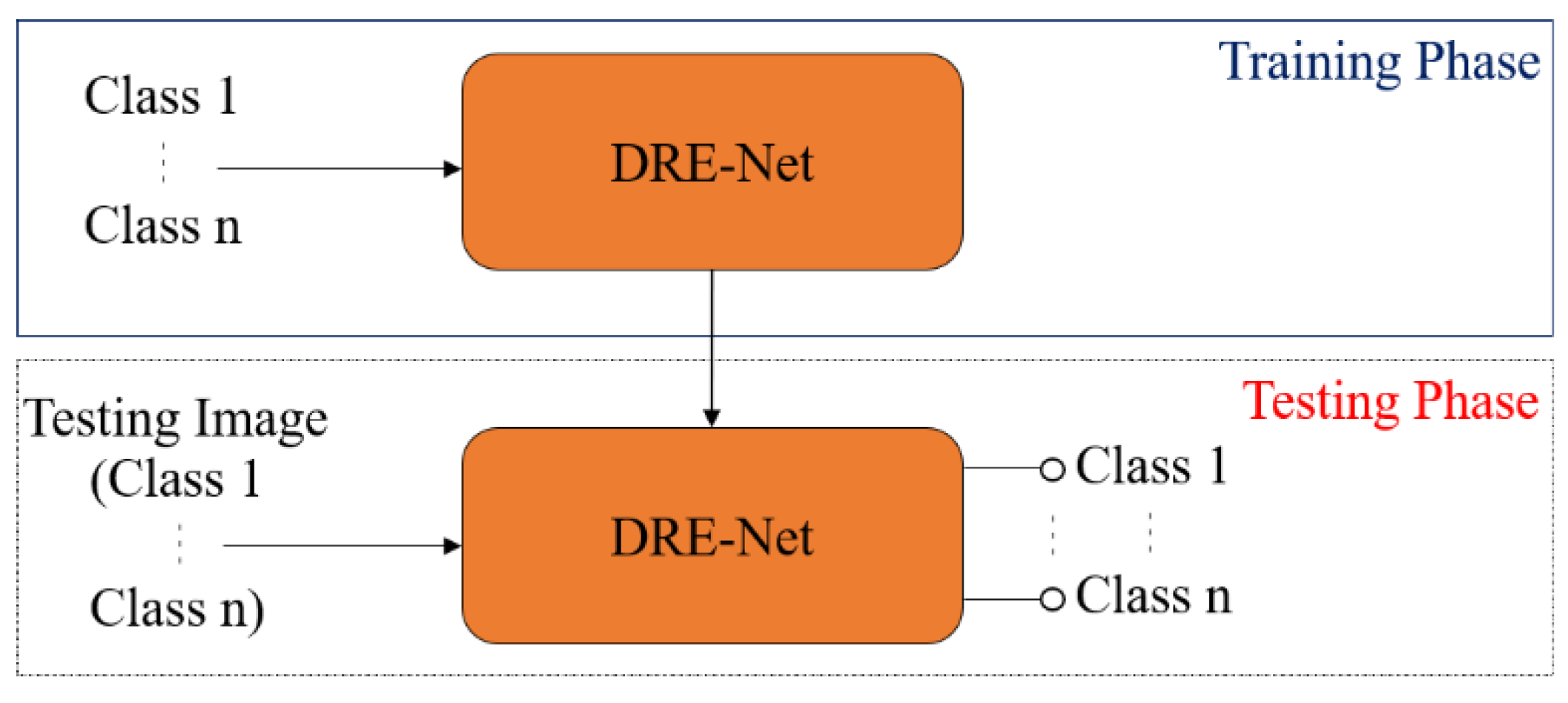
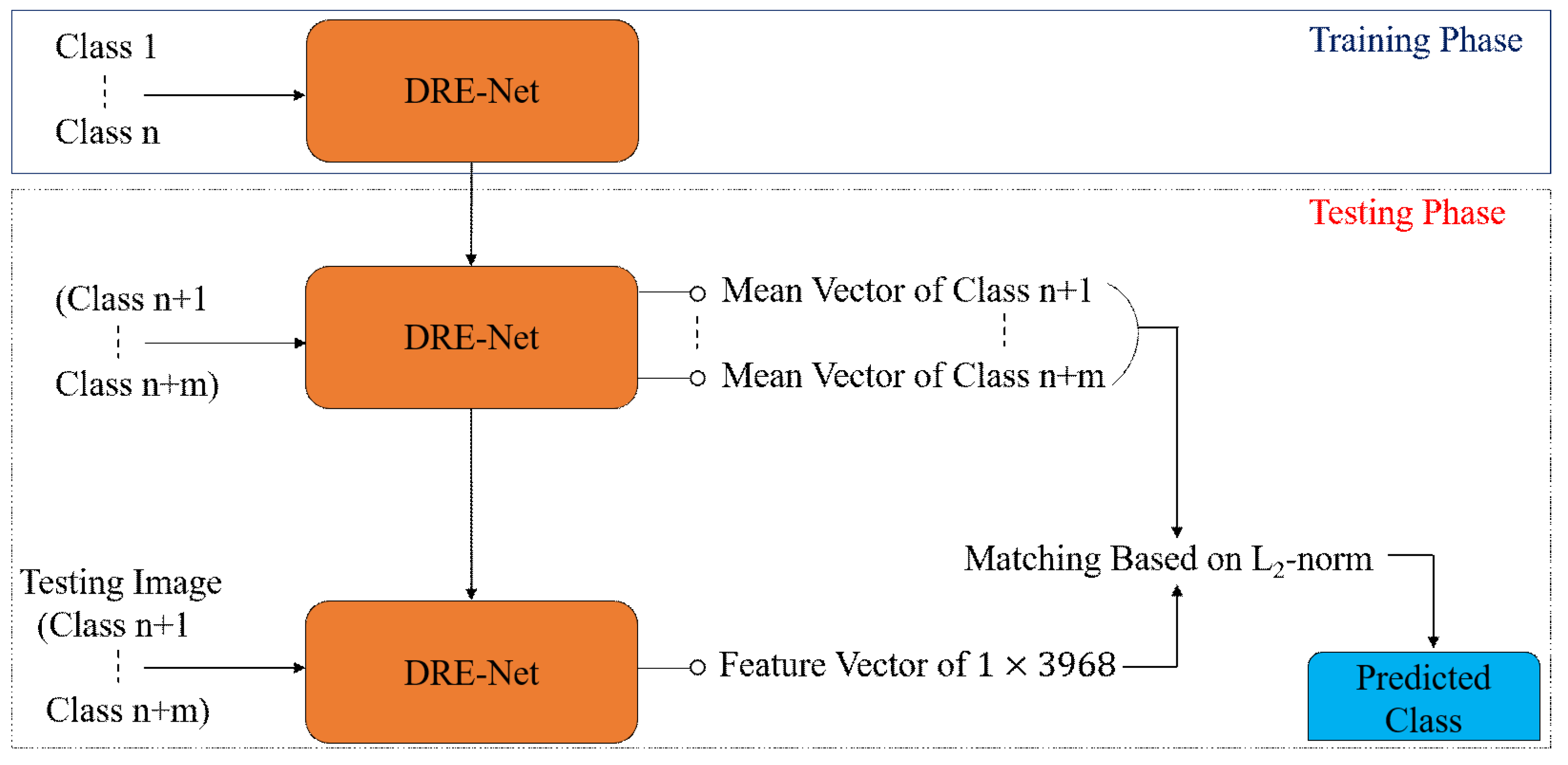
- To check the generalization capability of our network, the proposed DRE-Net is analyzed in different configuration modes of open and closed worlds.
- We analyzed the impact of end-to-end and sequential training of DRE-Net on the testing accuracy of shoulder implant images.
- Our model is publicly available [8] for a fair comparison by other researchers.
2. Related Works
3. Proposed Methods
3.1. Overview of Proposed Method
3.2. Rotational Invariant Augmentation (RIA)
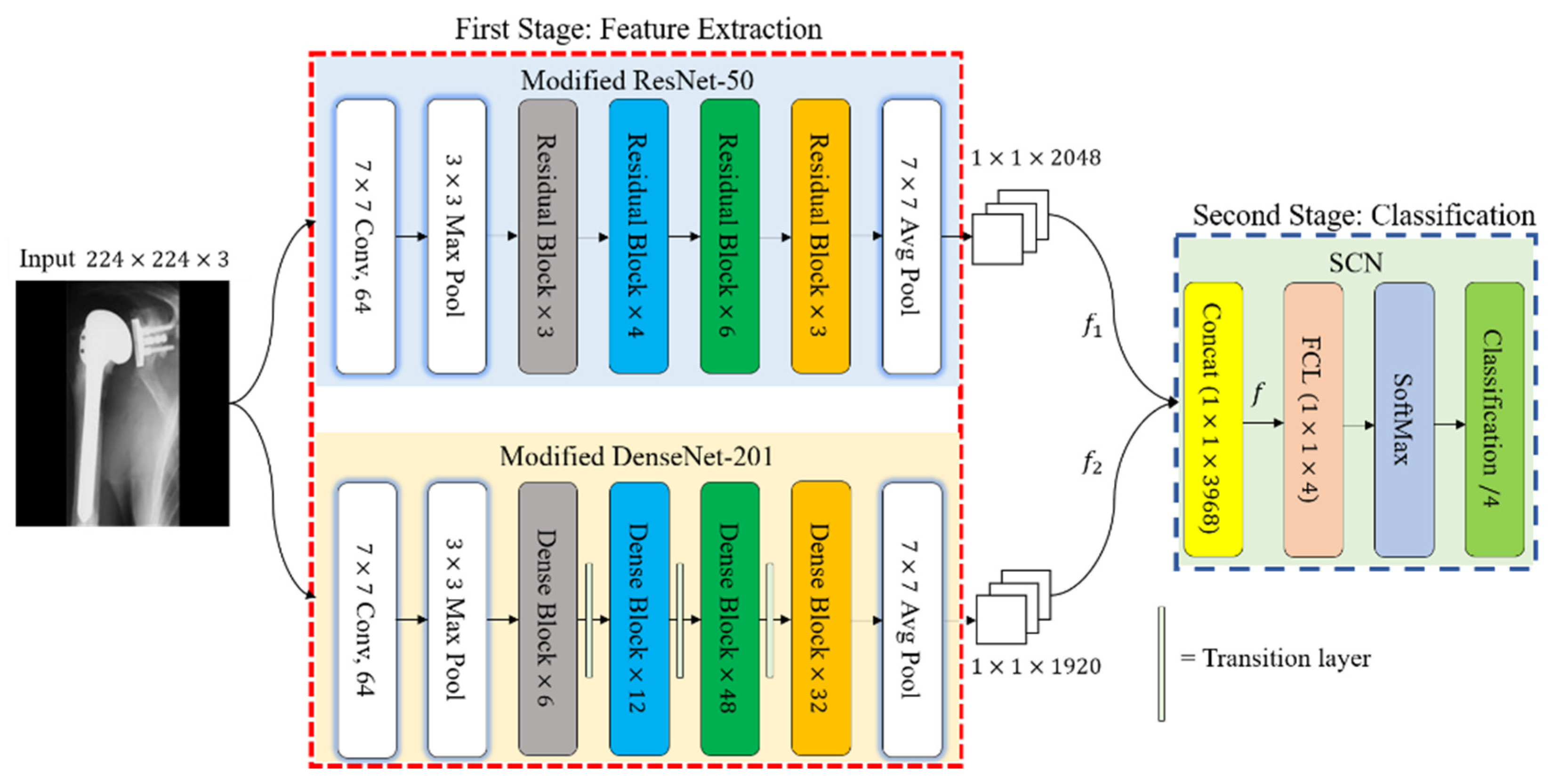
3.3. Classification of Shoulder Implants by DRE-Net
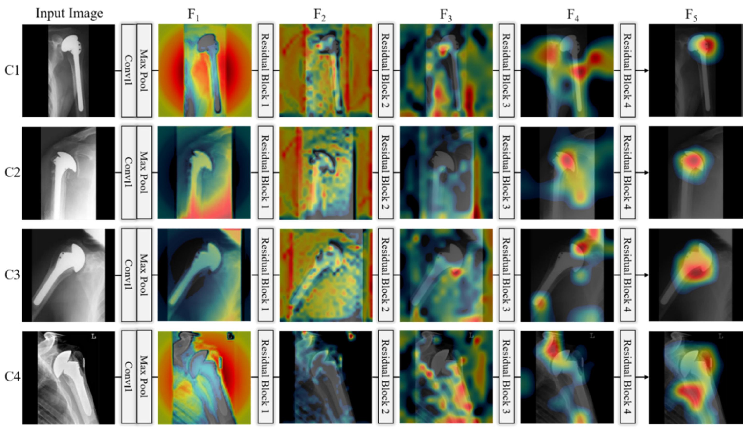
3.3.1. Feature Extraction Using Modified ResNet-50
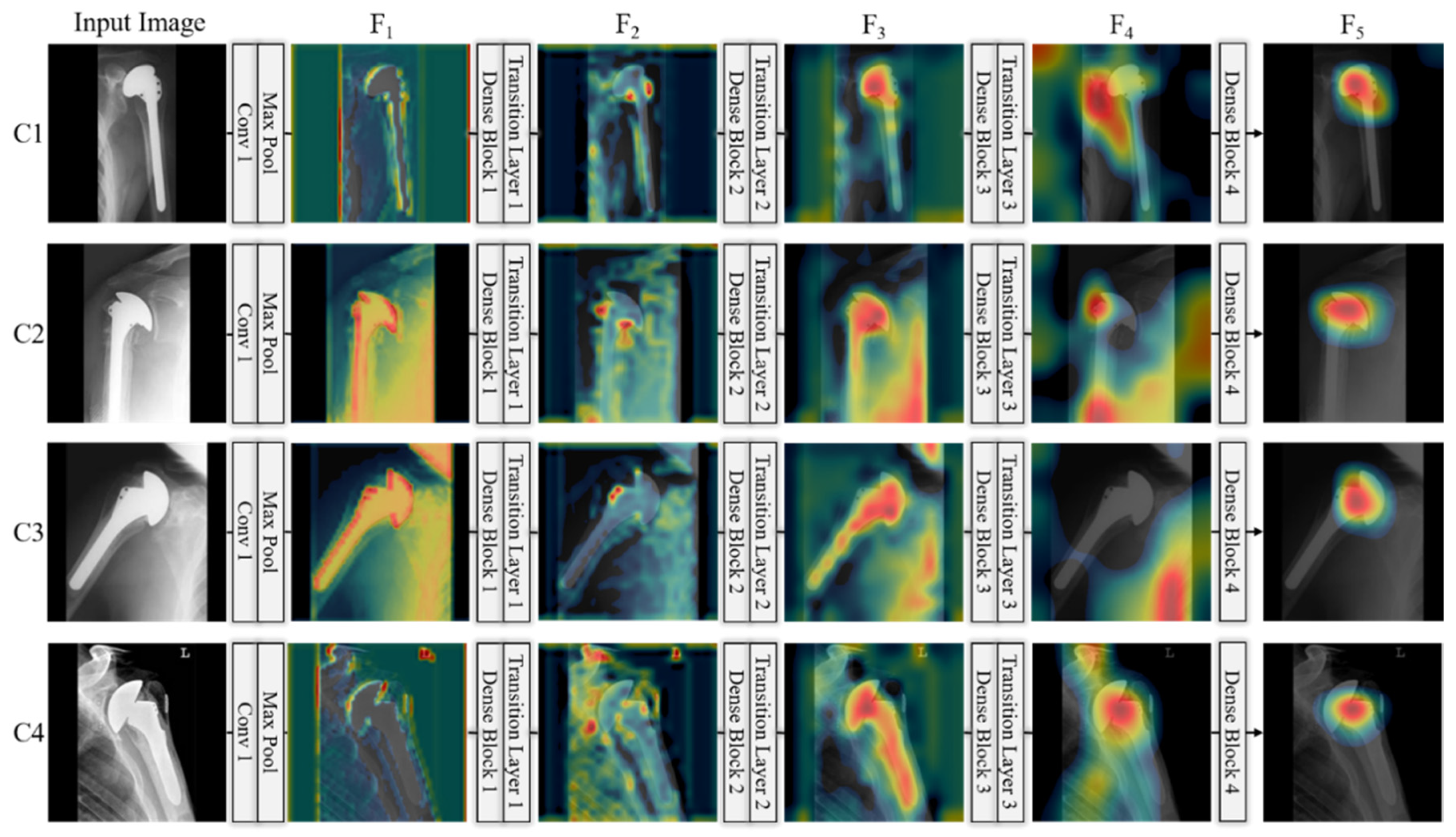
3.3.2. Feature Extraction Using Modified DenseNet-201
3.3.3. Feature Concatenation and Final Classification by SCN
3.4. Classification Configuration
4. Experimental Setups and Results
4.1. Dataset and Experimental Setups
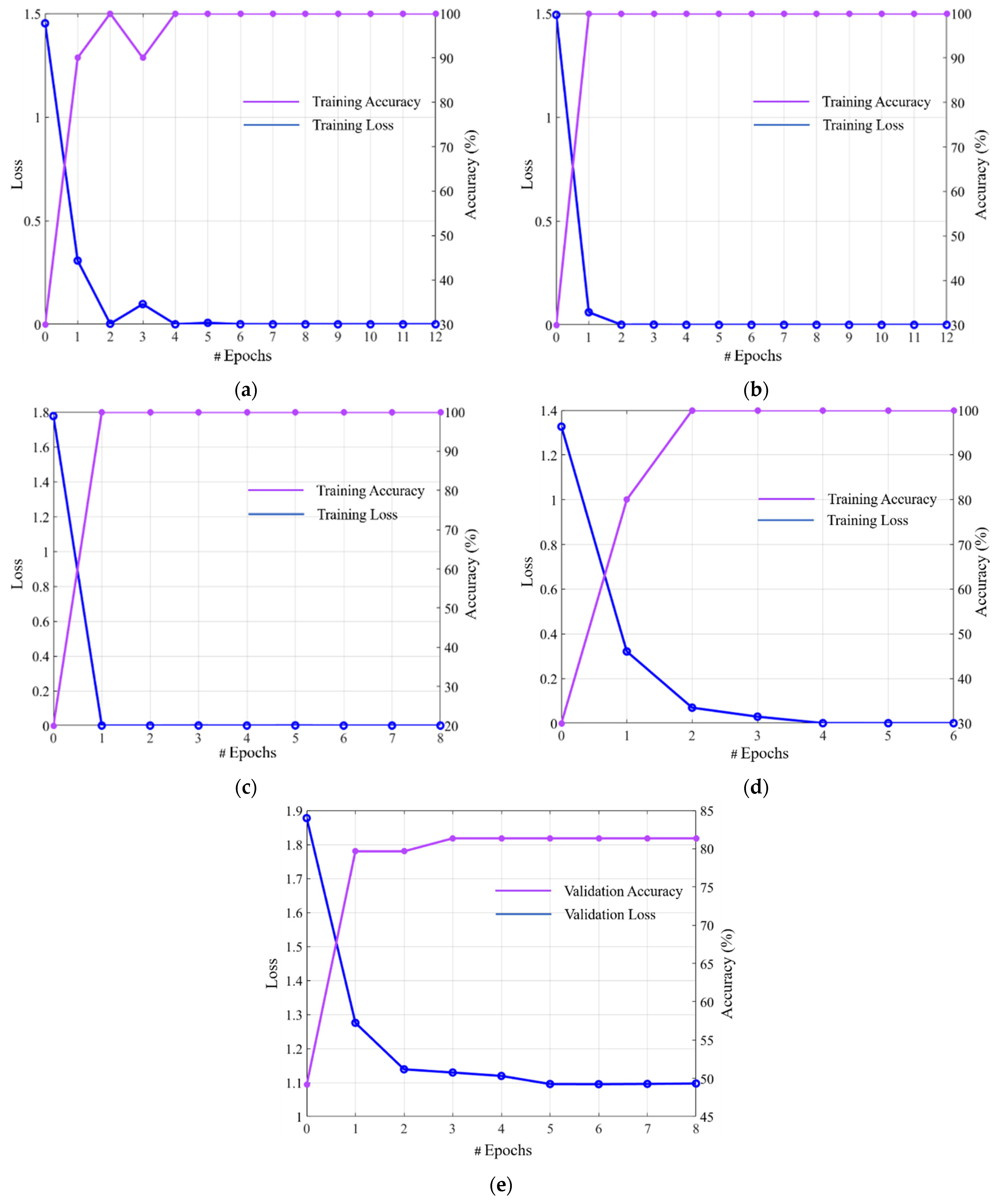
4.2. Training of CNN Model
4.3. Testing and Performance Analysis
4.3.1. Ablation Studies
4.3.2. Comparison of Proposed DRE-Net with the Subjective Evaluation
4.3.3. Comparisons of Proposed DRE-Net with the State-of-The-Art Methods
5. Discussions
6. Conclusions
Author Contributions
Funding
Institutional Review Board Statement
Informed Consent Statement
Data Availability Statement
Acknowledgments
Conflicts of Interest
References
- OrthoInfo, AAOS. Shoulder Joint Replacement. Available online: https://www.orthoinfo.org/en/treatment/shoulder-joint-replacement/ (accessed on 5 February 2021).
- Wicha, M.; Tomczyk-Warunek, A.; Jarecki, J.; Dubiel, A. Total Shoulder Arthroplasty, an Overview, Indications and Prosthetic Options. Wiad. Lek. 2020, 73, 1870–1873. [Google Scholar] [CrossRef]
- Burns, L.R.; Housman, M.G.; Booth, R.E.J.; Koenig, A. Implant Vendors and Hospitals: Competing Influences over Product Choice by Orthopedic Surgeons. Health Care Manag. Rev. 2009, 34, 2–18. [Google Scholar] [CrossRef]
- Mahomed, N.N.; Barrett, J.A.; Katz, J.N.; Phillips, C.B.; Losina, E.; Lew, R.A.; Guadagnoli, E.; Harris, W.H.; Poss, R.; Baron, J.A. Rates and Outcomes of Primary and Revision Total Hip Replacement in the United States Medicare Population. JBJS 2003, 85, 27–32. [Google Scholar] [CrossRef]
- Dy, C.J.; Bozic, K.J.; Padgett, D.E.; Pan, T.J.; Marx, R.G.; Lyman, S. Is Changing Hospitals for Revision Total Joint Arthroplasty Associated with More Complications? Clin. Orthop. Relat. Res. 2014, 472, 2006–2015. [Google Scholar] [CrossRef] [Green Version]
- Wilson, N.A.; Jehn, M.; York, S.; Davis, C.M. Revision Total Hip and Knee Arthroplasty Implant Identification: Implications for Use of Unique Device Identification 2012 AAHKS Member Survey Results. J. Arthroplast. 2014, 29, 251–255. [Google Scholar] [CrossRef]
- Branovacki, G. Ortho Atlas: Hip Arthroplasty U.S. Femoral Implants 1938–2008; Ortho Atlas Publishing: Chicago, IL, USA, 2008. [Google Scholar]
- CNN Models for Shoulder Implants Recognition with Algorithms. Available online: http://dm.dgu.edu/link.html (accessed on 6 February 2021).
- Bredow, J.; Wenk, B.; Westphal, R.; Wahl, F.; Budde, S.; Eysel, P.; Oppermann, J. Software-Based Matching of X-ray Images and 3D Models of Knee Prostheses. Technol. Health Care 2014, 22, 895–900. [Google Scholar] [CrossRef] [Green Version]
- Morais, P.; Queirós, S.; Moreira, A.H.J.; Ferreira, A.; Ferreira, E.; Duque, D.; Rodrigues, N.F.; Vilaça, J.L. Computer-Aided Recognition of Dental Implants in X-ray Images. In Proceedings of the SPIE 9414, Medical Imaging: Computer-Aided Diagnosis, Orlando, FL, USA, 20 March 2015; Volume 9414, p. 94142E. [Google Scholar]
- Stark, M.B.C.G. Automatic Detection and Segmentation of Shoulder Implants in X-ray Images. Master Thesis, San Francisco State University, San Francisco, CA, USA, 2018. [Google Scholar]
- Litjens, G.; Kooi, T.; Bejnordi, B.E.; Setio, A.A.A.; Ciompi, F.; Ghafoorian, M.; van der Laak, J.A.W.M.; van Ginneken, B.; Sánchez, C.I. A Survey on Deep Learning in Medical Image Analysis. Med. Image Anal. 2017, 42, 60–88. [Google Scholar] [CrossRef] [PubMed] [Green Version]
- Koteluk, O.; Wartecki, A.; Mazurek, S.; Kołodziejczak, I.; Mackiewicz, A. How Do Machines Learn? Artificial Intelligence as a New Era in Medicine. J. Pers. Med. 2021, 11, 32. [Google Scholar] [CrossRef]
- Owais, M.; Arsalan, M.; Choi, J.; Mahmood, T.; Park, K.R. Artificial Intelligence-Based Classification of Multiple Gastrointestinal Diseases Using Endoscopy Videos for Clinical Diagnosis. J. Clin. Med. 2019, 8, 986. [Google Scholar] [CrossRef] [Green Version]
- Owais, M.; Arsalan, M.; Choi, J.; Park, K.R. Effective Diagnosis and Treatment through Content-Based Medical Image Retrieval (CBMIR) by Using Artificial Intelligence. J. Clin. Med. 2019, 8, 462. [Google Scholar] [CrossRef] [Green Version]
- Mahmood, T.; Arsalan, M.; Owais, M.; Lee, M.B.; Park, K.R. Artificial Intelligence-Based Mitosis Detection in Breast Cancer Histopathology Images Using Faster R-CNN and Deep CNNs. J. Clin. Med. 2020, 9, 749. [Google Scholar] [CrossRef] [PubMed] [Green Version]
- Suh, Y.J.; Jung, J.; Cho, B.-J. Automated Breast Cancer Detection in Digital Mammograms of Various Densities via Deep Learning. J. Clin. Med. 2020, 10, 211. [Google Scholar] [CrossRef]
- Arsalan, M.; Baek, N.R.; Owais, M.; Mahmood, T.; Park, K.R. Deep Learning-Based Detection of Pigment Signs for Analysis and Diagnosis of Retinitis Pigmentosa. Sensors 2020, 20, 3454. [Google Scholar] [CrossRef]
- Arsalan, M.; Owais, M.; Mahmood, T.; Cho, S.W.; Park, K.R. Aiding the Diagnosis of Diabetic and Hypertensive Retinopathy Using Artificial Intelligence-Based Semantic Segmentation. J. Clin. Med. 2019, 8, 1446. [Google Scholar] [CrossRef] [Green Version]
- Arsalan, M.; Kim, D.S.; Owais, M.; Park, K.R. OR-Skip-Net: Outer Residual Skip Network for Skin Segmentation in Non-Ideal Situations. Expert Syst. Appl. 2020, 141, 112922. [Google Scholar] [CrossRef]
- Arsalan, M.; Owais, M.; Mahmood, T.; Choi, J.; Park, K.R. Artificial Intelligence-Based Diagnosis of Cardiac and Related Diseases. J. Clin. Med. 2020, 9, 871. [Google Scholar] [CrossRef] [Green Version]
- Arsalan, M.; Kim, D.S.; Lee, M.B.; Owais, M.; Park, K.R. FRED-Net: Fully Residual Encoder–Decoder Network for Accurate Iris Segmentation. Expert Syst. Appl. 2019, 122, 217–241. [Google Scholar] [CrossRef]
- Olczak, J.; Fahlberg, N.; Maki, A.; Razavian, A.S.; Jilert, A.; Stark, A.; Sköldenberg, O.; Gordon, M. Artificial Intelligence for Analyzing Orthopedic Trauma Radiographs: Deep Learning Algorithms-Are They on Par with Humans for Diagnosing Fractures? Acta Orthop. 2017, 88, 581–586. [Google Scholar] [CrossRef] [Green Version]
- Bini, S.A. Artificial Intelligence, Machine Learning, Deep Learning, and Cognitive Computing: What Do These Terms Mean and How Will They Impact Health Care? J. Arthroplast. 2018, 33, 2358–2361. [Google Scholar] [CrossRef]
- Tiulpin, A.; Thevenot, J.; Rahtu, E.; Lehenkari, P.; Saarakkala, S. Automatic Knee Osteoarthritis Diagnosis from Plain Radiographs: A Deep Learning-Based Approach. Sci. Rep. 2018, 8, 1727. [Google Scholar] [CrossRef]
- Chung, S.W.; Han, S.S.; Lee, J.W.; Oh, K.-S.; Kim, N.R.; Yoon, J.P.; Kim, J.Y.; Moon, S.H.; Kwon, J.; Lee, H.-J.; et al. Automated Detection and Classification of the Proximal Humerus Fracture by Using Deep Learning Algorithm. Acta Orthop. 2018, 89, 468–473. [Google Scholar] [CrossRef] [Green Version]
- Lindsey, R.; Daluiski, A.; Chopra, S.; Lachapelle, A.; Mozer, M.; Sicular, S.; Hanel, D.; Gardner, M.; Gupta, A.; Hotchkiss, R.; et al. Deep Neural Network Improves Fracture Detection by Clinicians. Proc. Natl. Acad. Sci. USA 2018, 115, 11591–11596. [Google Scholar] [CrossRef] [PubMed] [Green Version]
- Kitamura, G.; Chung, C.Y.; Moore, B.E. Ankle Fracture Detection Utilizing a Convolutional Neural Network Ensemble Implemented with a Small Sample, De Novo Training, and Multiview Incorporation. J. Digit. Imaging 2019, 32, 672–677. [Google Scholar] [CrossRef] [Green Version]
- Rayan, J.C.; Reddy, N.; Kan, J.H.; Zhang, W.; Annapragada, A. Binomial Classification of Pediatric Elbow Fractures Using a Deep Learning Multiview Approach Emulating Radiologist Decision Making. Radiol. Artif. Intell. 2019, 1, e180015. [Google Scholar] [CrossRef]
- Borjali, A.; Chen, A.F.; Muratoglu, O.K.; Morid, M.A.; Varadarajan, K.M. Detecting Mechanical Loosening of Total Hip Replacement Implant from Plain Radiograph Using Deep Convolutional Neural Network. arXiv 2019, arXiv:1912.00943v1. Available online: https://arxiv.org/abs/1912.00943 (accessed on 7 February 2021).
- Krogue, J.D.; Cheng, K.V.; Hwang, K.M.; Toogood, P.; Meinberg, E.G.; Geiger, E.J.; Zaid, M.; McGill, K.C.; Patel, R.; Sohn, J.H.; et al. Automatic Hip Fracture Identification and Functional Subclassification with Deep Learning. Radiol. Artif. Intell. 2020, 2, e190023. [Google Scholar] [CrossRef] [Green Version]
- Yi, P.H.; Wei, J.; Kim, T.K.; Sair, H.I.; Hui, F.K.; Hager, G.D.; Fritz, J.; Oni, J.K. Automated Detection & Classification of Knee Arthroplasty Using Deep Learning. Knee 2020, 27, 535–542. [Google Scholar] [CrossRef]
- Karnuta, J.M.; Luu, B.C.; Roth, A.L.; Haeberle, H.S.; Chen, A.F.; Iorio, R.; Schaffer, J.L.; Mont, M.A.; Patterson, B.M.; Krebs, V.E.; et al. Artificial Intelligence to Identify Arthroplasty Implants from Radiographs of the Knee. J. Arthroplast. 2021, 36, 935–940. [Google Scholar] [CrossRef]
- Sukegawa, S.; Yoshii, K.; Hara, T.; Yamashita, K.; Nakano, K.; Yamamoto, N.; Nagatsuka, H.; Furuki, Y. Deep Neural Networks for Dental Implant System Classification. Biomolecules 2020, 10, 984. [Google Scholar] [CrossRef]
- Kim, J.-E.; Nam, N.-E.; Shim, J.-S.; Jung, Y.-H.; Cho, B.-H.; Hwang, J.J. Transfer Learning via Deep Neural Networks for Implant Fixture System Classification Using Periapical Radiographs. J. Clin. Med. 2020, 9, 1117. [Google Scholar] [CrossRef] [Green Version]
- Iandola, F.N.; Han, S.; Moskewicz, M.W.; Ashraf, K.; Dally, W.J.; Keutzer, K. SqueezeNet: AlexNet-Level Accuracy with 50× Fewer Parameters and <0.5 MB Model Size. arXiv 2016, arXiv:1602.07360v4. Available online: https://arxiv.org/abs/1602.07360v4?source=post_page (accessed on 9 February 2021).
- Szegedy, C.; Liu, W.; Jia, Y.; Sermanet, P.; Reed, S.; Anguelov, D.; Erhan, D.; Vanhoucke, V.; Rabinovich, A. Going Deeper with Convolutions. In Proceedings of the IEEE Conference on Computer Vision and Pattern Recognition, Boston, MA, USA, 7–12 June 2015; pp. 1–9. [Google Scholar] [CrossRef] [Green Version]
- He, K.; Zhang, X.; Ren, S.; Sun, J. Deep Residual Learning for Image Recognition. In Proceedings of the IEEE Conference on Computer Vision and Pattern Recognition, Las Vegas, NV, USA, 27–30 June 2016; pp. 770–778. [Google Scholar] [CrossRef] [Green Version]
- Sandler, M.; Howard, A.; Zhu, M.; Zhmoginov, A.; Chen, L.-C. MobileNetV2: Inverted Residuals and Linear Bottlenecks. In Proceedings of the IEEE Conference on Computer Vision and Pattern Recognition, Salt Lake City, UT, USA, 18–23 June 2018; pp. 4510–4520. [Google Scholar] [CrossRef] [Green Version]
- Borjali, A.; Chen, A.F.; Muratoglu, O.K.; Morid, M.A.; Varadarajan, K.M. Detecting Total Hip Replacement Prosthesis Design on Plain Radiographs Using Deep Convolutional Neural Network. J. Orthop. Res. 2020, 38, 1465–1471. [Google Scholar] [CrossRef] [Green Version]
- Huang, G.; Liu, Z.; van der Maaten, L.; Weinberger, K.Q. Densely Connected Convolutional Networks. In Proceedings of the IEEE Conference on Computer Vision and Pattern Recognition, Honolulu, HI, USA, 21–26 July 2017; pp. 4700–4708. [Google Scholar] [CrossRef] [Green Version]
- Deng, J.; Dong, W.; Socher, R.; Li, L.-J.; Li, K.; Fei-Fei, L. ImageNet: A Large-scale Hierarchical Image Database. In Proceedings of the IEEE Conference on Computer Vision and Pattern Recognition, Miami, FL, USA, 20–25 June 2009; pp. 248–255. [Google Scholar]
- Pranata, Y.D.; Wang, K.-C.; Wang, J.-C.; Idram, I.; Lai, J.-Y.; Liu, J.-W.; Hsieh, I.-H. Deep Learning and SURF for Automated Classification and Detection of Calcaneus Fractures in CT Images. Comput. Meth. Programs Biomed. 2019, 171, 27–37. [Google Scholar] [CrossRef]
- Tanzi, L.; Vezzetti, E.; Moreno, R.; Aprato, A.; Audisio, A.; Massè, A. Hierarchical Fracture Classification of Proximal Femur X-ray Images Using a Multistage Deep Learning Approach. Eur. J. Radiol. 2020, 133, 109373. [Google Scholar] [CrossRef]
- Urban, G.; Porhemmat, S.; Stark, M.; Feeley, B.; Okada, K.; Baldi, P. Classifying Shoulder Implants in X-ray Images Using Deep Learning. Comp. Struct. Biotechnol. J. 2020, 18, 967–972. [Google Scholar] [CrossRef] [PubMed]
- Yi, P.H.; Kim, T.K.; Wei, J.; Li, X.; Hager, G.D.; Sair, H.I.; Fritz, J. Automated Detection and Classification of Shoulder Arthroplasty Models Using Deep Learning. Skelet. Radiol. 2020, 49, 1623–1632. [Google Scholar] [CrossRef] [PubMed]
- Shorten, C.; Khoshgoftaar, T.M. A Survey on Image Data Augmentation for Deep Learning. J. Big Data 2019, 6, 60. [Google Scholar] [CrossRef]
- Polikar, R. Ensemble Based Systems in Decision Making. IEEE Circuits Syst. Mag. 2006, 6, 21–45. [Google Scholar] [CrossRef]
- Rokach, L. Ensemble-Based Classifiers. Artif. Intell. Rev. 2010, 33, 1–39. [Google Scholar] [CrossRef]
- Krizhevsky, A.; Sutskever, I.; Hinton, G.E. ImageNet Classification with Deep Convolutional Neural Networks. In Proceedings of the 25th International Conference on Neural Information Processing Systems, Lake Tahoe, NV, USA, 3–8 December 2012; pp. 1097–1105. [Google Scholar] [CrossRef]
- ImageNet. Available online: http://www.image-net.org/ (accessed on 7 February 2021).
- Glorot, X.; Bordes, A.; Bengio, Y. Deep Sparse Rectifier Neural Networks. In Proceedings of the 14th International Conference on Artificial Intelligence and Statistics, Fort Lauderdale, FL, USA, 11–13 April 2011; pp. 315–323. [Google Scholar]
- Ioffe, S.; Szegedy, C. Batch Normalization: Accelerating Deep Network Training by Reducing Internal Covariate Shift. In Proceedings of the International Conference on Machine Learning, Lille, France, 7–9 July 2015; pp. 448–456. [Google Scholar]
- Zheng, L.; Zhao, Y.; Wang, S.; Wang, J.; Tian, Q. Good Practice in CNN Feature Transfer. arXiv 2016, arXiv:1604.00133v1. Available online: https://arxiv.org/abs/1604.00133 (accessed on 9 February 2021).
- Kawahara, J.; Hamarneh, G. Multi-Resolution-Tract CNN with Hybrid Pretrained and Skin-Lesion Trained Layers. In Proceedings of the International Workshop on Machine Learning in Medical Imaging, Athens, Greece, 17 October 2016; pp. 164–171. [Google Scholar]
- Goodfellow, I.; Bengio, Y.; Courville, A. Deep Learning; MIT Press: Cambridge, MA, USA, 2016; Volume 1. [Google Scholar]
- Heesch, D. A Survey of Browsing Models for Content Based Image Retrieval. Multimed. Tools Appl. 2008, 40, 261–284. [Google Scholar] [CrossRef]
- Buda, M.; Maki, A.; Mazurowski, M.A. A Systematic Study of the Class Imbalance Problem in Convolutional Neural Networks. Neural Netw. 2018, 106, 249–259. [Google Scholar] [CrossRef] [Green Version]
- Intel® Core™ i7-3770K Processor. Available online: https://ark.intel.com/content/www/us/en/ark/products/65523/intel-core-i7-3770k-processor-8m-cache-up-to-3-90-ghz.html (accessed on 1 December 2020).
- GeForce GTX 1070. Available online: https://www.geforce.com/hardware/desktop-gpus/geforce-gtx-1070/specifications (accessed on 1 December 2020).
- Deep Learning Toolbox. Available online: https://www.mathworks.com/products/deep-learning.html (accessed on 1 December 2020).
- Heaton, J. Artificial Intelligence for Humans, Volume 3—Deep Learning and Neural Networks; Heaton Research, Inc.: St. Louis, MO, USA, 2013; ISBN 978-1-5057-1434-0. [Google Scholar]
- Ruder, S. An Overview of Gradient Descent Optimization Algorithms. arXiv 2017, arXiv:1609.04747v2. Available online: https://arxiv.org/abs/1609.04747 (accessed on 9 February 2021).
- Options for Training Deep Learning Neural Network. Available online: https://www.mathworks.com/help/deeplearning/ref/trainingoptions.html (accessed on 13 February 2021).
- Hossin, M. A Review on Evaluation Metrics for Data Classification Evaluations. Int. J. Data Min. Knowl. Manag. Process 2015, 5, 1–11. [Google Scholar] [CrossRef]
- Abdi, H.; Williams, L.J. Principal Component Analysis. WIREs Comput. Stat. 2010, 2, 433–459. [Google Scholar] [CrossRef]
- Cover, T.; Hart, P. Nearest Neighbor Pattern Classification. IEEE Trans. Inf. Theory 1967, 13, 21–27. [Google Scholar] [CrossRef]
- Kuncheva, L.I.; Whitaker, C.J. Measures of Diversity in Classifier Ensembles and Their Relationship with the Ensemble Accuracy. Mach. Learn. 2003, 51, 181–207. [Google Scholar] [CrossRef]
- Simonyan, K.; Zisserman, A. Very Deep Convolutional Networks for Large-Scale Image Recognition. arXiv 2015, arXiv:1409.1556v6. Available online: https://arxiv.org/abs/1409.1556 (accessed on 11 February 2021).
- Zoph, B.; Vasudevan, V.; Shlens, J.; Le, Q.V. Learning Transferable Architectures for Scalable Image Recognition. In Proceedings of the IEEE Conference on Computer Vision and Pattern Recognition, Salt Lake City, UT, USA, 18–23 June 2018; pp. 8697–8710. [Google Scholar] [CrossRef] [Green Version]
- Livingston, E.H. Who Was Student and Why Do We Care so Much about His T-Test? J. Surg. Res. 2004, 118, 58–65. [Google Scholar] [CrossRef]
- Zhou, B.; Khosla, A.; Lapedriza, A.; Oliva, A.; Torralba, A. Learning Deep Features for Discriminative Localization. In Proceedings of the IEEE Conference on Computer Vision and Pattern Recognition, Las Vegas, NV, USA, 27–30 June 2016; pp. 2921–2929. [Google Scholar]
- Krawczyk, B. Learning from Imbalanced Data: Open Challenges and Future Directions. Prog. Artif. Intell. 2016, 5, 221–232. [Google Scholar] [CrossRef] [Green Version]


| Category | Type | Methods | # Classes | Results | Strength | Weakness |
|---|---|---|---|---|---|---|
| Handcrafted feature-based | Knee | Template matching [9] | 1 | 70% to 90% accuracies | - Uses a simple image processing technique including Sobel operator, binarization, and template matching - Computationally efficient | Requires 3D CAD models for template generation of implants |
| Dental | Active contours + K-nearest neighborhood (K-NN) [10] | 11 | 91% of the known implants are recognized | - Optimal initial location of the contour can be selected by their method - Uses simple machine learning algorithm for classification | - K-NN classifier is time-consuming for large numbers of features - Because of the large number of dental implant models, their approach returns a set of possible candidate results for identifying new implants and needs a user interaction to verify the candidate result | |
| Shoulder | Hough transform + histogram equalization + mean shift filter [11] | 4 | 77% precision, and 64% F-measure | - Uses conventional image processing schemes involving bilateral filter, mean shift filter, and a median blur filter - Develops a pre-processing tool for training a classifier | Segmentation performance is dependent on the growing approach of seed region | |
| Deep feature-based | Knee | Pre-trained CNN [32] | 2 | 100% sensitivity, and 100% specificity | - High classification performance - Precisely determines the presence of total knee arthroplasty (TKA) - Accurately classifies the TKA and unicompartmental knee arthroplasty (UKA) | Classification is performed in a binary fashion (the presence of implant) |
| Pre-trained CNN [33] | 9 | 99% accuracy, 95% sensitivity, and 99% specificity | High classification performance | Pre-processing is needed and computationally expensive | ||
| Dental | Pre-trained CNN [34] | 11 | 93.5% accuracy, 91.6% F-measures | High average classification accuracy with a small dataset of panoramas | VGG network can be replaced with the state-of-the-art networks | |
| Pre-trained CNN [35] | 4 | 96% to 97% accuracies | High classification performance and computationally efficient | Their method is unable to detect several implants simultaneously | ||
| Hip | Pre-trained CNN [40] | 3 | 100% accuracy | High classification performance | - Requires high processing power for extensive training - Uses only one post-surgery anteroposterior (AP) X-ray per patient | |
| Shoulder | Pre-trained CNN [46] | 2 | 95% sensitivity, and 90% specificity to classify TSA and RTSA | - High accuracy to detect the existence of shoulder arthroplasty - High sensitivity to classify TSA and RTSA | Classification is performed in a binary fashion (the presence of implant) | |
| Pre-trained CNN [45] | 4 | 80.4% accuracy, 80% precision, 75% recall, and 76% F1-score | - First deep learning based-approach to classify the manufacturers of shoulder implants - Higher classification accuracy than non-deep learning-based methods | - Accuracies are needed to be enhanced - Performance was measured only by closed-world configuration | ||
| DRE-Net (Proposed) | 4 | 85.92% accuracy, 84.69% F1-score, 85.33% precision, and 84.11% recall | - High classification accuracy - Applicable to real-world problems by considering both closed-world and open-world configurations | Requires more training time |
| Layers Name | Output Feature Map Size | Kernel Size | Number of Iterations |
|---|---|---|---|
| Image Input | - | - | |
| Conv 1 | 1 | ||
| Max Pooling | 1 | ||
| Conv 2_x | 3 | ||
| Conv 3_x | 4 | ||
| Conv 4_x | 6 | ||
| Conv 5_x | 3 | ||
| Average Pooling | 1 |
| Layer Name | Output Feature Map Size | Kernel Size | Number of Iterations |
|---|---|---|---|
| Image Input | - | - | |
| Conv 1 | 1 | ||
| Max Pooling | 1 | ||
| DenseBlock_1 | 6 | ||
| Transition Layer | 1 | ||
| DenseBlock_2 | 12 | ||
| Transition Layer | 1 | ||
| DenseBlock_3 | 48 | ||
| Transition Layer | 1 | ||
| DenseBlock_4 | 32 | ||
| Average Pooling | 1 |
| Layers Name | Output Feature Map Size | Kernel Size | Number of Iterations |
|---|---|---|---|
| Concat | - | 1 | |
| Fully Connected | - | 1 | |
| SoftMax | - | 1 | |
| Classification | - | 1 |
| Validation | Training | Testing | Total | ||||
|---|---|---|---|---|---|---|---|
| Original | Augmented | C1 | C2 | C3 | C4 | ||
| 1st fold | 538 | 19,368 | 8 | 29 | 7 | 15 | 19,965 |
| 2nd fold | 536 | 19,296 | 9 | 30 | 7 | 15 | 19,893 |
| 3rd fold | 538 | 19,368 | 8 | 29 | 7 | 15 | 19,965 |
| 4th fold | 537 | 19,332 | 8 | 30 | 7 | 15 | 19,929 |
| 5th fold | 536 | 19,296 | 9 | 29 | 8 | 15 | 19,893 |
| 6th fold | 539 | 19,404 | 8 | 29 | 7 | 14 | 20,001 |
| 7th fold | 537 | 19,332 | 8 | 30 | 7 | 15 | 19,929 |
| 8th fold | 538 | 19,368 | 8 | 29 | 7 | 15 | 19,965 |
| 9th fold | 536 | 19,296 | 9 | 30 | 7 | 15 | 19,893 |
| 10th fold | 538 | 19,368 | 8 | 29 | 7 | 15 | 19,965 |
| Methods | Number of Epochs | Mini-Batch Size | Learning Rate | Momentum Term | L2-Regularization | Learning Rate Drop Factor | |
|---|---|---|---|---|---|---|---|
| Sequential training | Modified DenseNet-201 | 13 | 10 | 0.001 | 0.9 | 0.0001 | 0.1 |
| Modified ResNet-50 | 13 | 10 | 0.001 | 0.9 | 0.0001 | 0.1 | |
| SCN | 9 | 10 | 0.001 | 0.9 | 0.0001 | 0.1 | |
| End-to-end training | DRE-Net | 7 | 10 | 0.001 | 0.9 | 0.0001 | 0.1 |
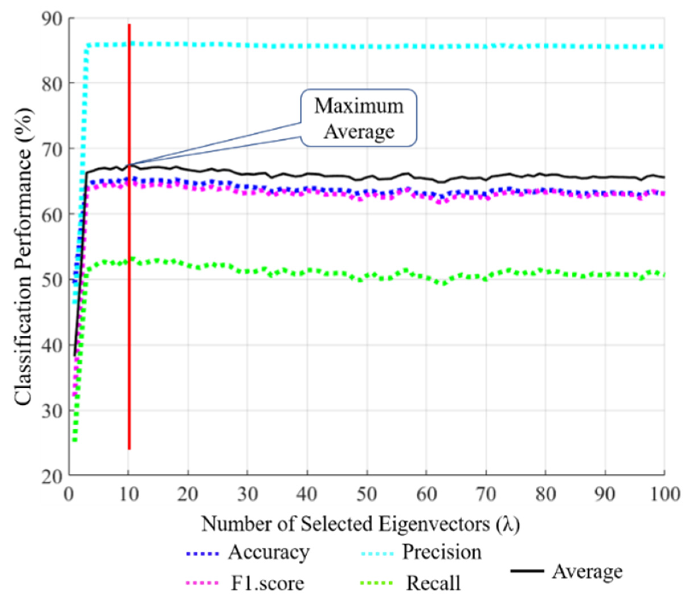
| Fold | Performance without a PCA (our SCN) | Performance with PCA (λ = 10) + K-NN | ||||||
|---|---|---|---|---|---|---|---|---|
| Accuracy | F1-Score | Recall | Precision | Accuracy | F1-Score | Recall | Precision | |
| 10-Fold Average | 85.92 | 84.69 | 84.11 | 85.33 | 57.94 | 48.04 | 40.60 | 60.17 |
| Methods | Accuracy | F1-Score | Precision | Recall |
|---|---|---|---|---|
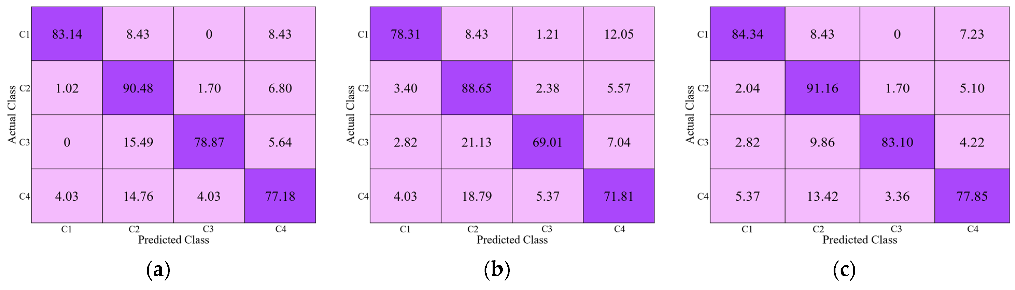
| ResNet-50 [38] | 66.70 | 62.02 | 64.67 | 59.83 |
| DenseNet-201 [41] | 55.76 | 47.55 | 49.73 | 45.73 |
| ResNet-50 + RIA | 80.57 | 78.02 | 79.21 | 76.95 |
| DenseNet-201 + RIA | 84.75 | 83.76 | 85.21 | 82.42 |
| DRE-Net (end-to-end) | 81.55 | 79.12 | 80.77 | 77.66 |
| DRE-Net (sequential) | 85.92 | 84.69 | 85.33 | 84.11 |
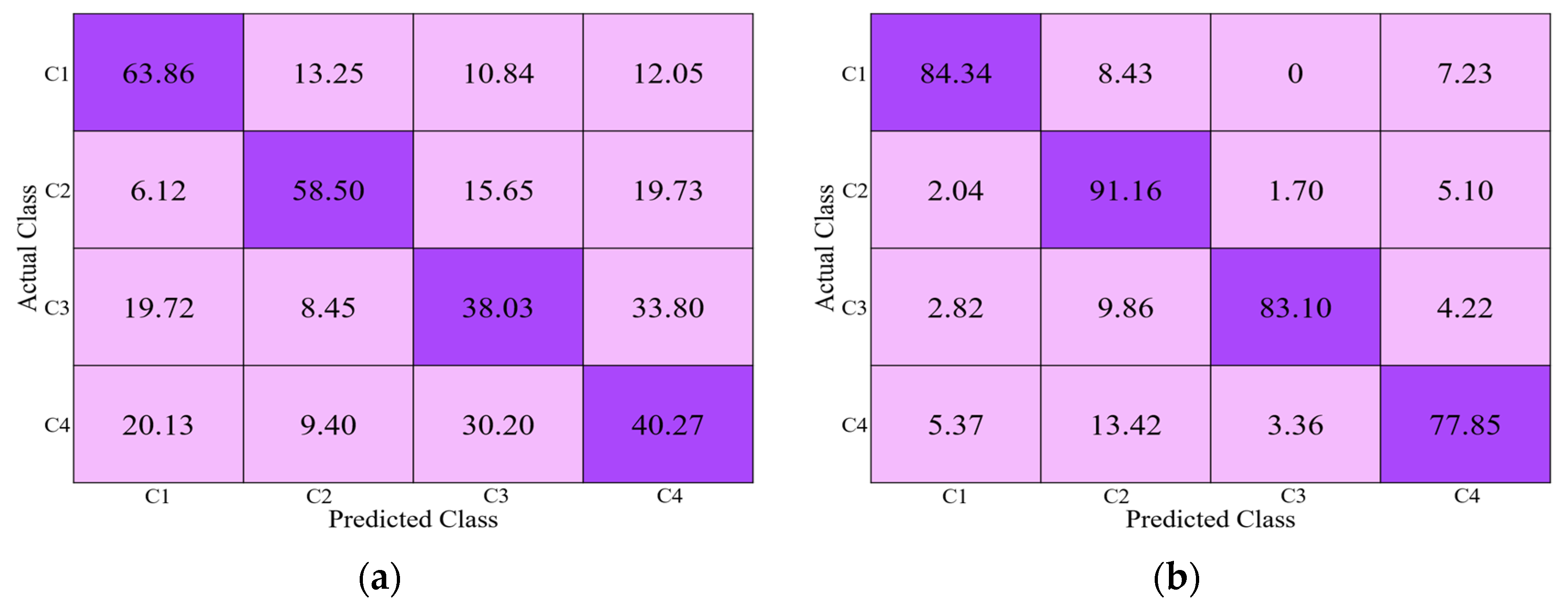
| Demographic Details | Subjective Performance (%) | ||||||
|---|---|---|---|---|---|---|---|
| Participant Index | Age | Nationality | Sex | Accuracy | F1-Score | Precision | Recall |
| 1 | 28 | Pakistan | Male | 57.63 | 53.40 | 53.51 | 53.29 |
| 2 | 28 | Pakistan | Male | 55.74 | 48.86 | 49.23 | 48.49 |
| 3 | 23 | South Korea | Male | 50.85 | 55.35 | 55.51 | 55.19 |
| 4 | 32 | Pakistan | Male | 48.33 | 48.43 | 46.90 | 50.06 |
| 5 | 27 | South Korea | Male | 50.82 | 45.58 | 45.51 | 45.66 |
| 6 | 29 | South Korea | Male | 55.17 | 45.67 | 45.13 | 46.23 |
| 7 | 42 | Iran | Female | 58.33 | 54.87 | 52.92 | 56.96 |
| 8 | 27 | South Korea | Female | 45.76 | 42.83 | 41.84 | 43.88 |
| 9 | 32 | Pakistan | Male | 52.46 | 46.77 | 46.63 | 46.90 |
| 10 | 28 | South Korea | Male | 47.46 | 53.68 | 51.47 | 56.09 |
| Methods | Accuracy | F1-Score | Precision | Recall |
|---|---|---|---|---|
| Subjective Method | 52.25 | 49.54 | 48.86 | 50.28 |
| DRE-Net (sequential) | 85.92 | 84.69 | 85.33 | 84.11 |
| Methods | Accuracy | F1-Score | Precision | Recall |
|---|---|---|---|---|
| VGG-16 [45,69] | 58.70 | 45 | 54 | 45 |
| VGG-19 [45,69] | 63.60 | 54 | 61 | 53 |
| ResNet-18 [38,46] | 66.13 | 60.86 | 64.25 | 58.13 |
| ResNet-50 [38] | 66.70 | 62.02 | 64.67 | 59.83 |
| NASNet [45,70] | 64.50 | 54 | 62 | 52 |
| DenseNet-201 [41] | 55.76 | 47.55 | 49.73 | 45.73 |
| Proposed | 58.10 | 50.82 | 51.78 | 49.96 |
| Methods | Accuracy | F1-Score | Precision | Recall |
|---|---|---|---|---|
| VGG-16 [45,69] | 74 | 69 | 72 | 68 |
| VGG-19 [45,69] | 76.20 | 70 | 75 | 69 |
| ResNet-18 [38,46] | 70.82 | 65.93 | 68.02 | 64.38 |
| ResNet-50 [38] | 80.56 | 77.66 | 79.49 | 76.02 |
| NASNet [45,70] | 80.40 | 76 | 80 | 75 |
| DenseNet-201 [41] | 80.57 | 77.60 | 79.05 | 76.32 |
| Proposed | 77.05 | 74.80 | 76.93 | 73.07 |
| Methods | Accuracy | F1-Score | Precision | Recall |
|---|---|---|---|---|
| VGG-16 [45,69] | 68.85 | 66.90 | 66.82 | 67.22 |
| VGG-19 [45,69] | 66.54 | 63.54 | 63.81 | 63.35 |
| ResNet-18 [38,46] | 77.41 | 74.67 | 76.60 | 73.05 |
| ResNet-50 [38] | 80.57 | 78.02 | 79.21 | 76.95 |
| NASNet [45,70] | 79.23 | 76.28 | 77.25 | 75.44 |
| DenseNet-201 [41] | 84.75 | 83.76 | 85.21 | 82.42 |
| Proposed | 85.92 | 84.69 | 85.33 | 84.11 |
| Comparisons | p-Value | Confidence Level | |
|---|---|---|---|
| Proposed | Second-best | 0.03 | 97% |
| Proposed | Third-best | 7.84 × 10⁻⁹ | 99% |
| Validation | Training | Testing | ||||
|---|---|---|---|---|---|---|
| Classes | Original | Augmented | Classes | Original | Total | |
| 1st fold-A | Cofield, Depuy | 377 | 13,572 | Tornier, Zimmer | 220 | 14,169 |
| 1st fold-B | Tornier, Zimmer | 220 | 7920 | Cofield, Depuy | 377 | 8517 |
| 2nd fold-A | Tornier, Cofield | 154 | 5544 | Zimmer, Depuy | 443 | 3585 |
| 2nd fold-B | Zimmer, Depuy | 443 | 15,948 | Tornier, Cofield | 154 | 16,545 |
Publisher’s Note: MDPI stays neutral with regard to jurisdictional claims in published maps and institutional affiliations. |
© 2021 by the authors. Licensee MDPI, Basel, Switzerland. This article is an open access article distributed under the terms and conditions of the Creative Commons Attribution (CC BY) license (https://creativecommons.org/licenses/by/4.0/).
Share and Cite
Sultan, H.; Owais, M.; Park, C.; Mahmood, T.; Haider, A.; Park, K.R. Artificial Intelligence-Based Recognition of Different Types of Shoulder Implants in X-ray Scans Based on Dense Residual Ensemble-Network for Personalized Medicine. J. Pers. Med. 2021, 11, 482. https://doi.org/10.3390/jpm11060482
Sultan H, Owais M, Park C, Mahmood T, Haider A, Park KR. Artificial Intelligence-Based Recognition of Different Types of Shoulder Implants in X-ray Scans Based on Dense Residual Ensemble-Network for Personalized Medicine. Journal of Personalized Medicine. 2021; 11(6):482. https://doi.org/10.3390/jpm11060482
Chicago/Turabian StyleSultan, Haseeb, Muhammad Owais, Chanhum Park, Tahir Mahmood, Adnan Haider, and Kang Ryoung Park. 2021. "Artificial Intelligence-Based Recognition of Different Types of Shoulder Implants in X-ray Scans Based on Dense Residual Ensemble-Network for Personalized Medicine" Journal of Personalized Medicine 11, no. 6: 482. https://doi.org/10.3390/jpm11060482