
Polycystic Ovary Syndrome Detection Machine Learning Model Based on Optimized Feature Selection and Explainable Artificial Intelligence

 ,
,  , , ,
, , ,
Abstract
:1. Introduction
- A combination of SMOTE (Synthetic Minority Oversampling Techniques) and ENN (Edited Nearest Neighbour) solves the class imbalance.
- Applying feature selection (FS) to reduce data dimensionality and select the optimal feature set.
- Applying Bayesian Optimization with cross-validation to optimize ML algorithms and enhance accuracy.
- Proposing stacking ML and comparing it with different ML models using evaluation methods, including accuracy (Acc), precision (P), recall (R), F1 score (F1), and area under the receiver operating characteristic (ROC) (AUC) curve.
- Increasing the model trust by clearly explaining the final prediction using global and local explainability terms.
2. Related Work
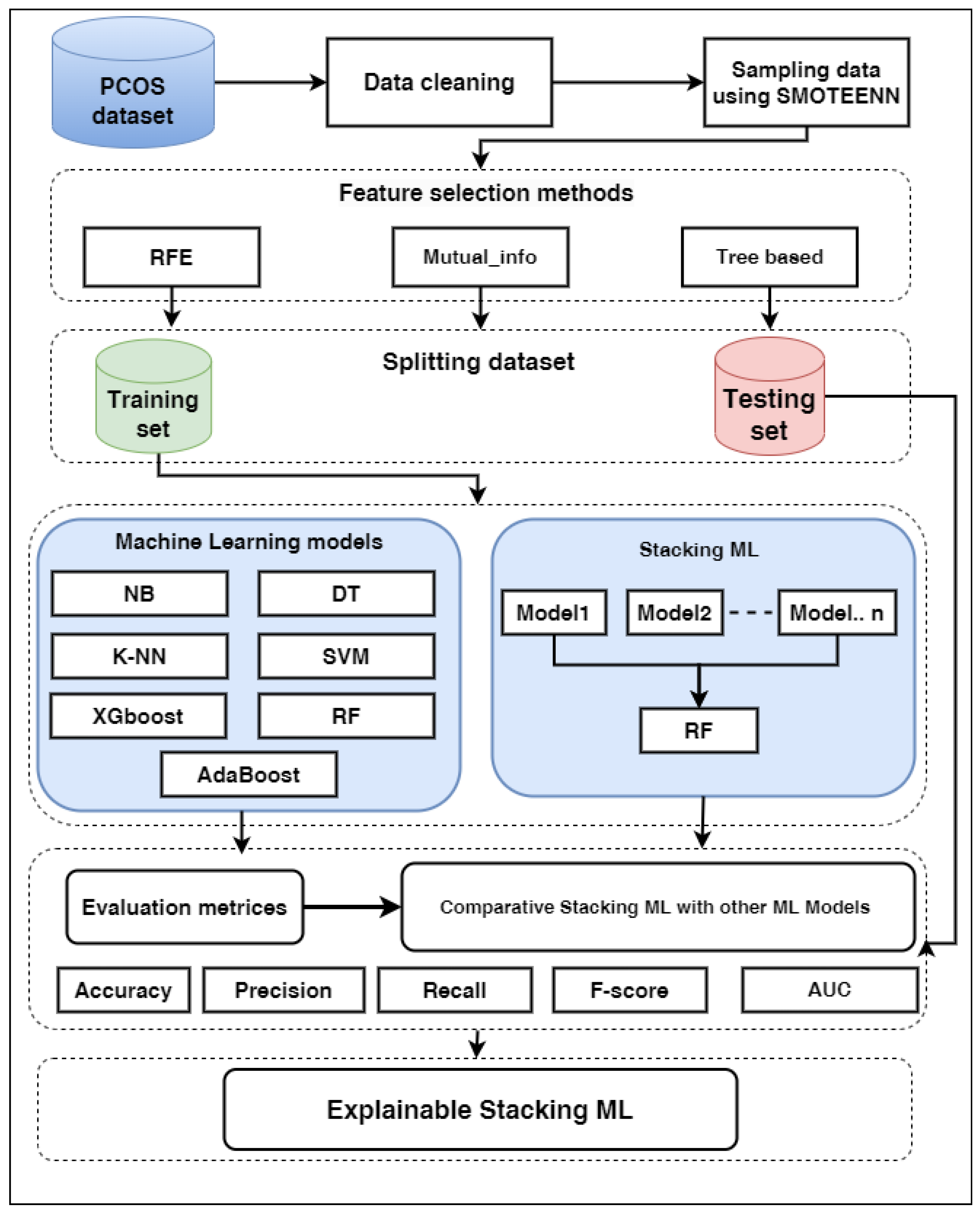
3. Methodology
3.1. Database Description
3.2. Data Processing
Filling Missing Values
3.3. Data Encoding
3.4. Sampling Data
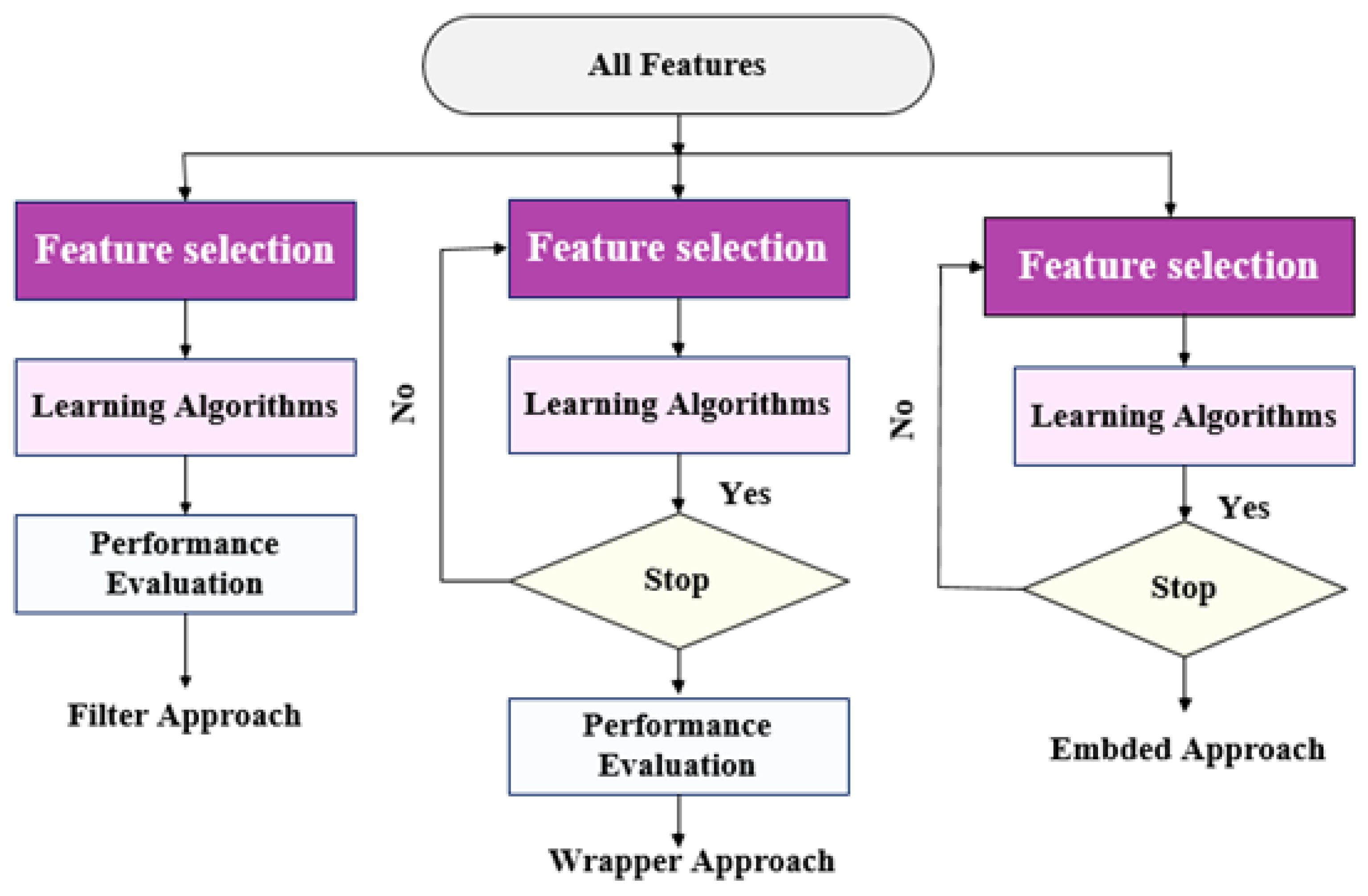
3.5. Feature Selection Techniques
3.5.1. Filter Approach
3.5.2. Wrapper Approach
3.5.3. Embedded Approach
3.6. Splitting Dataset
3.7. Models Optimization and Training
3.7.1. ML Models
3.7.2. Bayesian Optimization
3.8. Stacking Machine Learning
3.9. Evaluating Models
4. Experimental Results
4.1. Experiment Setup
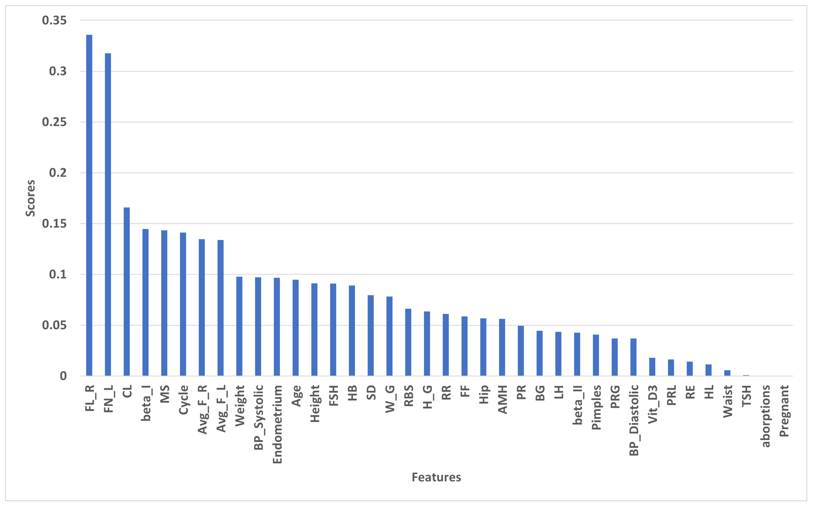
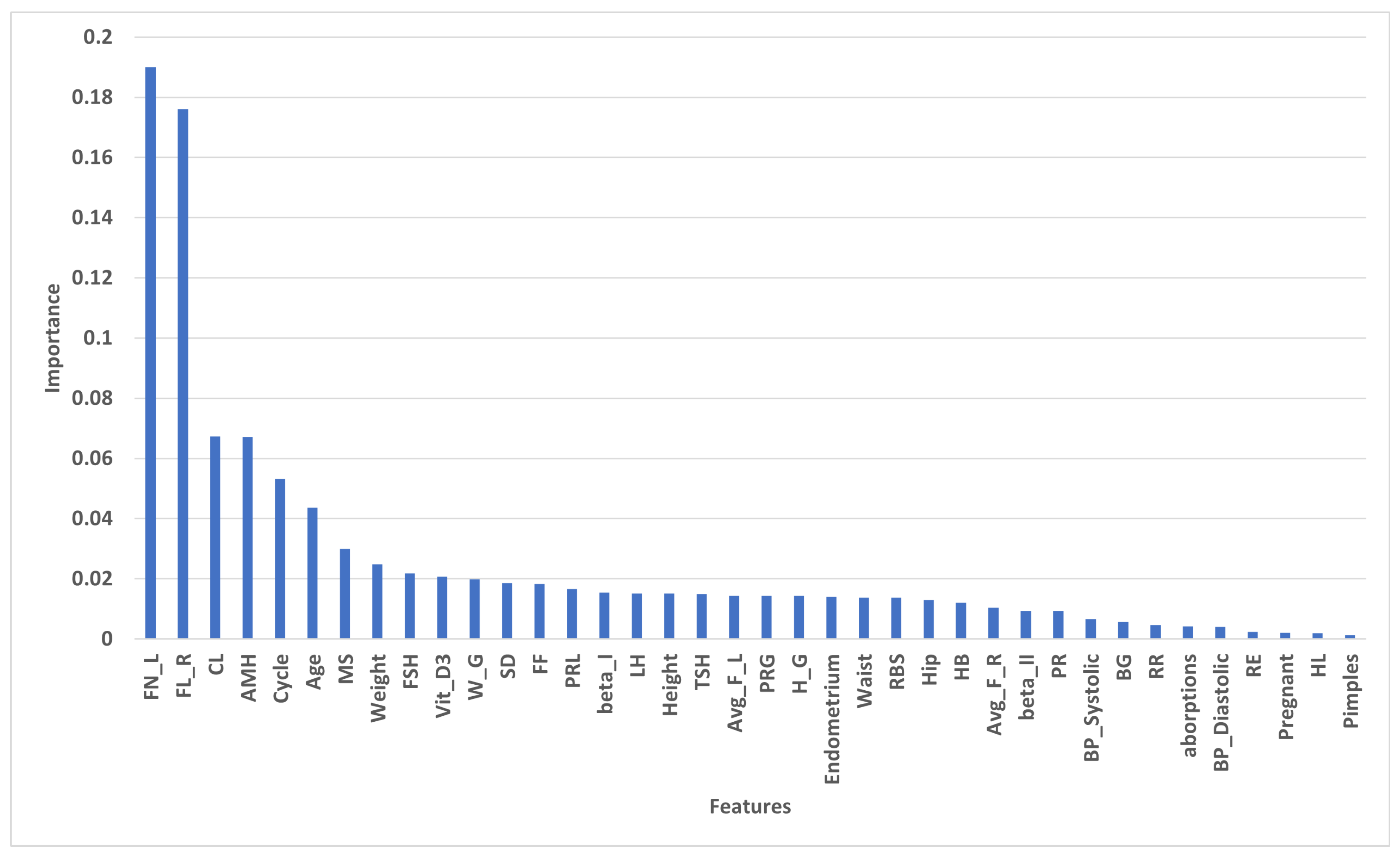
4.2. Feature Selection Methods
4.2.1. Scores of Selected Features by Mutual_Info
4.2.2. Importance of Selected Features by Tree Based
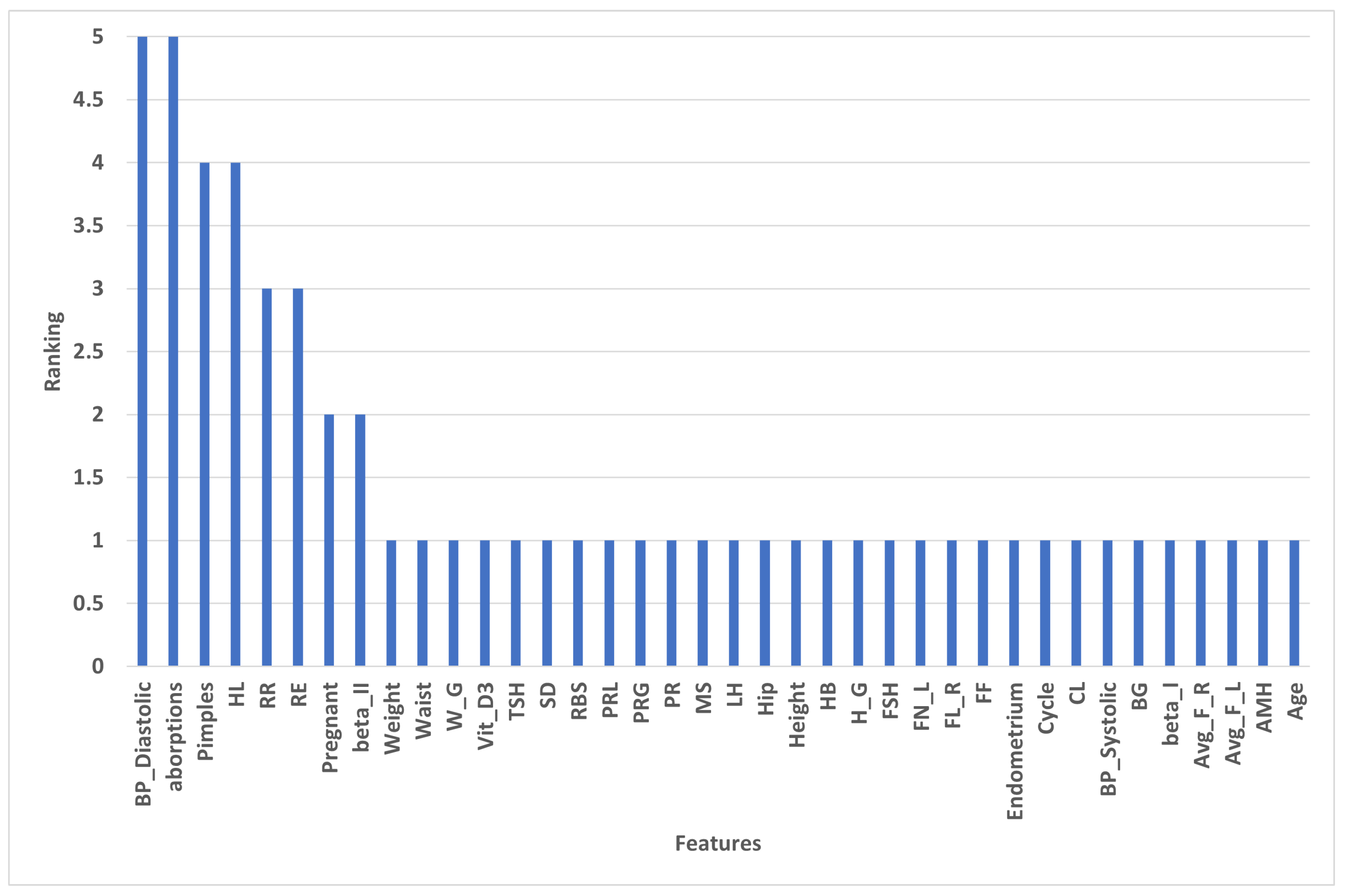
4.2.3. Ranking of Selected Features by RFE
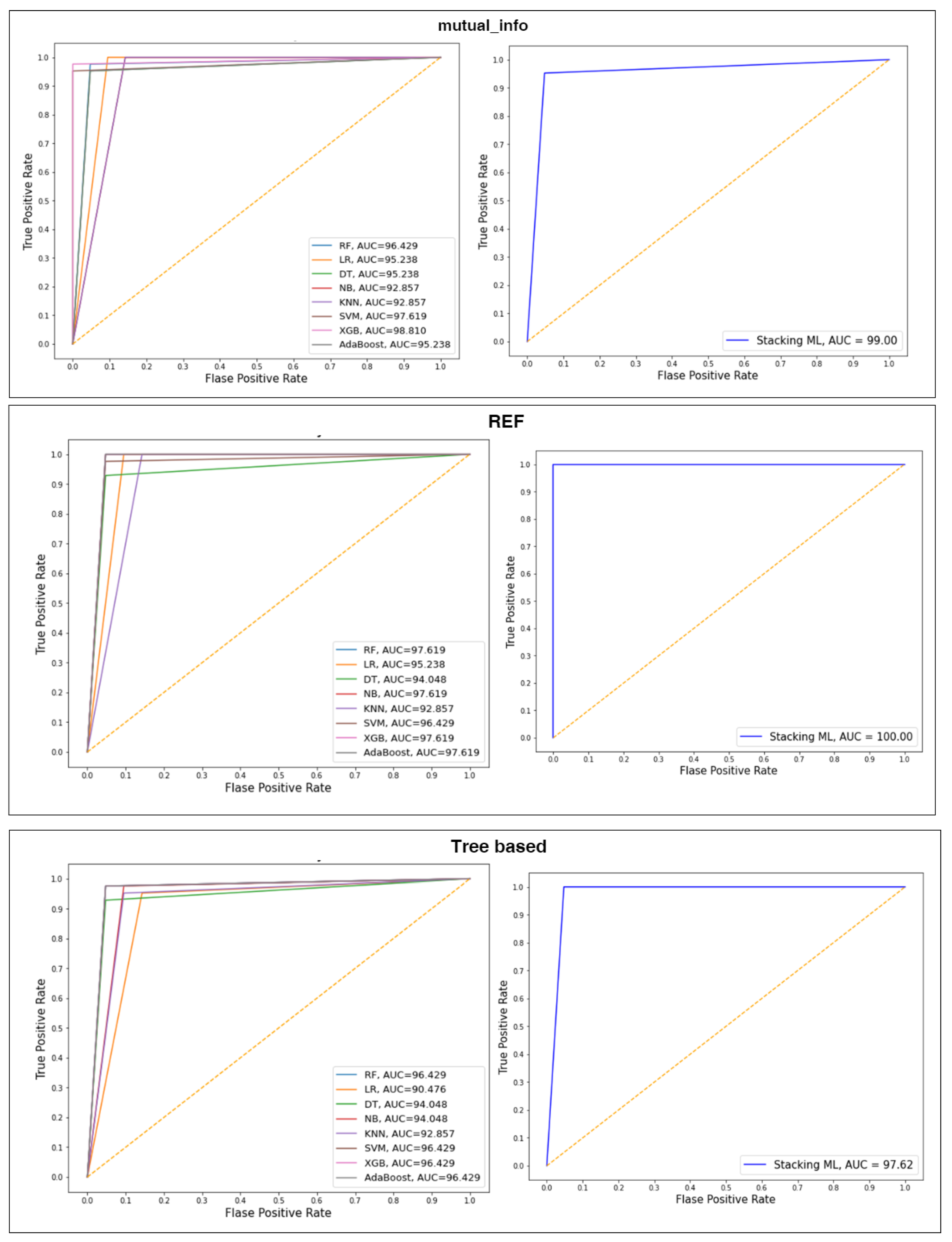
4.3. Performance of the Classifiers with Selected Features Using Splitting 80:20
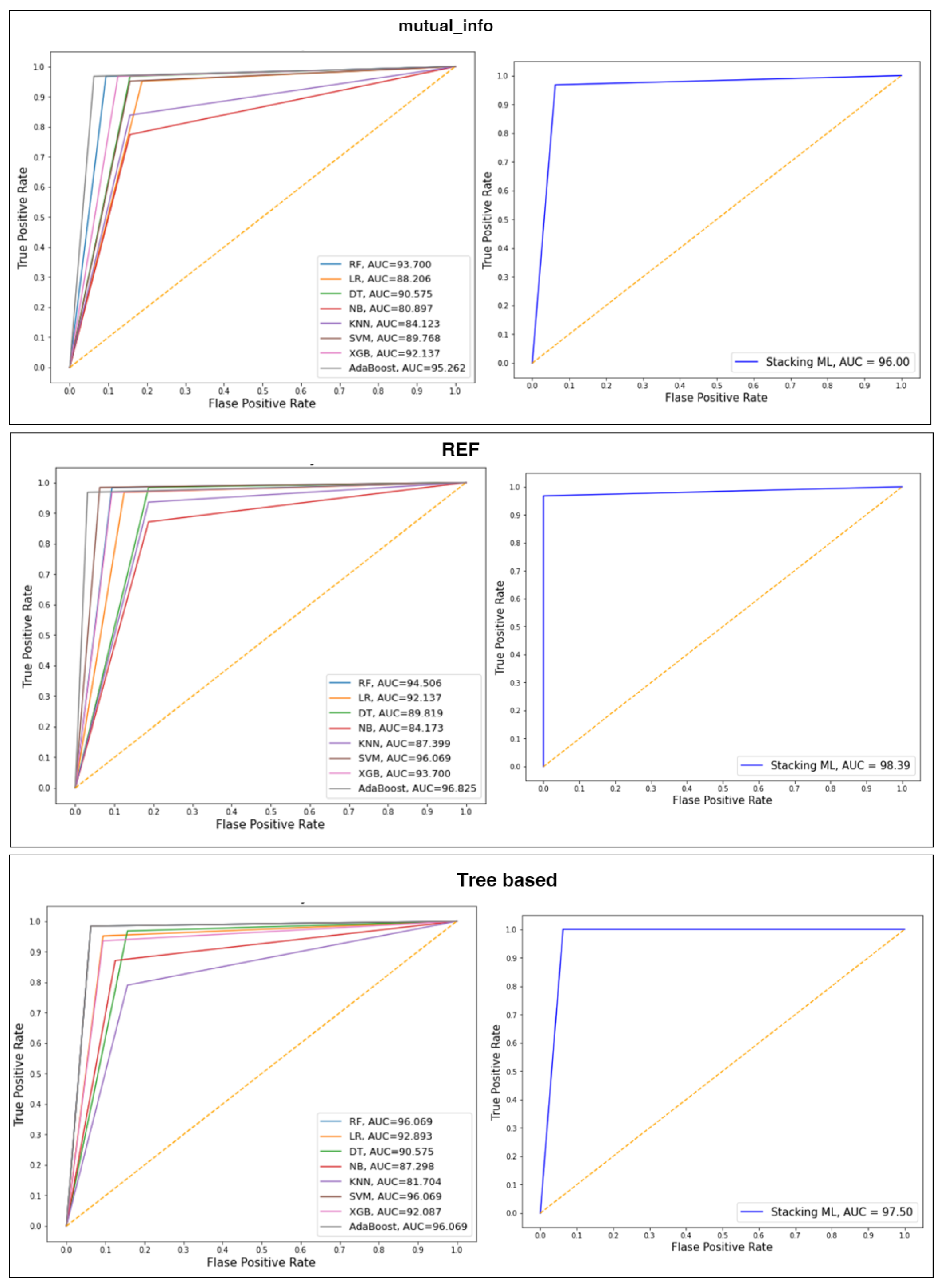
4.4. Performance of the Classifiers with Selected Features Using Splitting 70:30
5. Discussion
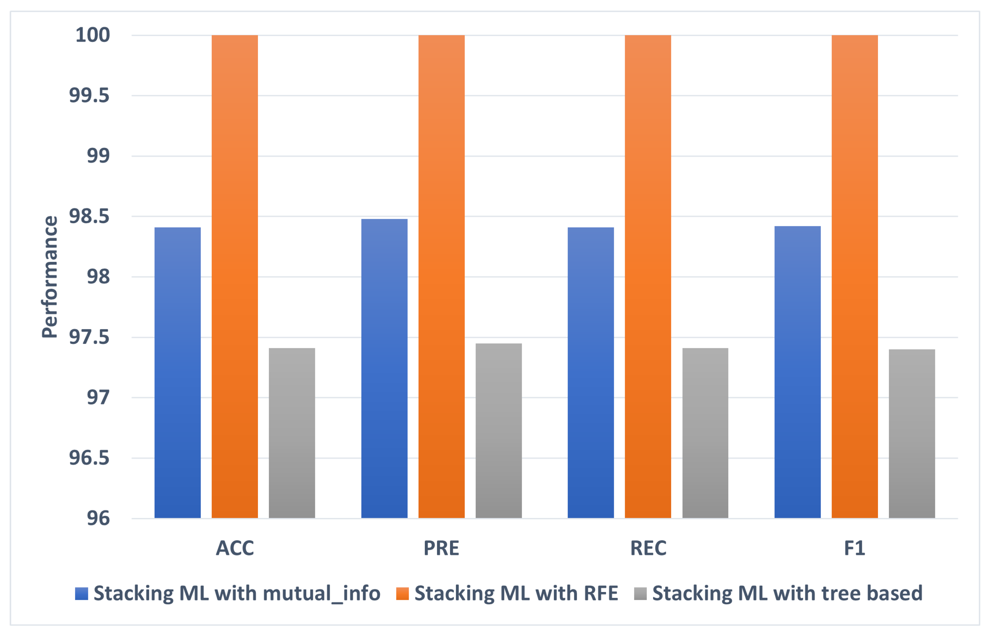
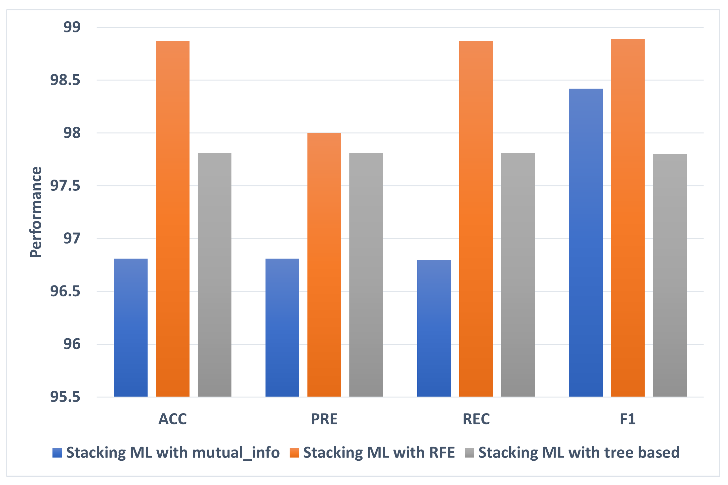
5.1. The Best Models
5.2. Comparison with Previous Studies
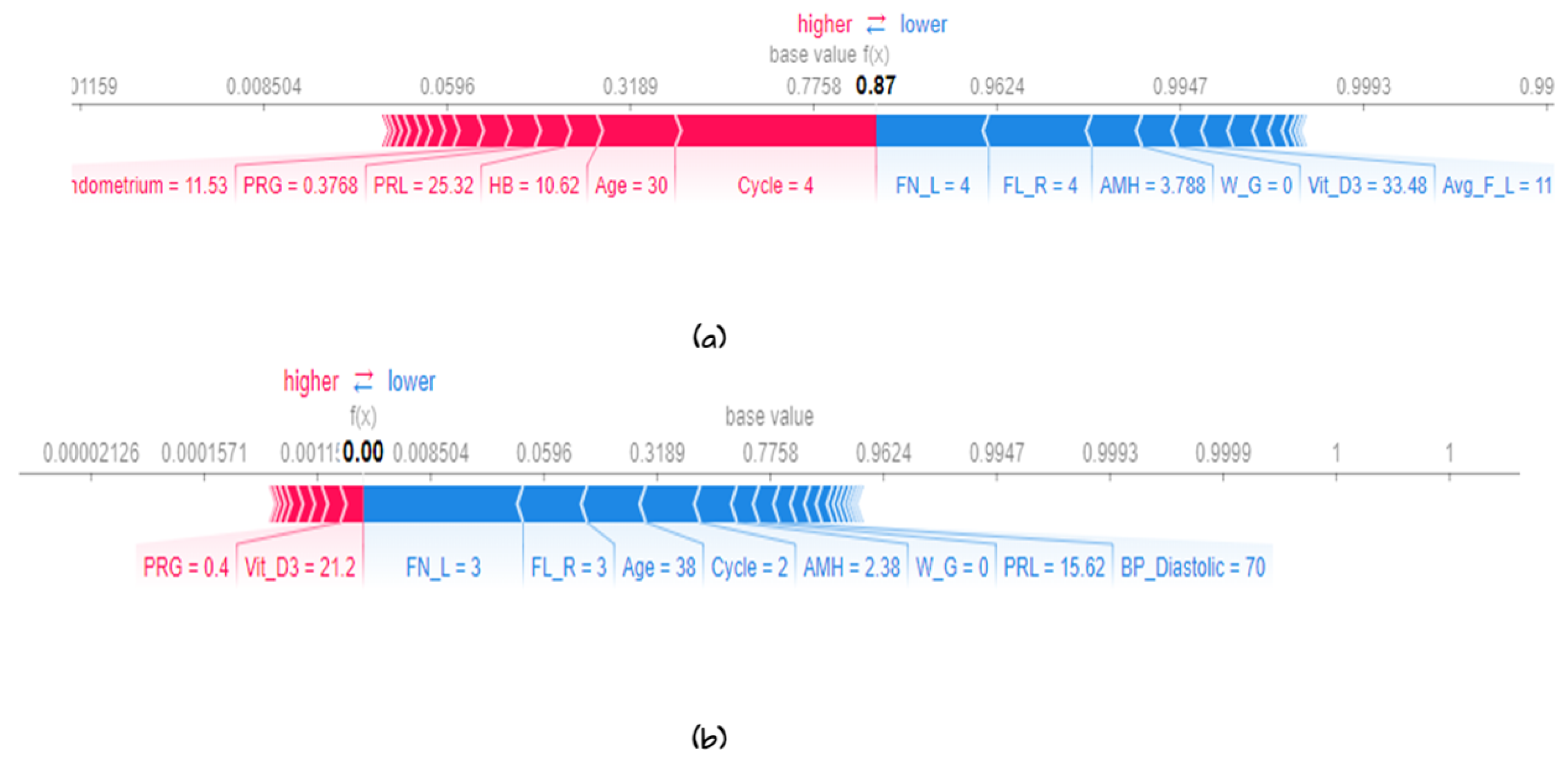
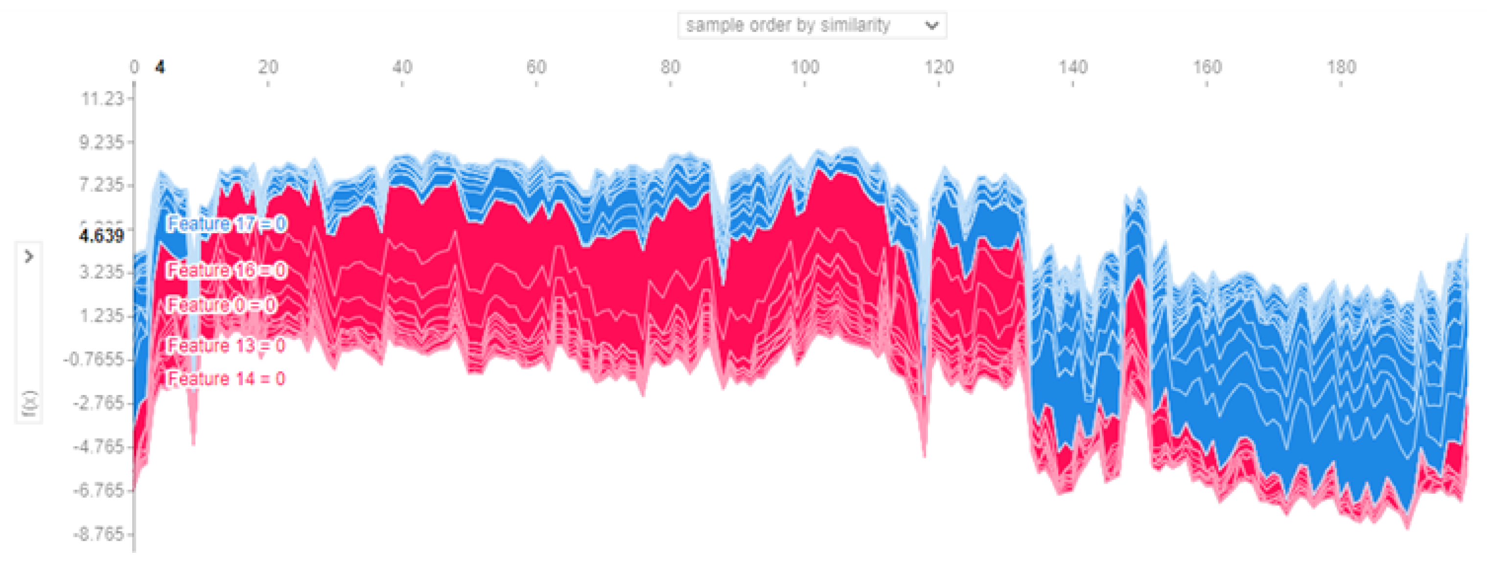
5.3. Model Explainability
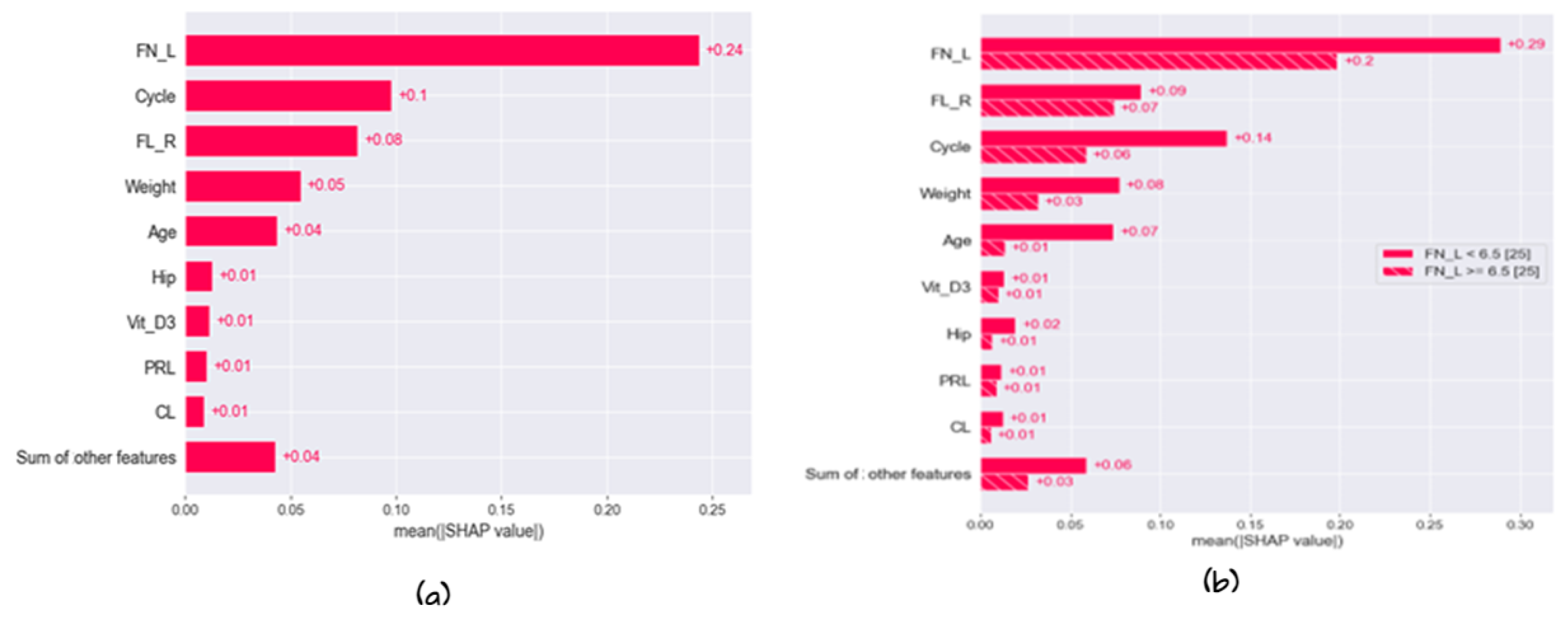
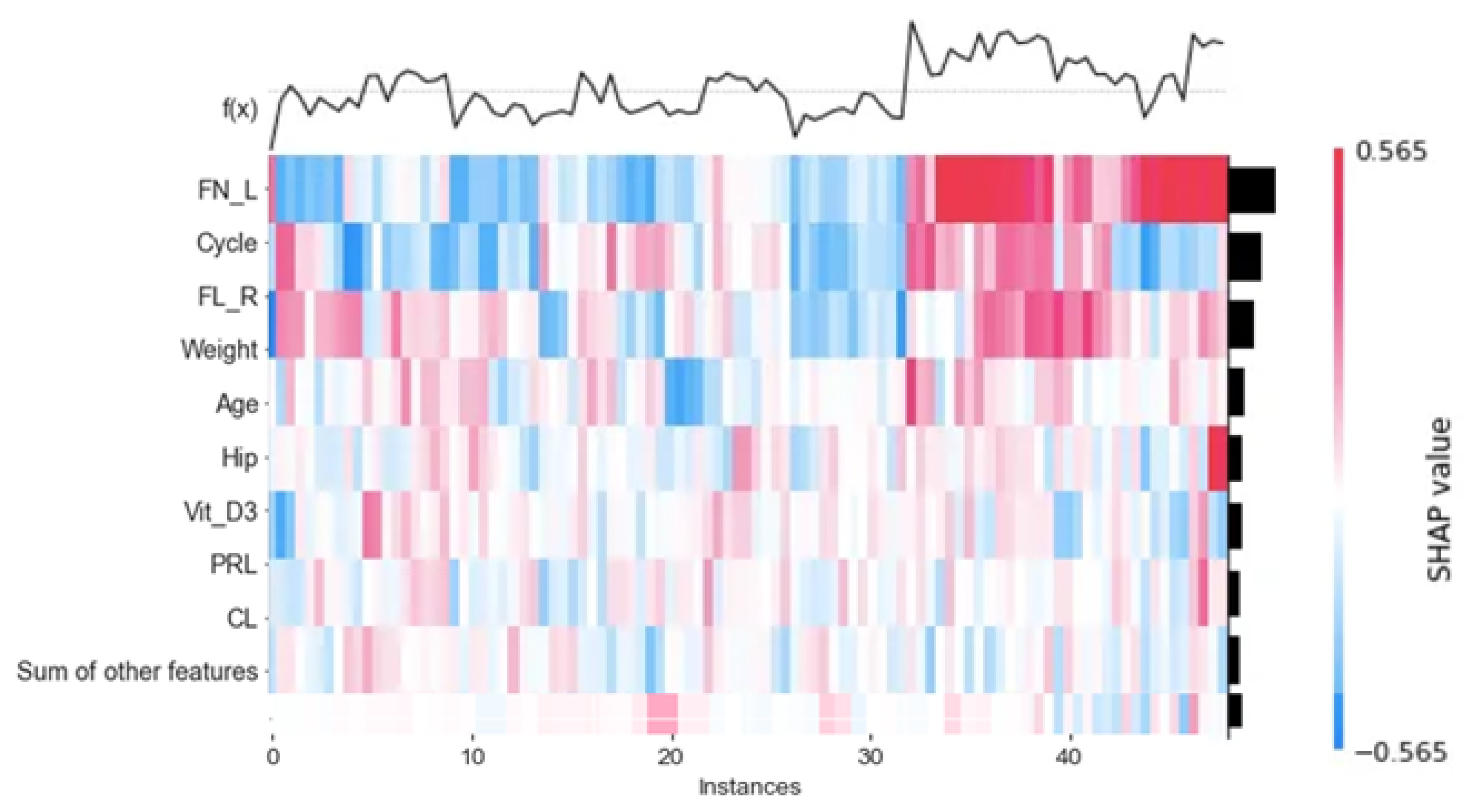
5.3.1. Global Explainability
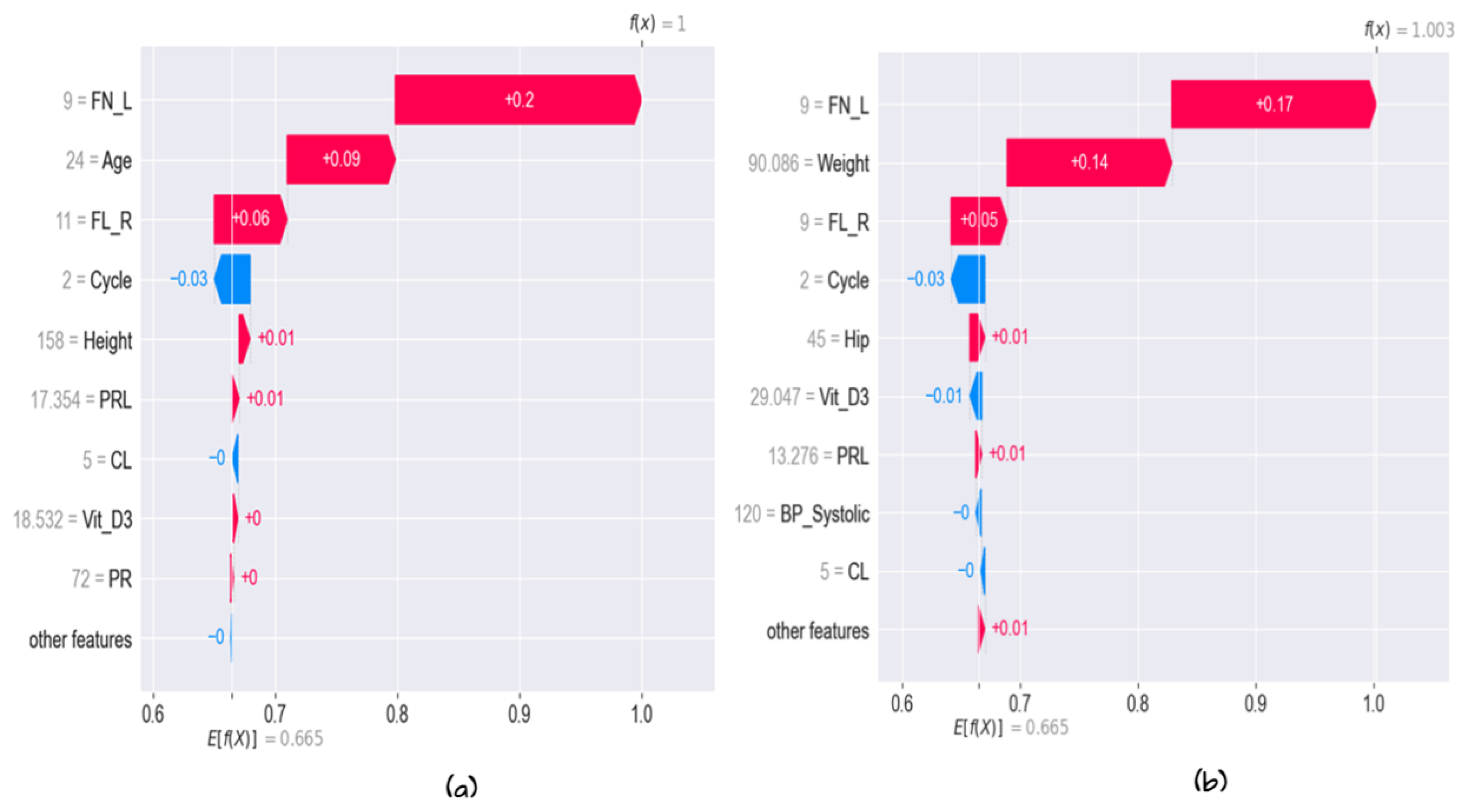
5.3.2. Local Explainability
6. Conclusions
Author Contributions
Funding
Data Availability Statement
Acknowledgments
Conflicts of Interest
References
- Escobar-Morreale, H.F. Polycystic ovary syndrome: Definition, aetiology, diagnosis and treatment. Nat. Rev. Endocrinol. 2018, 14, 270–284. [Google Scholar] [CrossRef] [PubMed]
- Norman, R.J.; Dewailly, D.; Legro, R.S.; Hickey, T.E. Polycystic ovary syndrome. Lancet 2007, 370, 685–697. [Google Scholar] [CrossRef] [PubMed]
- McCartney, C.R.; Marshall, J.C. Polycystic ovary syndrome. N. Engl. J. Med. 2016, 375, 54–64. [Google Scholar] [CrossRef] [PubMed]
- Barber, T.M.; Franks, S. Obesity and polycystic ovary syndrome. Clin. Endocrinol. 2021, 95, 531–541. [Google Scholar] [CrossRef] [PubMed]
- Azziz, R. Polycystic ovary syndrome. Obstet. Gynecol. 2018, 132, 321–336. [Google Scholar] [CrossRef]
- Tiwari, S.; Kane, L.; Koundal, D.; Jain, A.; Alhudhaif, A.; Polat, K.; Zaguia, A.; Alenezi, F.; Althubiti, S.A. SPOSDS: A smart Polycystic Ovary Syndrome diagnostic system using machine learning. Expert Syst. Appl. 2022, 203, 117592. [Google Scholar] [CrossRef]
- Almulihi, A.; Saleh, H.; Hussien, A.M.; Mostafa, S.; El-Sappagh, S.; Alnowaiser, K.; Ali, A.A.; Refaat Hassan, M. Ensemble Learning Based on Hybrid Deep Learning Model for Heart Disease Early Prediction. Diagnostics 2022, 12, 3215. [Google Scholar] [CrossRef]
- Elmannai, H.; Saleh, H.; Algarni, A.D.; Mashal, I.; Kwak, K.S.; El-Sappagh, S.; Mostafa, S. Diagnosis Myocardial Infarction Based on Stacking Ensemble of Convolutional Neural Network. Electronics 2022, 11, 3976. [Google Scholar] [CrossRef]
- Venkatesh, B.; Anuradha, J. A review of feature selection and its methods. Cybern. Inf. Technol. 2019, 19, 3–26. [Google Scholar] [CrossRef]
- Cai, J.; Luo, J.; Wang, S.; Yang, S. Feature selection in machine learning: A new perspective. Neurocomputing 2018, 300, 70–79. [Google Scholar] [CrossRef]
- Sarkar, B.K. Hybrid model for prediction of heart disease. Soft Comput. 2020, 24, 1903–1925. [Google Scholar] [CrossRef]
- Thomas, N.; Kavitha, A. Prediction of polycystic ovarian syndrome with clinical dataset using a novel hybrid data mining classification technique. Int. J. Adv. Res. Eng. Technol. 2020, 11, 1872–1881. [Google Scholar]
- Rudin, C. Stop explaining black box machine learning models for high stakes decisions and use interpretable models instead. Nat. Mach. Intell. 2019, 1, 206–215. [Google Scholar] [CrossRef] [PubMed]
- El-Sappagh, S.; Alonso, J.M.; Islam, S.; Sultan, A.M.; Kwak, K.S. A multilayer multimodal detection and prediction model based on explainable artificial intelligence for Alzheimer’s disease. Sci. Rep. 2021, 11, 2660. [Google Scholar] [CrossRef] [PubMed]
- Lee, H.; Yune, S.; Mansouri, M.; Kim, M.; Tajmir, S.H.; Guerrier, C.E.; Ebert, S.A.; Pomerantz, S.R.; Romero, J.M.; Kamalian, S.; et al. An explainable deep-learning algorithm for the detection of acute intracranial haemorrhage from small datasets. Nat. Biomed. Eng. 2019, 3, 173–182. [Google Scholar] [CrossRef] [PubMed]
- Bharati, S.; Podder, P.; Mondal, M.R.H. Diagnosis of polycystic ovary syndrome using machine learning algorithms. In Proceedings of the 2020 IEEE Region 10 Symposium (TENSYMP), Dhaka, Bangladesh, 5–7 June 2020; pp. 1486–1489. [Google Scholar]
- Denny, A.; Raj, A.; Ashok, A.; Ram, C.M.; George, R. i-hope: Detection and prediction system for polycystic ovary syndrome (pcos) using machine learning techniques. In Proceedings of the TENCON 2019—2019 IEEE Region 10 Conference (TENCON), Kochi, India, 17–20 October 2019; pp. 673–678. [Google Scholar]
- Anda, D.; Iyamah, E. Comparative Analysis of Artificial Intelligence in the Diagnosis of Polycystic Ovary Syndrome. Available online: https://www.researchgate.net/publication/366320486_Comparative_Analysis_of_Artificial_Intelligence_in_the_Diagnosis_of_Polycystic_Ovary_Syndrome (accessed on 17 March 2023).
- Bhardwaj, P.; Tiwari, P. Manoeuvre of Machine Learning Algorithms in Healthcare Sector with Application to Polycystic Ovarian Syndrome Diagnosis. In Proceedings of Academia-Industry Consortium for Data Science: AICDS 2020; Springer: New York, NY, USA, 2022; pp. 71–84. [Google Scholar]
- Adla, Y.A.A.; Raydan, D.G.; Charaf, M.Z.J.; Saad, R.A.; Nasreddine, J.; Diab, M.O. Automated detection of polycystic ovary syndrome using machine learning techniques. In Proceedings of the 2021 Sixth International Conference on Advances in Biomedical Engineering (ICABME), Werdanyeh, Lebanon, 7–9 October 2021; pp. 208–212. [Google Scholar]
- Thakre, V.; Vedpathak, S.; Thakre, K.; Sonawani, S. PCOcare: PCOS detection and prediction using machine learning algorithms. Biosci. Biotechnol. Res. Commun. 2020, 13, 240–244. [Google Scholar] [CrossRef]
- Chauhan, P.; Patil, P.; Rane, N.; Raundale, P.; Kanakia, H. Comparative analysis of machine learning algorithms for prediction of pcos. In Proceedings of the 2021 International Conference on Communication information and Computing Technology (ICCICT), Mumbai, India, 25–27 June 2021; pp. 1–7. [Google Scholar]
- Rathod, Y.; Komare, A.; Ajgaonkar, R.; Chindarkar, S.; Nagare, G.; Punjabi, N.; Karpate, Y. Predictive Analysis of Polycystic Ovarian Syndrome using CatBoost Algorithm. In Proceedings of the 2022 IEEE Region 10 Symposium (TENSYMP), Mumbai, India, 1–3 July 2022; pp. 1–6. [Google Scholar]
- Aggarwal, N.; Shukla, U.; Saxena, G.J.; Kumar, M.; Bafila, A.S.; Singh, S.; Pundir, A. An Improved Technique for Risk Prediction of Polycystic Ovary Syndrome (PCOS) Using Feature Selection and Machine Learning. In Computational Intelligence: Select Proceedings of InCITe 2022; Springer: New York, NY, USA, 2023; pp. 597–606. [Google Scholar]
- Khanna, V.V.; Chadaga, K.; Sampathila, N.; Prabhu, S.; Bhandage, V.; Hegde, G.K. A Distinctive Explainable Machine Learning Framework for Detection of Polycystic Ovary Syndrome. Appl. Syst. Innov. 2023, 6, 32. [Google Scholar] [CrossRef]
- Polycystic Ovary Syndrome (PCOS). 2023. Available online: https://www.kaggle.com/datasets/prasoonkottarathil/polycystic-ovary-syndrome-pcos (accessed on 17 March 2023).
- Mahdhaoui, A.; Chetouani, M.; Cassel, R.S.; Saint-Georges, C.; Parlato, E.; Laznik, M.C.; Apicella, F.; Muratori, F.; Maestro, S.; Cohen, D. Computerized home video detection for motherese may help to study impaired interaction between infants who become autistic and their parents. Int. J. Methods Psychiatr. Res. 2011, 20, e6–e18. [Google Scholar] [CrossRef]
- Joenssen, D.; Bankhofer, U. Hot Deck Methods for Imputing Missing Data Hot Deck Methods for Imputing Missing Data the Effects of Limiting Donor Usage. 13 July 2012. Available online: https://www.semanticscholar.org/paper/Hot-Deck-Methods-for-Imputing-Missing-Data-The-of-Joenssen-Bankhofer/853253faf9d7ee66a4ebd749659c463cdc475f7c (accessed on 17 March 2023).
- Moon, T.K. The expectation-maximization algorithm. IEEE Signal Process. Mag. 1996, 13, 47–60. [Google Scholar] [CrossRef]
- Cho, E.; Chang, T.W.; Hwang, G. Data preprocessing combination to improve the performance of quality classification in the manufacturing process. Electronics 2022, 11, 477. [Google Scholar] [CrossRef]
- Gu, Q.; Li, Z.; Han, J. Generalized fisher score for feature selection. arXiv 2012, arXiv:1202.3725. [Google Scholar]
- Lin, X.; Li, C.; Zhang, Y.; Su, B.; Fan, M.; Wei, H. Selecting feature subsets based on SVM-RFE and the overlapping ratio with applications in bioinformatics. Molecules 2017, 23, 52. [Google Scholar] [CrossRef] [PubMed]
- Huang, J.; Cai, Y.; Xu, X. A filter approach to feature selection based on mutual information. In Proceedings of the 2006 5th IEEE International Conference on Cognitive Informatics, Beijing, China, 17–19 July 2006; Volume 1, pp. 84–89. [Google Scholar]
- He, Y.; Yu, H.; Yu, R.; Song, J.; Lian, H.; He, J.; Yuan, J. A correlation-based feature selection algorithm for operating data of nuclear power plants. Sci. Technol. Nucl. Install. 2021, 2021, 9994340. [Google Scholar] [CrossRef]
- Bateni, M.; Chen, L.; Fahrbach, M.; Fu, G.; Mirrokni, V.; Yasuda, T. Sequential Attention for Feature Selection. arXiv 2022, arXiv:2209.14881. [Google Scholar]
- Socher, R.; Perelygin, A.; Wu, J.; Chuang, J.; Manning, C.D.; Ng, A.Y.; Potts, C. Recursive deep models for semantic compositionality over a sentiment treebank. In Proceedings of the 2013 Conference on Empirical Methods in Natural Language Processing, Seattle, WA, USA, 18–21 October 2013; pp. 1631–1642. [Google Scholar]
- LaValley, M.P. Logistic regression. Circulation 2008, 117, 2395–2399. [Google Scholar] [CrossRef] [PubMed]
- Rigatti, S.J. Random forest. J. Insur. Med. 2017, 47, 31–39. [Google Scholar] [CrossRef] [PubMed]
- Webb, G.I.; Keogh, E.; Miikkulainen, R. Naïve Bayes. Encycl. Mach. Learn. 2010, 15, 713–714. [Google Scholar]
- Suthaharan, S.; Suthaharan, S. Support vector machine. In Machine Learning Models and Algorithms for Big Data Classification: Thinking with Examples for Effective Learning; Spring: Berlin/Heidelberg, Germany, 2016; pp. 207–235. [Google Scholar]
- Peterson, L.E. K-nearest neighbor. Scholarpedia 2009, 4, 1883. [Google Scholar] [CrossRef]
- Chen, T.; He, T.; Benesty, M.; Khotilovich, V.; Tang, Y.; Cho, H.; Chen, K.; Mitchell, R.; Cano, I.; Zhou, T.; et al. Xgboost: Extreme Gradient Boosting. R Package Version 0.4-2. 2015, Volume 1, pp. 1–4. Available online: https://scholar.google.com/scholar?oi=bibs&cluster=11444560539169478279&btnI=1&hl=en (accessed on 17 March 2023).
- Schapire, R.E. Explaining adaboost. In Empirical Inference: Festschrift in Honor of Vladimir N. Vapnik; Spring: Berlin/Heidelberg, Germany, 2013; pp. 37–52. [Google Scholar]
- Wu, J.; Chen, X.Y.; Zhang, H.; Xiong, L.D.; Lei, H.; Deng, S.H. Hyperparameter optimization for machine learning models based on Bayesian optimization. J. Electron. Sci. Technol. 2019, 17, 26–40. [Google Scholar]
- Snoek, J.; Larochelle, H.; Adams, R.P. Practical bayesian optimization of machine learning algorithms. In Proceedings of the Advances in Neural Information Processing Systems, Lake Tahoe, NV, USA, 3–6 December 2012; Volume 25. [Google Scholar]
- El-Rashidy, N.; Abuhmed, T.; Alarabi, L.; El-Bakry, H.M.; Abdelrazek, S.; Ali, F.; El-Sappagh, S. Sepsis prediction in intensive care unit based on genetic feature optimization and stacked deep ensemble learning. In Neural Computing and Applications; Spring: Berlin/Heidelberg, Germany, 2022; pp. 1–30. [Google Scholar]
- Saleh, H.; Mostafa, S.; Alharbi, A.; El-Sappagh, S.; Alkhalifah, T. Heterogeneous ensemble deep learning model for enhanced Arabic sentiment analysis. Sensors 2022, 22, 3707. [Google Scholar] [CrossRef]
- El-Rashidy, N.; El-Sappagh, S.; Abuhmed, T.; Abdelrazek, S.; El-Bakry, H.M. Intensive care unit mortality prediction: An improved patient-specific stacking ensemble model. IEEE Access 2020, 8, 133541–133564. [Google Scholar] [CrossRef]
- Narkhede, S. Understanding auc-roc curve. Towards Data Sci. 2018, 26, 220–227. [Google Scholar]


| Feature Name | Abb | Description |
|---|---|---|
| Patient File No. | Patient file number (unique identifier) | |
| Polycystic Ovary Syndrome | PCOS | Class label (determine if the patient has this syndrome or not) |
| Age | AGE | Patient’s age in years |
| Weight | WEIGHT | Patient’s weight in KG |
| Height | HEIGHT | Patient’s height in CM |
| Body Mass Index | BMI | Body mass index of the patient (height/weight) |
| Blood Group | BG | Patients belong to which blood group (A+, A−, B+, B−, O+, O−, AB+, AB−) |
| Pulse Rate | PR | Heartbeat per minute |
| Respiration Rates | RR | Respiration rates per minute |
| Hemoglobin | HB | Number of red blood cells in patient’s body |
| Cycle | CYCLE | Length of the menstrual cycle |
| Cycle Length | CL | Number of days of a cycle |
| Marriage Status | MS | Number of years since marriage |
| Pregnant | P | Pregnant status |
| No. of Abortions | AB | No. of abortions |
| I Beta-HCG | BETA_I | Amount of human chorionic gonadotropin |
| Beta Healthy Singleton Pregnancy | BETA_II | Beta HCG level is indication of 100 mIU/ml about 16 days after ovulation, |
| Follicle-Stimulating Hormone | FSH | Attributes ranging from 0.3 to 10.0 mIU/mL indicate if are still menstruating or have undergone menopause |
| Luteinizing Hormone | LH | Chemical agitator that stimulates the reproductive system |
| Follicle-Stimulating Hormone/ Luteinizing Hormone | FSH/LH | Ratio of FSH and LH |
| Hip Size | HIP | Size of hip in inches |
| Waist Size | WAIST | Size of waist in inches |
| Waist-Hip Ratio | HIP_RATIO | Waist size proportion to hip |
| Thyroid-Stimulating Hormone | TSH | Amount of TSH in the blood |
| Anti-Mullerian Hormone | AMH | Plays a key role in developing a baby’s sex organs while in the womb |
| Prolactin levels | PRL | Prolactin levels in women’s bodies |
| Vitamin D | VIT_D3 | Vitamin D levels |
| Progesterone Levels | PRG | Progesterone levels |
| Random Blood Sugar | RBS | Value of random blood sugar (RBS) test |
| Weight Gain | WG | Test to check if the patient gains weight |
| Hair Growth | HG | Test to check if a patient has hair growth |
| Skin Darkening | SD | Test to check the appearance of darkness in skin |
| Hair Loss | HL | Test to check hair loss |
| Pimples | PIMPLES | Pimple issues |
| Fast Food | FF | Check if fast food part of the diet |
| Reg.Exercise | RE | Check if patient exercises on a regular basis |
| Blood Pressure Systolic | BP_ SYSTOLIC: | Amount of pressure in the arteries when the heart is contracting |
| Blood Pressure Diastolic | BP_ Diastolic | Amount of pressure in the arteries while the heart is resting in between heart beats |
| Follicle No. | FN | Follicle number in the left side |
| Feature Selection Methods | Models | ACC | PRE | REC | F1 |
|---|---|---|---|---|---|
| mutual_info | RF | 96.83 | 96.83 | 96.83 | 96.83 |
| LR | 96.83 | 96.97 | 96.83 | 96.78 | |
| DT | 95.24 | 95.34 | 95.24 | 95.26 | |
| NB | 95.24 | 95.56 | 95.24 | 95.14 | |
| KNN | 95.24 | 95.56 | 95.24 | 95.14 | |
| SVM | 96.83 | 97.10 | 96.83 | 96.86 | |
| XGB | 98.12 | 98.10 | 98.12 | 98.12 | |
| AdaBoost | 95.24 | 95.34 | 95.24 | 95.26 | |
| Stacking ML | 98.41 | 98.48 | 98.41 | 98.42 | |
| RFE | RF | 98.41 | 98.45 | 98.41 | 98.40 |
| LR | 96.83 | 96.97 | 96.83 | 96.78 | |
| DT | 93.65 | 93.99 | 93.65 | 93.72 | |
| NB | 98.41 | 98.45 | 98.41 | 98.40 | |
| KNN | 95.24 | 95.56 | 95.24 | 95.14 | |
| SVM | 96.83 | 96.83 | 96.83 | 96.83 | |
| XGB | 98.41 | 98.45 | 98.41 | 98.40 | |
| AdaBoost | 98.41 | 98.45 | 98.41 | 98.40 | |
| Stacking ML | 100 | 100 | 100 | 100 | |
| Tree based | RF | 96.83 | 96.83 | 96.83 | 96.83 |
| LR | 92.06 | 92.02 | 92.06 | 92.01 | |
| DT | 93.65 | 93.99 | 93.65 | 93.72 | |
| NB | 95.24 | 95.23 | 95.24 | 95.21 | |
| KNN | 93.65 | 93.65 | 93.65 | 93.65 | |
| SVM | 96.83 | 96.83 | 96.83 | 96.83 | |
| XGB | 96.83 | 96.83 | 96.83 | 96.83 | |
| AdaBoost | 96.83 | 96.83 | 96.83 | 96.83 | |
| Stacking ML | 97.41 | 97.45 | 97.41 | 97.4 |
| Feature Selection Methods | Models | ACC | PRE | REC | F1 |
|---|---|---|---|---|---|
| mutual_info | RF | 94.68 | 94.66 | 94.68 | 94.66 |
| LR | 90.43 | 90.39 | 90.43 | 90.30 | |
| DT | 92.55 | 92.58 | 92.55 | 92.46 | |
| NB | 79.79 | 82.15 | 79.79 | 80.24 | |
| KNN | 84.04 | 85.01 | 84.04 | 84.29 | |
| SVM | 91.49 | 91.44 | 91.49 | 91.42 | |
| XGB | 93.62 | 93.61 | 93.62 | 93.56 | |
| AdaBoost | 95.74 | 95.74 | 95.74 | 95.74 | |
| Stacking ML | 96.81 | 96.81 | 96.81 | 96.80 | |
| RFE | RF | 95.74 | 95.77 | 95.74 | 95.71 |
| LR | 93.62 | 93.61 | 93.62 | 93.56 | |
| DT | 92.55 | 92.83 | 92.55 | 92.38 | |
| NB | 85.11 | 85.39 | 85.11 | 85.21 | |
| KNN | 89.36 | 89.28 | 89.36 | 89.27 | |
| SVM | 96.81 | 96.81 | 96.81 | 96.80 | |
| XGB | 94.68 | 94.66 | 94.68 | 94.66 | |
| AdaBoost | 96.81 | 96.86 | 96.81 | 96.82 | |
| Stacking ML | 98.87 | 98.00 | 98.87 | 98.89 | |
| Tree based | RF | 95.81 | 95.81 | 95.81 | 95.80 |
| LR | 93.62 | 93.62 | 93.62 | 93.62 | |
| DT | 92.55 | 92.58 | 92.55 | 92.46 | |
| NB | 87.23 | 87.89 | 87.23 | 87.40 | |
| KNN | 80.85 | 82.83 | 80.85 | 81.25 | |
| SVM | 96.81 | 96.81 | 96.81 | 96.80 | |
| XGB | 92.55 | 92.63 | 92.55 | 92.58 | |
| AdaBoost | 96.81 | 96.81 | 96.81 | 96.80 | |
| Stacking ML | 97.81 | 97.81 | 97.81 | 97.8 |
| Papers | Methods | Accuracy |
|---|---|---|
| [16] | RFLR with UFS | 91.01 |
| [17] | RF with PCA | 89.02 |
| [6] | RF with correlation | 92.4 |
| [18] | RF | 96 |
| [19] | SVM with Pearson correlation | 93 |
| [20] | SVM with hybrid feature selection | 91.6 |
| [21] | RF with chi square | 90.9 |
| [22] | DT with Gini importance | 92.59 |
| [25] | multi-stack of ML | 98 |
| Our work | Stacking ML with RFE | 100 |
Disclaimer/Publisher’s Note: The statements, opinions and data contained in all publications are solely those of the individual author(s) and contributor(s) and not of MDPI and/or the editor(s). MDPI and/or the editor(s) disclaim responsibility for any injury to people or property resulting from any ideas, methods, instructions or products referred to in the content. |
© 2023 by the authors. Licensee MDPI, Basel, Switzerland. This article is an open access article distributed under the terms and conditions of the Creative Commons Attribution (CC BY) license (https://creativecommons.org/licenses/by/4.0/).
Share and Cite
Elmannai, H.; El-Rashidy, N.; Mashal, I.; Alohali, M.A.; Farag, S.; El-Sappagh, S.; Saleh, H. Polycystic Ovary Syndrome Detection Machine Learning Model Based on Optimized Feature Selection and Explainable Artificial Intelligence. Diagnostics 2023, 13, 1506. https://doi.org/10.3390/diagnostics13081506
Elmannai H, El-Rashidy N, Mashal I, Alohali MA, Farag S, El-Sappagh S, Saleh H. Polycystic Ovary Syndrome Detection Machine Learning Model Based on Optimized Feature Selection and Explainable Artificial Intelligence. Diagnostics. 2023; 13(8):1506. https://doi.org/10.3390/diagnostics13081506
Chicago/Turabian StyleElmannai, Hela, Nora El-Rashidy, Ibrahim Mashal, Manal Abdullah Alohali, Sara Farag, Shaker El-Sappagh, and Hager Saleh. 2023. "Polycystic Ovary Syndrome Detection Machine Learning Model Based on Optimized Feature Selection and Explainable Artificial Intelligence" Diagnostics 13, no. 8: 1506. https://doi.org/10.3390/diagnostics13081506