
Application of Machine Learning in Epileptic Seizure Detection
 , , ,
, , ,
Abstract
:1. Introduction
2. Literature Review
2.1. Related Works
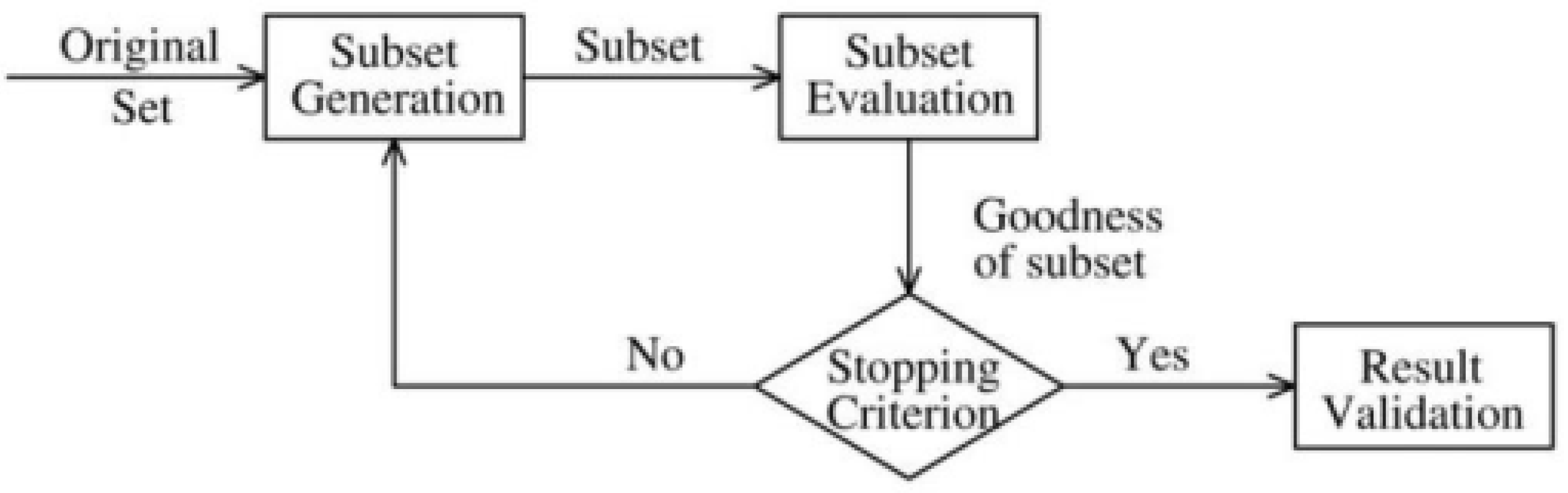
2.2. Feature Selection
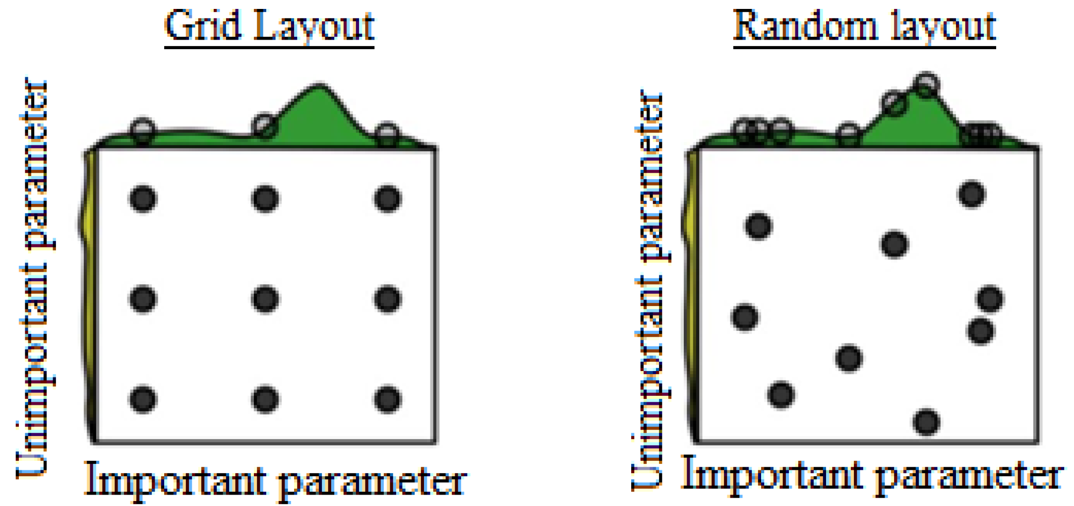
2.3. Hyperparameter Optimization
2.4. Classification
2.4.1. Support Vector Machine (SVM)
2.4.2. K-Nearest Neighbors (KNN)
2.4.3. Decision Tree (DT)
2.4.4. Random Forest (RF)
3. Methodology
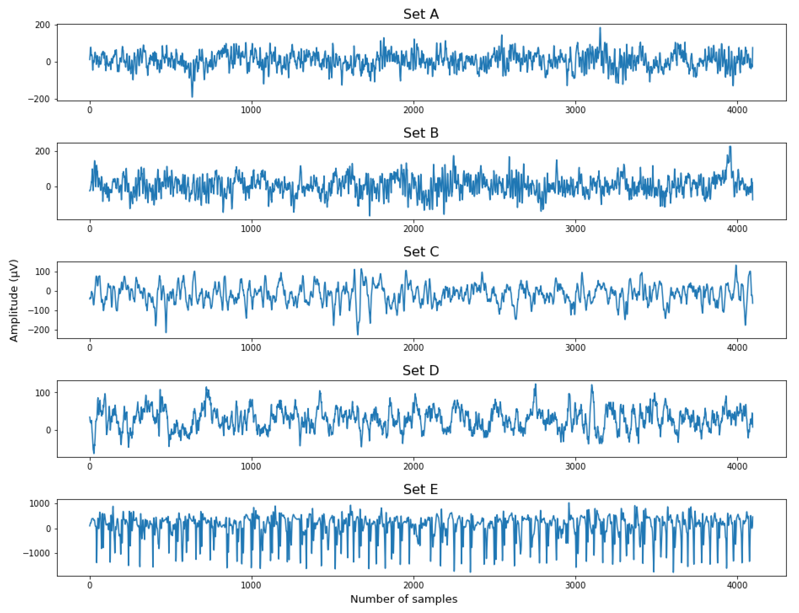
3.1. EEG Dataset from Bonn University
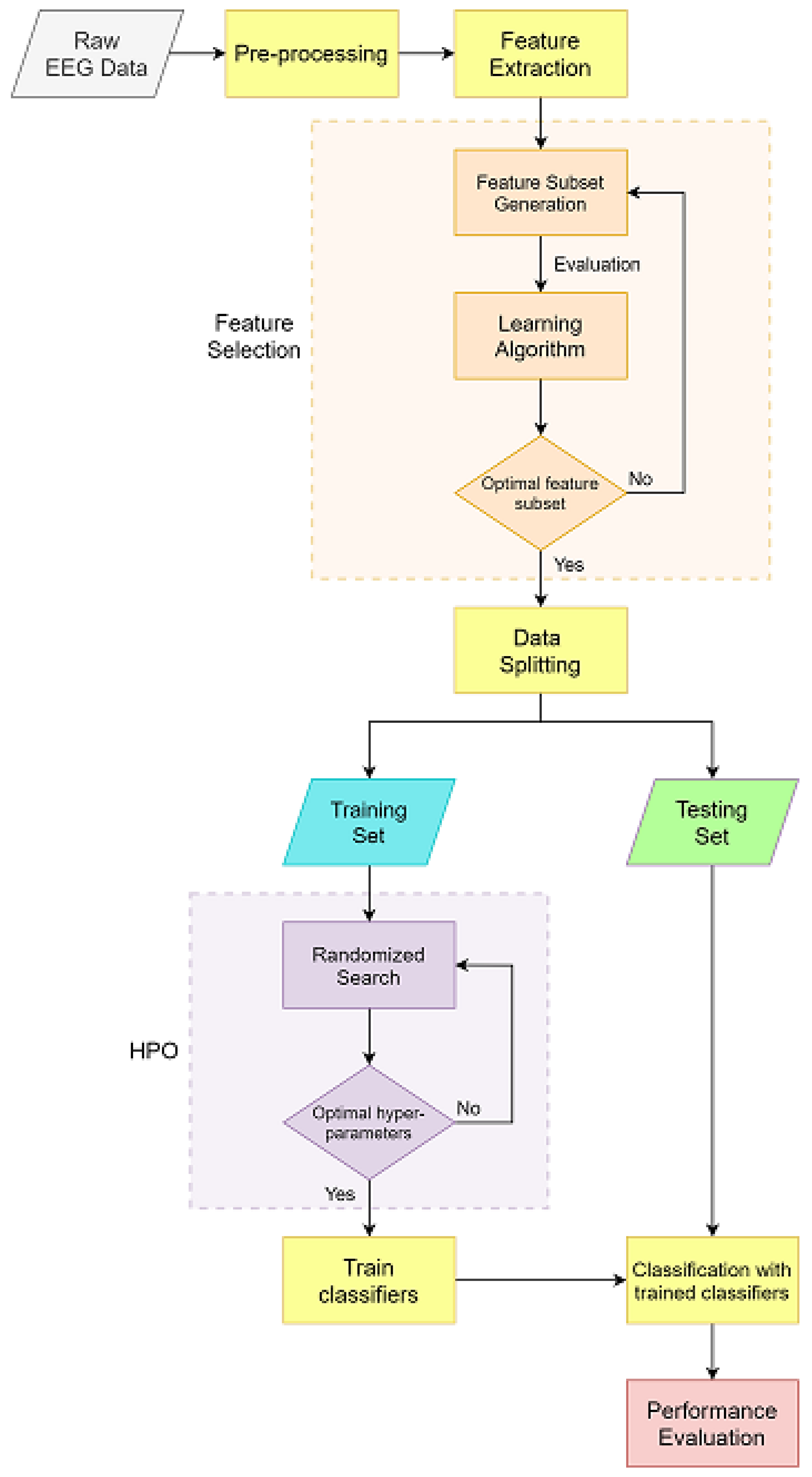
3.2. Model Development
3.2.1. Data Preprocessing
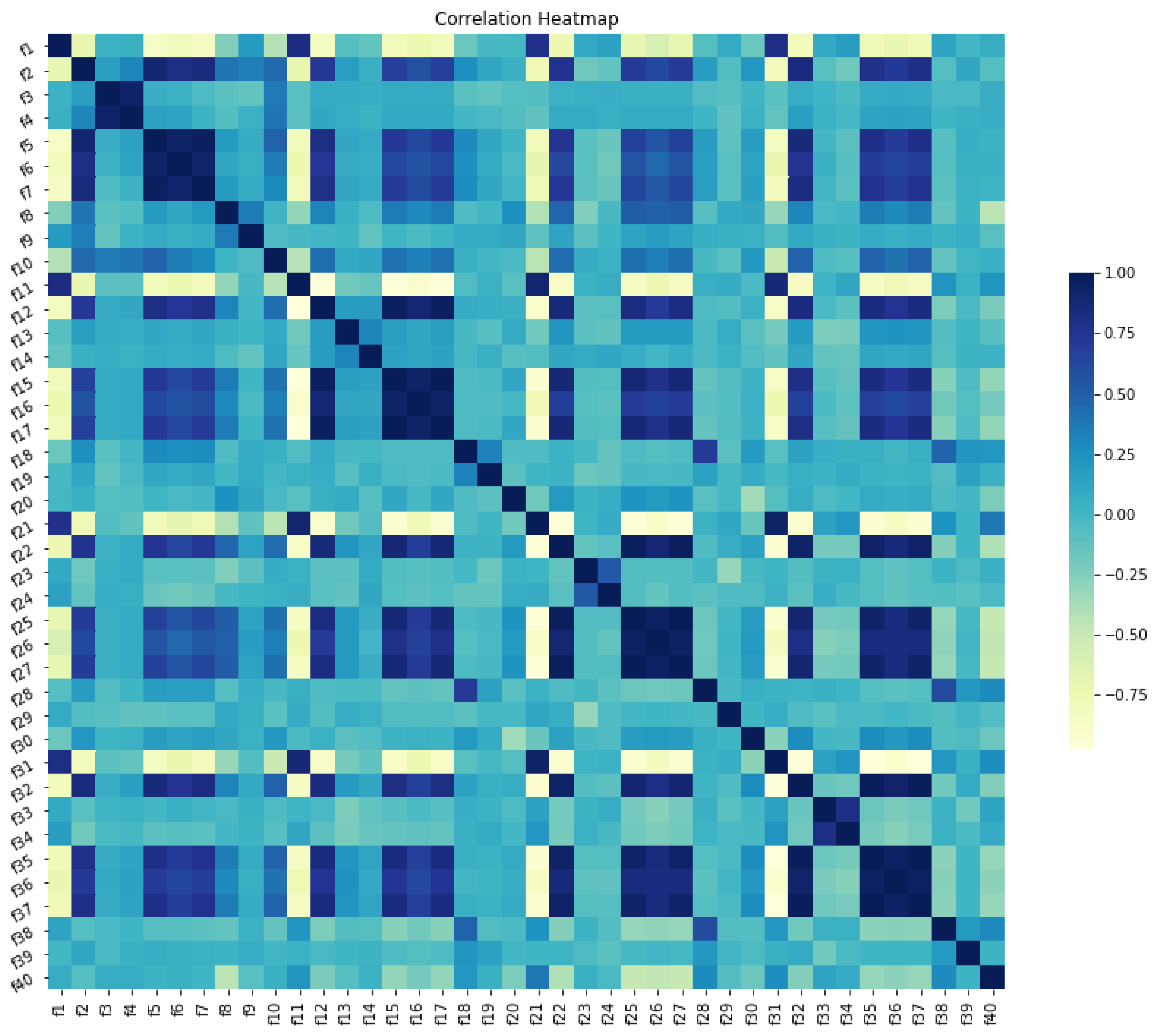
3.2.2. Feature Extraction
3.2.3. Baseline Results
3.3. Model Improvement
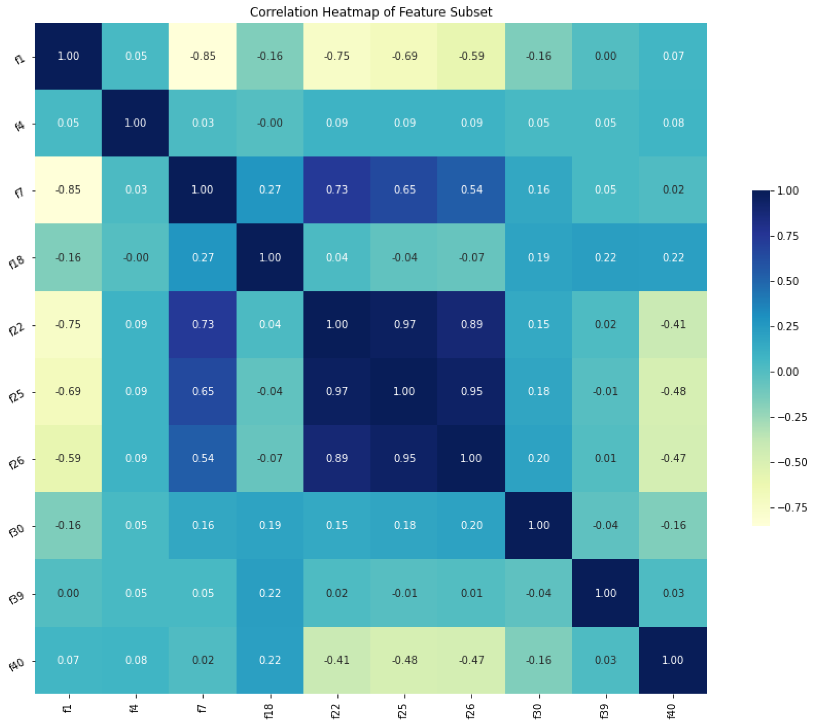
3.3.1. Feature Selection
- Cognitive coefficient c1: 0.7
- Social coefficient c2: 0.7
- Inertia weight w: 0.5
- Number of particles: 40
- Number of neighbors that the particle considers k: 40
3.3.2. Hyperparameter Optimization
4. Experimental Results
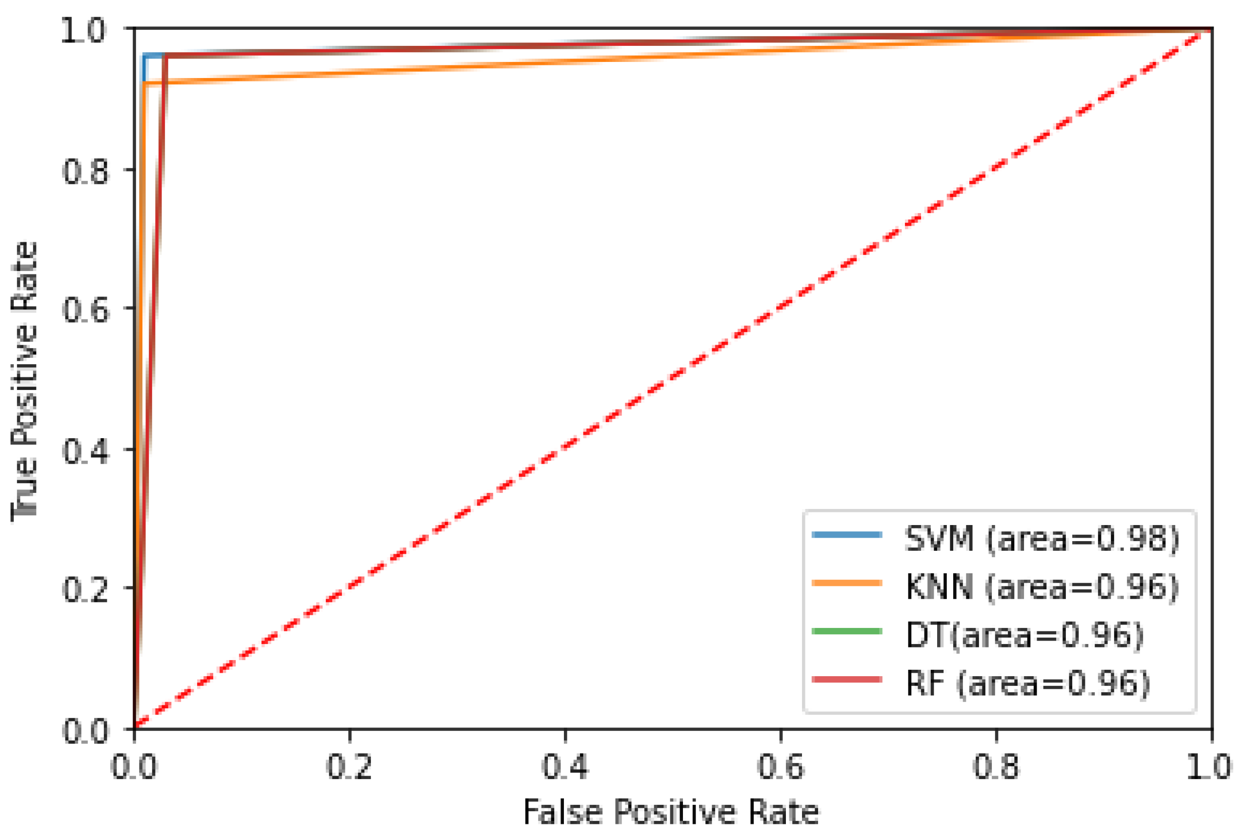
4.1. Performance Evaluation
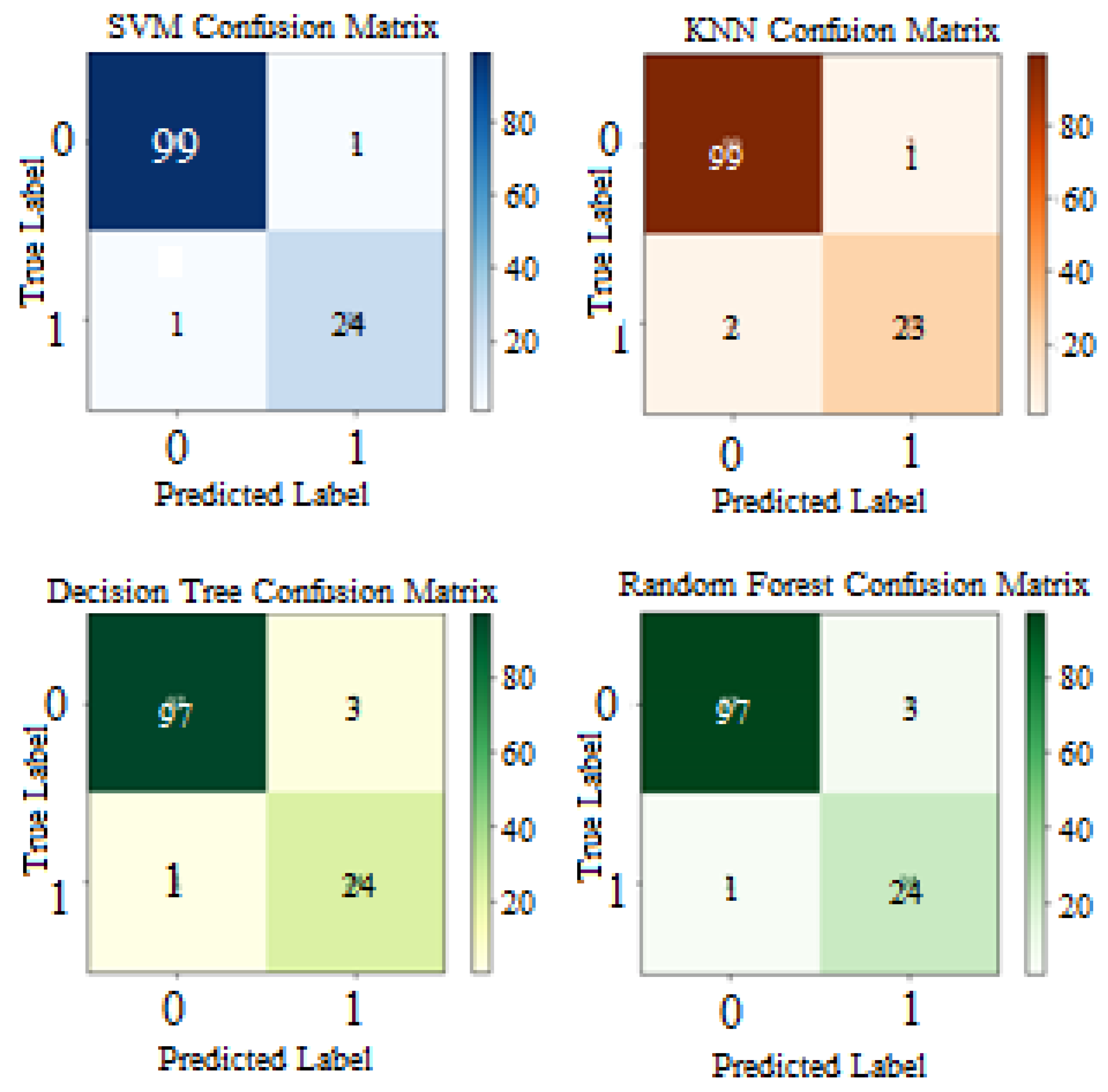
- True Positive (TP): the model predicted positive, and the actual value is positive (true). Real-world interpretation: there is a ‘seizure’ event in the EEG record, and the classifier accurately detected that EEG record as a ‘seizure’ case.
- True Negative (TN): the model predicted negative, and the actual value is negative (true). Real-world interpretation: there is no presence of ‘seizure’ in the EEG record (normal EEG record), and the classifier correctly detected that EEG record as a ‘non-seizure’ case.
- False Positive (FP): the model predicted positive, and the actual value is negative (false/Type 1 error). Real-world interpretation: there is no ‘seizure’ occurrence in EEG signal (normal EEG signal), but the classifier detects that signal as a ‘seizure’ case, thus the classifier detected inaccurately.
- False Negative (FN): the model predicted negative, and the actual value is positive (false/Type 2 error). Real-world interpretation: the classifier detects the EEG recording that has ‘seizure’ as a ‘normal’ case, thus the classifier detected incorrectly.
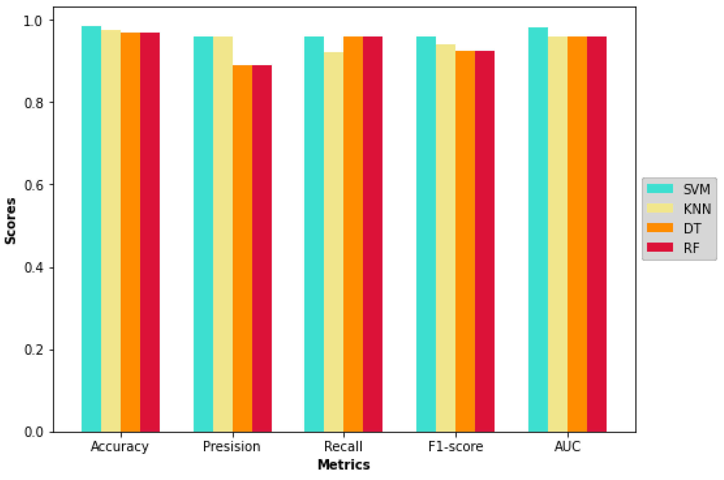
4.2. Proposed Model Results
4.3. Results Comparison
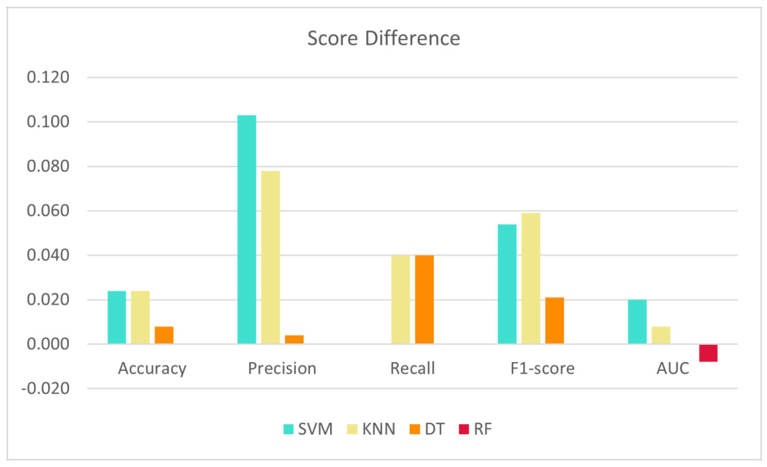
4.3.1. Compare with Baseline Results
4.3.2. Compare with Key Reference
4.4. Analysis
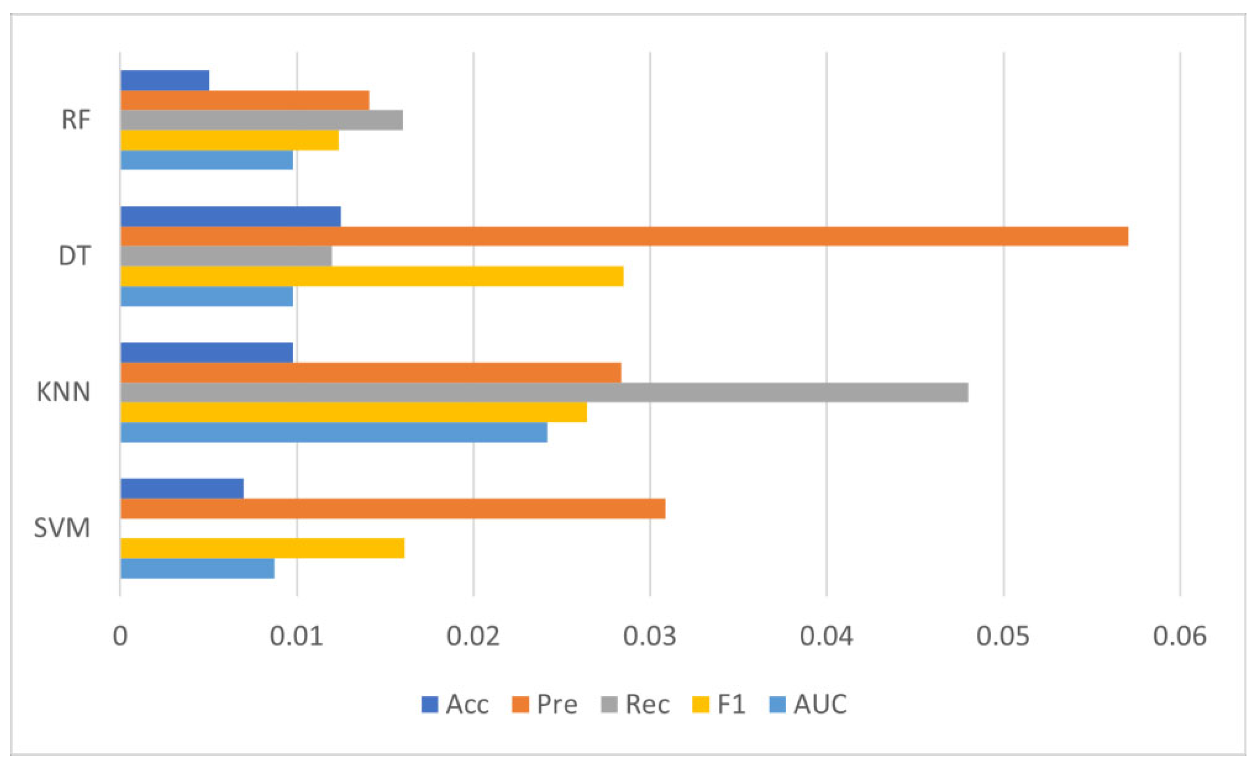
4.4.1. Model Validation
4.4.2. Sensitivity Analysis
Scenario 1: Iteration in FS-BPSO
Scenario 2: Initial Swarm and Considering Neighbors
4.5. Summary
5. Conclusions
- -
- Reproducibility: although the model has attained desirable results in the prototype, it struggles from deficient reproducibility when used in clinical practices. This is because ES prediction is a multiscale problem that is heavily influenced by the patient’s profile.
- -
- Generalization: another drawback is the lack of generalizability of this ES detection model among various seizure types and patients. Seizures often vary between patients who exhibit different features and biomarkers.
- -
- Seizure Heterogeneity: one of the factors that hinder the performance of the ES detection model is the heterogeneity of seizures. Consequently, there exists an imperative need for developing a ML model that is robust to the heterogeneity of epileptic seizure. This could be done by having a deeper understanding of seizure causes, seizure location, and how seizures spread.
- -
- The recommendations for future work on epileptic seizure detection are as follows:
- -
- Gain more insight into the detection of onset seizure events with real-time or near real-time monitoring of ES patients. This would enable doctors to provide timely treatment to patients before the onset of ES. Additionally, constant monitoring of ES patients using wearable EEG devices connected to smartphones and Internet of Things devices could significantly enhance the performance of machine learning models in predicting seizures.
- -
- Develop automatic data labeling methods, as seizure detection is usually devised as a classification task that requires labeled data. EEG recordings are manually labeled by neurologists, which is a costly and time-consuming task. Thus, it is imperative to optimize the data labeling process of EEG records.
Author Contributions
Funding
Institutional Review Board Statement
Informed Consent Statement
Data Availability Statement
Conflicts of Interest
References
- Sharma, M.; Pachori, R.B.; Acharya, U.R. A new approach to characterize epileptic seizures using analytic time-frequency flexible wavelet transform and fractal dimension. Pattern Recognit. Lett. 2017, 94, 172–179. [Google Scholar] [CrossRef]
- Pachori, R.B.; Patidar, S. Epileptic seizure classification in EEG signals using second-order difference plot of intrinsic mode functions. Comput. Methods Programs Biomed. 2014, 113, 494–502. [Google Scholar] [CrossRef]
- Rasheed, K.; Qayyum, A.; Qadir, J.; Sivathamboo, S.; Kwan, P.; Kuhlmann, L.; O’Brien, T.; Razi, A. Machine Learning for Predicting Epileptic Seizures Using EEG Signals: A Review. IEEE Rev. Biomed. Eng. 2021, 14, 139–155. [Google Scholar] [CrossRef] [PubMed]
- Zhou, M.; Tian, C.; Cao, R.; Wang, B.; Niu, Y.; Hu, T.; Guo, H.; Xiang, J. Epileptic Seizure Detection Based on EEG Signals and CNN. Front. Neuroinform. 2018, 12, 95. [Google Scholar] [CrossRef] [PubMed] [Green Version]
- Mula, M.; Monaco, F. Ictal and Peri-Ictal Psychopathology. Behav. Neurol. 2011, 24, 21–25. [Google Scholar] [CrossRef]
- Le, M.T.; Thanh Vo, M.; Mai, L.; Dao, S.V.T. Predicting heart failure using deep neural network. In Proceedings of the 2020 International Conference on Advanced Technologies for Communications (ATC), Nha Trang, Vietnam, 8–10 October 2020; pp. 221–225. [Google Scholar]
- Dao, S.V.T.; Yu, Z.; Tran, L.V.; Phan, P.N.K.; Huynh, T.T.M.; Le, T.M. An Analysis of Vocal Features for Parkinson’s Disease Classification Using Evolutionary Algorithms. Diagnostics 2022, 12, 1980. [Google Scholar] [CrossRef]
- Si, Y. Machine learning applications for electroencephalograph signals in epilepsy: A quick review. Acta Epileptol. 2020, 2, 8. [Google Scholar] [CrossRef]
- Ahammad, N.; Fathima, T.; Joseph, P. Detection of Epileptic Seizure Event and Onset Using EEG. BioMed Res. Int. 2014, 2014, 450573. [Google Scholar] [CrossRef]
- Siuly; Li, Y.; Wen, P. Clustering technique-based least square support vector machine for EEG signal classification. Comput. Methods Programs Biomed. 2011, 104, 358–372. [Google Scholar] [CrossRef]
- Savadkoohi, M.; Oladunni, T.; Thompson, L. A machine learning approach to epileptic seizure prediction using Electroencephalogram (EEG) Signal. Biocybern. Biomed. Eng. 2020, 40, 1328–1341. [Google Scholar] [CrossRef]
- Sharmila, A.; Geethanjali, P. DWT Based Detection of Epileptic Seizure From EEG Signals Using Naive Bayes and k-NN Classifiers. IEEE Access 2016, 4, 7716–7727. [Google Scholar] [CrossRef]
- Subasi, A.; Kevric, J.; Canbaz, M.A. Epileptic seizure detection using hybrid machine learning methods. Neural Comput. Appl. 2017, 31, 317–325. [Google Scholar] [CrossRef]
- Subasi, A.; Gursoy, M.I. EEG signal classification using PCA, ICA, LDA and support vector machines. Expert Syst. Appl. 2010, 37, 8659–8666. [Google Scholar] [CrossRef]
- Guo, L.; Rivero, D.; Dorado, J.; Rabuñal, J.R.; Pazos, A. Automatic epileptic seizure detection in EEGs based on line length feature and artificial neural73 networks. J. Neurosci. Methods 2010, 191, 101–109. [Google Scholar] [CrossRef] [PubMed]
- Tzallas, A.T.; Tsipouras, M.G.; Fotiadis, D.I. Automatic Seizure Detection Based on Time-Frequency Analysis and Artificial Neural Networks. Comput. Intell. Neurosci. 2007, 2007, 080510. [Google Scholar] [CrossRef] [PubMed]
- Mursalin; Zhang, Y.; Chen, Y.; Chawla, N.V. Automated epileptic seizure detection using improved correlation-based feature selection with random forest classifier. Neurocomputing 2017, 241, 204–214. [Google Scholar] [CrossRef]
- Sharma, R.R.; Varshney, P.; Pachori, R.B.; Vishvakarma, S.K. Automated System for Epileptic EEG Detection Using Iterative Filtering. IEEE Sens. Lett. 2018, 2, 1–4. [Google Scholar] [CrossRef]
- Wang, X.; Gong, G.; Li, N.; Qiu, S. Detection Analysis of Epileptic EEG Using a Novel Random Forest Model Combined With Grid Search Optimization. Front. Hum. Neurosci. 2019, 13, 52. [Google Scholar] [CrossRef] [Green Version]
- Yan, K.; Zhang, D. Feature selection and analysis on correlated gas sensor data with recursive feature elimination. Sens. Actuators B Chem. 2015, 212, 353–363. [Google Scholar] [CrossRef]
- Le, T.M.; Van Tran, L.; Dao, S.V.T. A Feature Selection Approach for Fall Detection Using Various Machine Learning Classifiers. IEEE Access 2021, 9, 115895–115908. [Google Scholar] [CrossRef]
- Le, M.T.; Vo, M.T.; Pham, N.T.; Dao, S.V. Predicting heart failure using a wrapper-based feature selection. Indones. J. Electr. Eng. Comput. Sci. 2021, 21, 1530–1539. [Google Scholar]
- El Aboudi, N.; Benhlima, L. Review on wrapper feature selection approaches. In Proceedings of the 2016 International Conference on Engineering & MIS (ICEMIS), Agadir, Morocco, 22–24 September 2016; pp. 1–5. [Google Scholar] [CrossRef]
- Le, T.M.; Pham, T.N.; Dao, S.V.T. A Novel Wrapper-Based Feature Selection for Heart Failure Prediction Using an Adaptive Particle Swarm Grey Wolf Optimization. In Enhanced Telemedicine and e-Health: Advanced IoT Enabled Soft Computing Framework; Marques, G., Bhoi, A.K., Díez, I.D., Garcia-Zapirain, B., Eds.; Springer International Publishing: Cham, Switzerland, 2021; pp. 315–336. [Google Scholar] [CrossRef]
- Pham, T.N.; Van Tran, L.; Dao, S.V.T. A Multi-Restart Dynamic Harris Hawk Optimization Algorithm for the Economic Load Dispatch Problem. IEEE Access 2021, 9, 122180–122206. [Google Scholar] [CrossRef]
- Liu, H.; Yu, L. Toward Integrating Feature Selection Algorithms for Classification and Clustering. IEEE Trans. Knowl. Data Eng. 2005, 17, 491–502. [Google Scholar]
- Chandrashekar, G.; Sahin, F. A survey on feature selection methods. Comput. Electr. Eng. 2014, 40, 16–28. [Google Scholar] [CrossRef]
- Tang, J.; Alelyani, S.; Liu, H. Feature Selection for Classification: A Review. Data Classif. Algorithms Appl. 2014, 37, 33. [Google Scholar]
- Tan, F. Improving Feature Selection Techniques for Machine Learning. Ph.D. Thesis, Georgia State University, Atlanta, GA, USA, 2007; p. 111. [Google Scholar]
- Jovic, A.; Brkic, K.; Bogunovic, N. A review of feature selection methods with applications. In Proceedings of the 2015 38th International Convention on Information and Communication Technology, Electronics and Microelectronics (MIPRO), Opatija, Croatia, 25–29 May 2015; pp. 1200–1205. [Google Scholar] [CrossRef]
- Yang, L.; Shami, A. On hyperparameter optimization of machine learning algorithms: Theory and practice. Neurocomputing 2020, 415, 295–316. [Google Scholar] [CrossRef]
- Hutter, F.; Kotthoff, L.; Vanschoren, J. (Eds.) Automated Machine Learning: Methods, Systems, Challenges; Springer International Publishing: Cham, Switzerland, 2019. [Google Scholar] [CrossRef] [Green Version]
- Yu, T.; Zhu, H. Hyper-Parameter Optimization: A Review of Algorithms and Applications. arXiv 2020, arXiv:2003.05689. [Google Scholar]
- Bergstra, J.; Bengio, Y. Random Search for Hyper-Parameter Optimization. J. Mach. Learn. Res. 2012, 13, 25. [Google Scholar]
- Sekeroglu, B.; Hasan, S.S.; Abdullah, S.M. Comparison of Machine Learning Algorithms for Classification Problems. In Advances in Computer Vision; Arai, K., Kapoor, S., Eds.; Springer International Publishing: Cham, Switzerland, 2020; Volume 944, pp. 491–499. [Google Scholar] [CrossRef]
- García-Gonzalo, E.; Fernández-Muñiz, Z.; Nieto, P.J.G.; Sánchez, A.B.; Fernández, M.M. Hard-Rock Stability Analysis for Span Design in Entry-Type Excavations with Learning Classifiers. Materials 2016, 9, 531. [Google Scholar] [CrossRef] [Green Version]
- Kotsiantis, S.B. Supervised Machine Learning: A Review of Classification Techniques. Emerg. Artif. Intell. Appl. Comput. Eng. 2007, 160, 3–24. [Google Scholar]
- Lan, T.; Hu, H.; Jiang, C.; Yang, G.; Zhao, Z. A comparative study of decision tree, random forest, and convolutional neural network for spread-F identification. Adv. Space Res. 2020, 65, 2052–2061. [Google Scholar] [CrossRef]
- Ali, J.; Khan, R.; Ahmad, N.; Maqsood, I. Random Forests and Decision Trees. Int. J. Comput. Sci. Issues (IJCSI) 2012, 9, 7. [Google Scholar]
- Dimitriadis, S.; Liparas, D.; Dni, A. How random is the random forest? Random forest algorithm on the service of structural imaging biomarkers for Alzheimer’s disease: From Alzheimer’s disease neuroimaging initiative (ADNI) database. Neural Regen. Res. 2018, 13, 962–970. [Google Scholar] [CrossRef]
- Wolpert, D.H. The Lack of A Priori Distinctions Between Learning Algorithms. Neural Comput. 1996, 8, 1341–1390. [Google Scholar] [CrossRef]
- Andrzejak, R.G.; Lehnertz, K.; Mormann, F.; Rieke, C.; David, P.; Elger, C.E. Indications of nonlinear deterministic and finite-dimensional structures in time series of brain electrical activity: Dependence on recording region and brain state. Phys. Rev. E 2001, 64, 061907. [Google Scholar] [CrossRef] [Green Version]
- Kennedy, J.; Eberhart, R. Particle swarm optimization. In Proceedings of the ICNN’95—International Conference on Neural Networks, Perth, WA, Australia, 27 November–1 December 1995; Volume 4, pp. 1942–1948. [Google Scholar] [CrossRef]
- Mafarja, M.; Jarrar, R.; Ahmad, S.; Abusnaina, A.A. Feature selection using binary particle swarm optimization with time varying inertia weight strategies. In Proceedings of the 2nd International Conference on Future Networks and Distributed Systems, Amman, Jordan, 26–27 June 2018; pp. 1–9. [Google Scholar] [CrossRef]
- Kennedy, J.; Eberhart, R.C. A discrete binary version of the particle swarm algorithm. In Proceedings of the 1997 IEEE International Conference on Systems, Man, and Cybernetics. Computational Cybernetics and Simulation, Orlando, FL, USA, 12–15 October 1997; Volume 5, pp. 4104–4108. [Google Scholar] [CrossRef]
- Jahromi, A.H.; Taheri, M. A non-parametric mixture of Gaussian naive Bayes classifiers based on local independent features. In Proceedings of the 2017 Artificial Intelligence and Signal Processing Conference (AISP), Shiraz, Iran, 25–27 October 2017; pp. 209–212. [Google Scholar] [CrossRef]
- Emary, E.; Zawbaa, H.M.; Hassanien, A.E. Binary grey wolf optimization approaches for feature selection. Neurocomputing 2016, 172, 371–381. [Google Scholar] [CrossRef]
- Galar, M.; Fernandez, A.; Barrenechea, E.; Bustince, H.; Herrera, F. A Review on Ensembles for the Class Imbalance Problem: Bagging-, Boosting-, and HybridBased Approaches. IEEE Trans. Syst. Man Cybern. Part C Appl. Rev. 2012, 42, 463–484. [Google Scholar] [CrossRef]
- Vieira, S.M.; Mendonça, L.F.; Farinha, G.J.; Sousa, J.M. Modified binary PSO for feature selection using SVM applied to mortality prediction of septic patients. Appl. Soft Comput. 2013, 13, 3494–3504. [Google Scholar] [CrossRef]
- Mandrekar, J.N. Receiver Operating Characteristic Curve in Diagnostic Test Assessment. J. Thorac. Oncol. 2010, 5, 1315–1316. [Google Scholar] [CrossRef] [Green Version]
- Wang, L.; Xue, W.; Li, Y.; Luo, M.; Huang, J.; Cui, W.; Huang, C. Automatic Epileptic Seizure Detection in EEG Signals Using Multi-Domain Feature Extraction and Nonlinear Analysis. Entropy 2017, 19, 222. [Google Scholar] [CrossRef] [Green Version]
- Kumar, Y.; Dewal, M.; Anand, R. Epileptic seizure detection using DWT based fuzzy approximate entropy and support vector machine. Neurocomputing 2014, 133, 271–279. [Google Scholar] [CrossRef]
- Jaiswal, A.K.; Banka, H. Epileptic seizure detection in EEG signal using machine learning techniques. Australas. Phys. Eng. Sci. Med. 2017, 41, 81–94. [Google Scholar] [CrossRef] [PubMed]


| Set | Symbol | Patients | Description | Segments |
|---|---|---|---|---|
| A | Z | Healthy | No seizure | 100 |
| B | O | Healthy | No seizure | 100 |
| C | N | Epilepsy | Inter-ictal (seizure-free) | 100 |
| D | F | Epilepsy | Inter-ictal (seizure-free) | 100 |
| E | S | Epilepsy | Seizure occurrence | 100 |
| Features | Coeff. A5 | Coeff. D3 | Coeff. D4 | Coeff. D5 |
|---|---|---|---|---|
| Minimum | f1 | f11 | f21 | f31 |
| Maximum | f2 | f12 | f22 | f32 |
| Median | f3 | f13 | f23 | f33 |
| Mean | f4 | f14 | f24 | f34 |
| Standard Deviation | f5 | f15 | f25 | f35 |
| Variance | f6 | f16 | f26 | f36 |
| Root Mean Square | f7 | f17 | f27 | f37 |
| Kurtosis | f8 | f18 | f28 | f38 |
| Skewness | f9 | f19 | f29 | f39 |
| No. of Zero Crossings | f10 | f20 | f30 | f40 |
| Features | SVM | KNN | DT | RF |
|---|---|---|---|---|
| Accuracy | 0.960 | 0.952 | 0.960 | 0.968 |
| Precision | 0.857 | 0.880 | 0.885 | 0.889 |
| Recall | 0.960 | 0.880 | 0.920 | 0.960 |
| F1-score | 0.906 | 0.880 | 0.902 | 0.923 |
| AUC | 0.960 | 0.952 | 0.960 | 0.968 |
| Computational time (s) | 1.644 | 1.266 | 1.297 | 1.978 |
| Features | Selected | Features | Selected | Features | Selected | Features | Selected |
|---|---|---|---|---|---|---|---|
| f1 | x | f11 | f21 | f31 | |||
| f2 | f12 | f22 | x | f32 | |||
| f3 | f13 | f23 | f33 | ||||
| f4 | x | f14 | f24 | f34 | |||
| f5 | f15 | f25 | x | f35 | |||
| f6 | f16 | f26 | x | f36 | |||
| f7 | x | f17 | f27 | f37 | |||
| f8 | f18 | x | f28 | f38 | |||
| f9 | f19 | f29 | f39 | x | |||
| f10 | f20 | f30 | x | f40 | x |
| Classifier | Hyperparameter Search Space |
|---|---|
| SVM | C; float number in range (0, 50) kernel: linear, polynomial, rbf, sigmoid |
| KNN | K: even numbers in range (3, 20) Weight: uniform, distance Distance: Euclidean, Manhattan, Chebyshev, Minkowski |
| DT | max_depth: integer numbers in range (3, 50) min_samples_leaf: integer numbers in range (3, 100) min_samples_split: integer numbers in range (2, 50) |
| RF | max_depth: integer numbers in range (5, 50) min_samples_leaf: integer numbers in range (2, 11) min_samples_split: integer numbers in range (2, 11) n_estimator: integer numbers in range (10, 100) criterion: gini, entropy |
| Predicted Negative (0) | Predicted Positive (1) | |
|---|---|---|
| Actual Negative (0) | True Negative (TN) | False Positive (FP) |
| Actual Positive (1) | False Negative (FN) | True Positive (TP) |
| Classifier | Predicted Negative (0) | Accuracy of the Training Set from RS |
|---|---|---|
| SVM | C: 17.9384479998486 | 99.2% |
| Kernel: rbf | ||
| KNN | K: 5 | 98.6% |
| weight: distance | ||
| distance: euclidean | ||
| DT | max_depth: 37 | 97.3% |
| min_samples_leaf: 3 | ||
| min_sample_split: 37 | ||
| RF | max_depth: 46 | 98.4% |
| min_samples_leaf: 2 | ||
| min_sample_split: 4 | ||
| n_estimator: 96 | ||
| criterion: entropy |
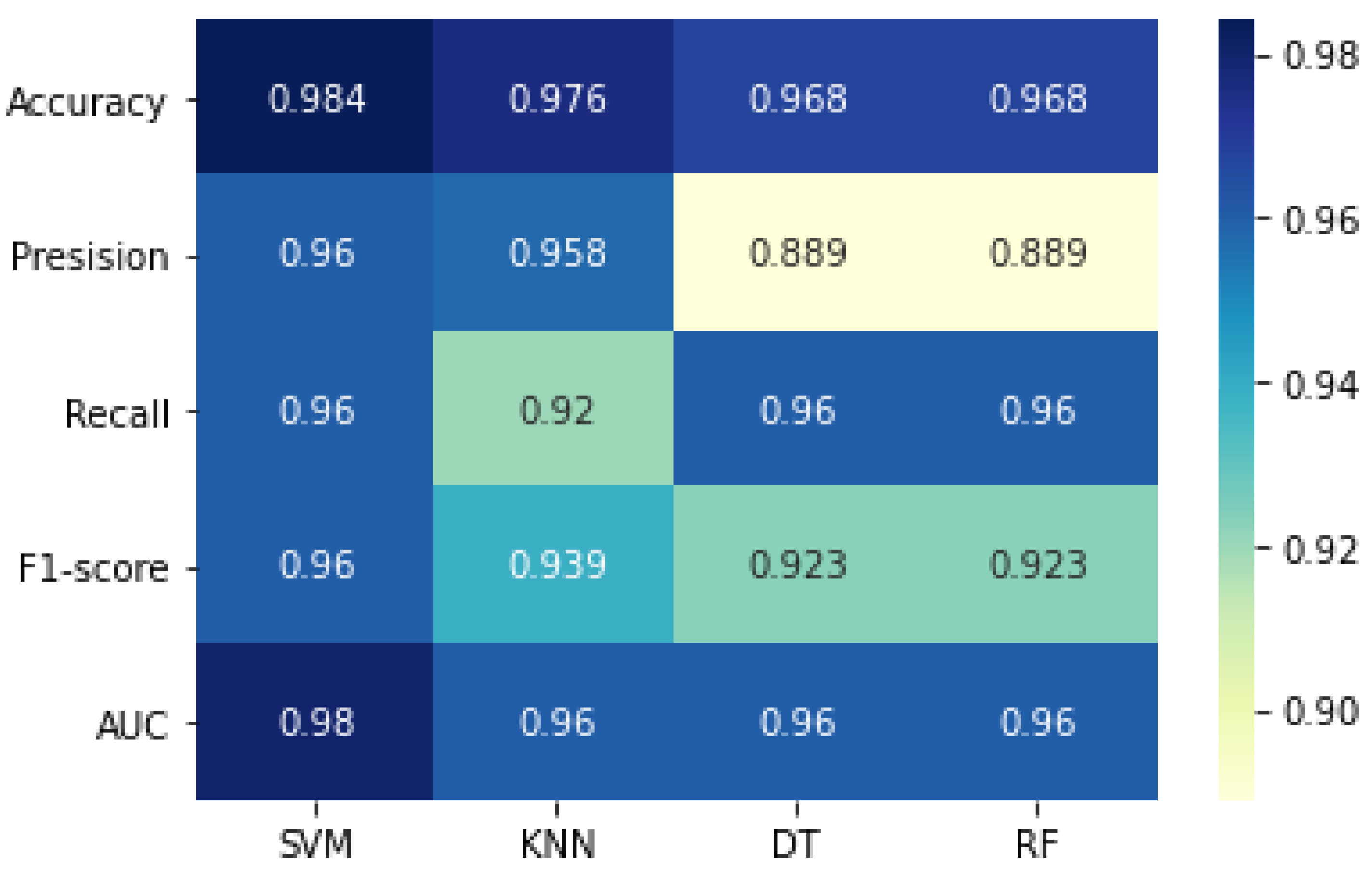
| SVM | KNN | DT | RF | |
|---|---|---|---|---|
| Accuracy | 0.984 | 0.976 | 0.968 | 0.968 |
| Precision | 0.960 | 0.958 | 0.889 | 0.889 |
| Recall | 0.960 | 0.920 | 0.960 | 0.960 |
| F1-score | 0.960 | 0.939 | 0.923 | 0.923 |
| AUC | 0.980 | 0.960 | 0.960 | 0.960 |
| Computational time (s) | 1.22 | 1.140 | 1.087 | 1.667 |
| SVM | KNN | DT | RF | |
|---|---|---|---|---|
| Accuracy | +2.4% | +2.5% | +0.8% | - |
| Precision | +10.7% | +8.1% | +0.4% | - |
| Recall | - | +4.3% | +4.2% | - |
| F1-score | +5.6% | +6.3% | +2.3% | - |
| AUC | +2.0% | +0.8% | - | −0.8% |
| Computational time (s) | −46.5% | −11.1% | −19.3% | −18.7% |
| SVM | KNN | DT | RF | |
|---|---|---|---|---|
| Baseline | 1.644 | 1.266 | 1.297 | 1.978 |
| Proposed Model | 1.122 | 1.140 | 1.087 | 1.667 |
| Percent reduced | −46.5% | −11.1% | −19.3% | −18.7% |
| SVM | KNN | DT | RF | Key Ref. | |
|---|---|---|---|---|---|
| Accuracy | 98.40% | 97.60% | 96.80% | 06.80% | 97.10% |
| Sensitivity | 96.00% | 92.00% | 96.00% | 96.00% | 93.62% |
| Specificity | 99.00% | 99.00% | 97.00% | 97.00% | 97.94% |
| Accuracy | Precision | Recall | F1-Score | AUC | |
|---|---|---|---|---|---|
| Trial 1 | 0.984 | 0.960 | 0.960 | 0.960 | 0.980 |
| Trial 2 | 0.968 | 0.889 | 0.960 | 0.923 | 0.960 |
| Trial 3 | 0.968 | 0.889 | 0.960 | 0.923 | 0.960 |
| Trial 4 | 0.968 | 0.889 | 0.960 | 0.923 | 0.960 |
| Trial 5 | 0.984 | 0.960 | 0.960 | 0.960 | 0.980 |
| Trial 6 | 0.984 | 0.960 | 0.960 | 0.960 | 0.980 |
| Trial 7 | 0.976 | 0.923 | 0.960 | 0.941 | 0.970 |
| Trial 8 | 0.968 | 0.889 | 0.960 | 0.923 | 0.960 |
| Trial 9 | 0.968 | 0.889 | 0.960 | 0.923 | 0.960 |
| Trial 10 | 0.976 | 0.923 | 0.960 | 0.941 | 0.970 |
| Mean | 0.974 | 0.917 | 0.96 | 0.938 | 0.968 |
| Std | 0.007 | 0.031 | 0.000 | 0.016 | 0.009 |
| Accuracy | Precision | Recall | F1-Score | AUC | |
|---|---|---|---|---|---|
| Trial 1 | 0.976 | 0.958 | 0.920 | 0.939 | 0.960 |
| Trial 2 | 0.952 | 0.952 | 0.800 | 0.870 | 0.900 |
| Trial 3 | 0.976 | 0.958 | 0.920 | 0.939 | 0.960 |
| Trial 4 | 0.968 | 0.920 | 0.920 | 0.920 | 0.950 |
| Trial 5 | 0.984 | 0.960 | 0.960 | 0.960 | 0.980 |
| Trial 6 | 0.960 | 0.955 | 0.840 | 0.894 | 0.910 |
| Trial 7 | 0.952 | 0.880 | 0.880 | 0.880 | 0.920 |
| Trial 8 | 0.968 | 0.920 | 0.920 | 0.920 | 0.950 |
| Trial 9 | 0.968 | 0.889 | 0.960 | 0.923 | 0.960 |
| Trial 10 | 0.968 | 0.920 | 0.920 | 0.920 | 0.950 |
| Mean | 0.967 | 0.931 | 0.90 | 0.917 | 0.944 |
| Std | 0.010 | 0.028 | 0.048 | 0.026 | 0.024 |
| Accuracy | Precision | Recall | F1-Score | AUC | |
|---|---|---|---|---|---|
| Trial 1 | 0.968 | 0.889 | 0.960 | 0.923 | 0.960 |
| Trial 2 | 0.984 | 1.000 | 0.920 | 0.958 | 0.960 |
| Trial 3 | 0.952 | 0.852 | 0.920 | 0.885 | 0.940 |
| Trial 4 | 0.976 | 0.958 | 0.920 | 0.939 | 0.960 |
| Trial 5 | 0.984 | 1.000 | 0.920 | 0.958 | 0.960 |
| Trial 6 | 0.960 | 0.885 | 0.920 | 0.902 | 0.940 |
| Trial 7 | 0.944 | 0.821 | 0.920 | 0.868 | 0.940 |
| Trial 8 | 0.960 | 0.885 | 0.920 | 0.902 | 0.940 |
| Trial 9 | 0.960 | 0.885 | 0.920 | 0.902 | 0.940 |
| Trial 10 | 0.960 | 0.885 | 0.920 | 0.902 | 0.940 |
| Mean | 0.965 | 0.906 | 0.924 | 0.914 | 0.948 |
| Std | 0.012 | 0.057 | 0.012 | 0.028 | 0.010 |
| Accuracy | Precision | Recall | F1-Score | AUC | |
|---|---|---|---|---|---|
| Trial 1 | 0.968 | 0.889 | 0.960 | 0.923 | 0.960 |
| Trial 2 | 0.968 | 0.889 | 0.960 | 0.923 | 0.960 |
| Trial 3 | 0.960 | 0.885 | 0.920 | 0.902 | 0.940 |
| Trial 4 | 0.968 | 0.889 | 0.960 | 0.923 | 0.960 |
| Trial 5 | 0.976 | 0.923 | 0.960 | 0.941 | 0.970 |
| Trial 6 | 0.976 | 0.923 | 0.960 | 0.941 | 0.970 |
| Trial 7 | 0.968 | 0.889 | 0.960 | 0.923 | 0.960 |
| Trial 8 | 0.960 | 0.885 | 0.920 | 0.902 | 0.940 |
| Trial 9 | 0.968 | 0.889 | 0.960 | 0.923 | 0.960 |
| Trial 10 | 0.968 | 0.889 | 0.960 | 0.923 | 0.960 |
| Mean | 0.968 | 0.895 | 0.952 | 0.922 | 0.958 |
| Std | 0.005 | 0.014 | 0.016 | 0.012 | 0.010 |
| Classifier | Iteration | Accuracy | Precision | Recall | F1-Score | AUC |
|---|---|---|---|---|---|---|
| SVM | 50 | 0.96 | 0.85 | 0.92 | 0.902 | 0.94 |
| 100 | 0.96 | 0.885 | 0.92 | 0.902 | 0.94 | |
| 500 | 0.968 | 0.889 | 0.96 | 0.923 | 0.96 | |
| 1000 | 0.984 | 0.96 | 0.96 | 0.96 | 0.98 | |
| 3000 | 0.976 | 0.923 | 0.96 | 0.941 | 0.97 | |
| 5000 | 0.952 | 0.88 | 0.88 | 0.88 | 0.92 | |
| KNN | 50 | 0.96 | 0.917 | 0.88 | 0.898 | 0.93 |
| 100 | 0.968 | 0.92 | 0.92 | 0.92 | 0.95 | |
| 500 | 0.968 | 0.92 | 0.92 | 0.92 | 0.95 | |
| 1000 | 0.976 | 0.958 | 0.92 | 0.939 | 0.96 | |
| 3000 | 0.968 | 0.92 | 0.92 | 0.92 | 0.95 | |
| 5000 | 0.96 | 0.917 | 0.88 | 0.898 | 0.93 | |
| DT | 50 | 0.984 | 1 | 0.92 | 0.958 | 0.96 |
| 100 | 0.96 | 0.885 | 0.92 | 0.902 | 0.94 | |
| 500 | 0.976 | 0.958 | 0.92 | 0.939 | 0.96 | |
| 1000 | 0.968 | 0.889 | 0.96 | 0.923 | 0.96 | |
| 3000 | 0.96 | 0.885 | 0.92 | 0.902 | 0.94 | |
| 5000 | 0.968 | 0.92 | 0.92 | 0.92 | 0.95 | |
| RF | 50 | 0.968 | 0.92 | 0.92 | 0.92 | 0.95 |
| 100 | 0.968 | 0.885 | 0.92 | 0.902 | 0.94 | |
| 500 | 0.968 | 0.889 | 0.96 | 0.923 | 0.96 | |
| 1000 | 0.968 | 0.889 | 0.96 | 0.923 | 0.96 | |
| 3000 | 0.968 | 0.885 | 0.92 | 0.902 | 0.94 | |
| 5000 | 0.96 | 0.885 | 0.92 | 0.902 | 0.94 |
| Classifier | Iteration | Accuracy | Precision | Recall | F1-Score | AUC |
|---|---|---|---|---|---|---|
| SVM | 10 | 0.968 | 0.889 | 0.96 | 0.923 | 0.96 |
| 20 | 0.968 | 0.889 | 0.96 | 0.923 | 0.96 | |
| 30 | 0.976 | 0.923 | 0.96 | 0.941 | 0.97 | |
| 40 | 0.984 | 0.96 | 0.96 | 0.96 | 0.98 | |
| 60 | 0.968 | 0.889 | 0.96 | 0.923 | 0.96 | |
| 80 | 0.976 | 0.923 | 0.96 | 0.941 | 0.97 | |
| 80 | 0.976 | 0.923 | 0.96 | 0.941 | 0.97 | |
| KNN | 10 | 0.96 | 0.917 | 0.88 | 0.898 | 0.93 |
| 20 | 0.976 | 0.958 | 0.92 | 0.939 | 0.96 | |
| 30 | 0.976 | 0.923 | 0.96 | 0.941 | 0.97 | |
| 40 | 0.976 | 0.958 | 0.92 | 0.939 | 0.96 | |
| 60 | 0.944 | 0.875 | 0.84 | 0.857 | 0.9 | |
| 60 | 0.944 | 0.875 | 0.84 | 0.857 | 0.9 | |
| 60 | 0.944 | 0.875 | 0.84 | 0.857 | 0.9 | |
| DT | 10 | 0.952 | 0.852 | 0.92 | 0.885 | 0.94 |
| 20 | 0.96 | 0.885 | 0.92 | 0.902 | 0.94 | |
| 30 | 0.96 | 0.885 | 0.92 | 0.902 | 0.94 | |
| 40 | 0.968 | 0.889 | 0.96 | 0.923 | 0.96 | |
| 60 | 0.976 | 0.958 | 0.92 | 0.939 | 0.96 | |
| 80 | 0.976 | 0.923 | 0.96 | 0.941 | 0.97 | |
| 100 | 0.968 | 0.862 | 1 | 0.926 | 0.98 | |
| RF | 10 | 0.96 | 0.885 | 0.92 | 0.902 | 0.94 |
| 20 | 0.976 | 0.923 | 0.96 | 0.941 | 0.97 | |
| 30 | 0.968 | 0.889 | 0.96 | 0.923 | 0.96 | |
| 40 | 0.968 | 0.889 | 0.96 | 0.923 | 0.96 | |
| 60 | 0.96 | 0.885 | 0.92 | 0.902 | 0.94 | |
| 80 | 0.968 | 0.889 | 0.96 | 0.923 | 0.96 | |
| 100 | 0.968 | 0.889 | 0.96 | 0.923 | 0.96 |
Publisher’s Note: MDPI stays neutral with regard to jurisdictional claims in published maps and institutional affiliations. |
© 2022 by the authors. Licensee MDPI, Basel, Switzerland. This article is an open access article distributed under the terms and conditions of the Creative Commons Attribution (CC BY) license (https://creativecommons.org/licenses/by/4.0/).
Share and Cite
Tran, L.V.; Tran, H.M.; Le, T.M.; Huynh, T.T.M.; Tran, H.T.; Dao, S.V.T. Application of Machine Learning in Epileptic Seizure Detection. Diagnostics 2022, 12, 2879. https://doi.org/10.3390/diagnostics12112879
Tran LV, Tran HM, Le TM, Huynh TTM, Tran HT, Dao SVT. Application of Machine Learning in Epileptic Seizure Detection. Diagnostics. 2022; 12(11):2879. https://doi.org/10.3390/diagnostics12112879
Chicago/Turabian StyleTran, Ly V., Hieu M. Tran, Tuan M. Le, Tri T. M. Huynh, Hung T. Tran, and Son V. T. Dao. 2022. "Application of Machine Learning in Epileptic Seizure Detection" Diagnostics 12, no. 11: 2879. https://doi.org/10.3390/diagnostics12112879