Deep Learning-Based Morphological Classification of Human Sperm Heads


Abstract
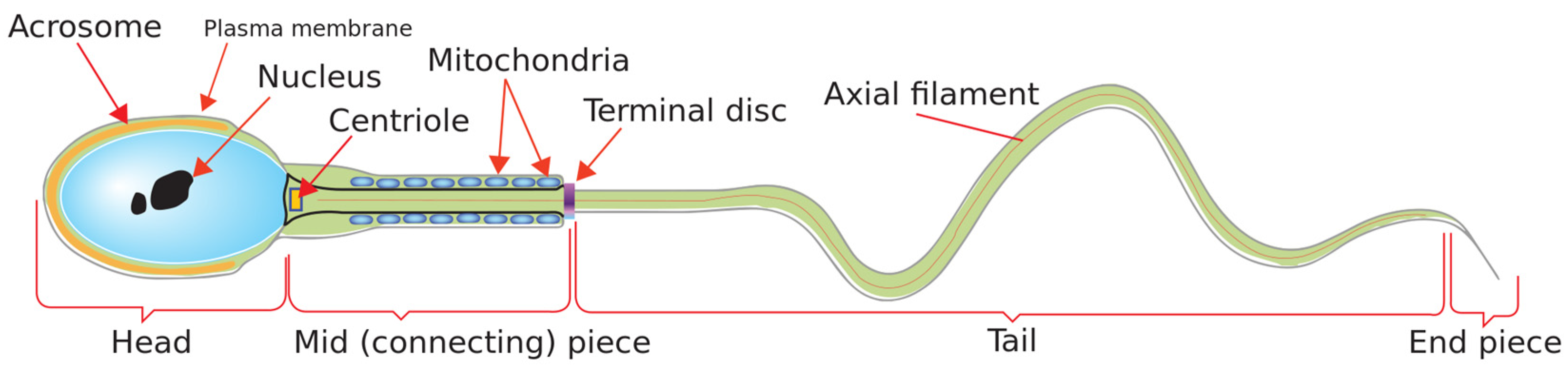
:1. Introduction
2. Related Work
3. Methodology
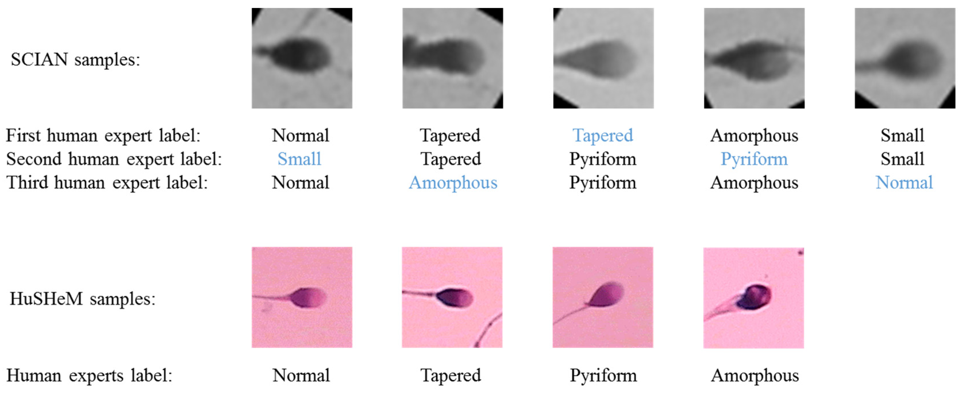
3.1. Datasets Descrption, Partitioning, and Augmentation
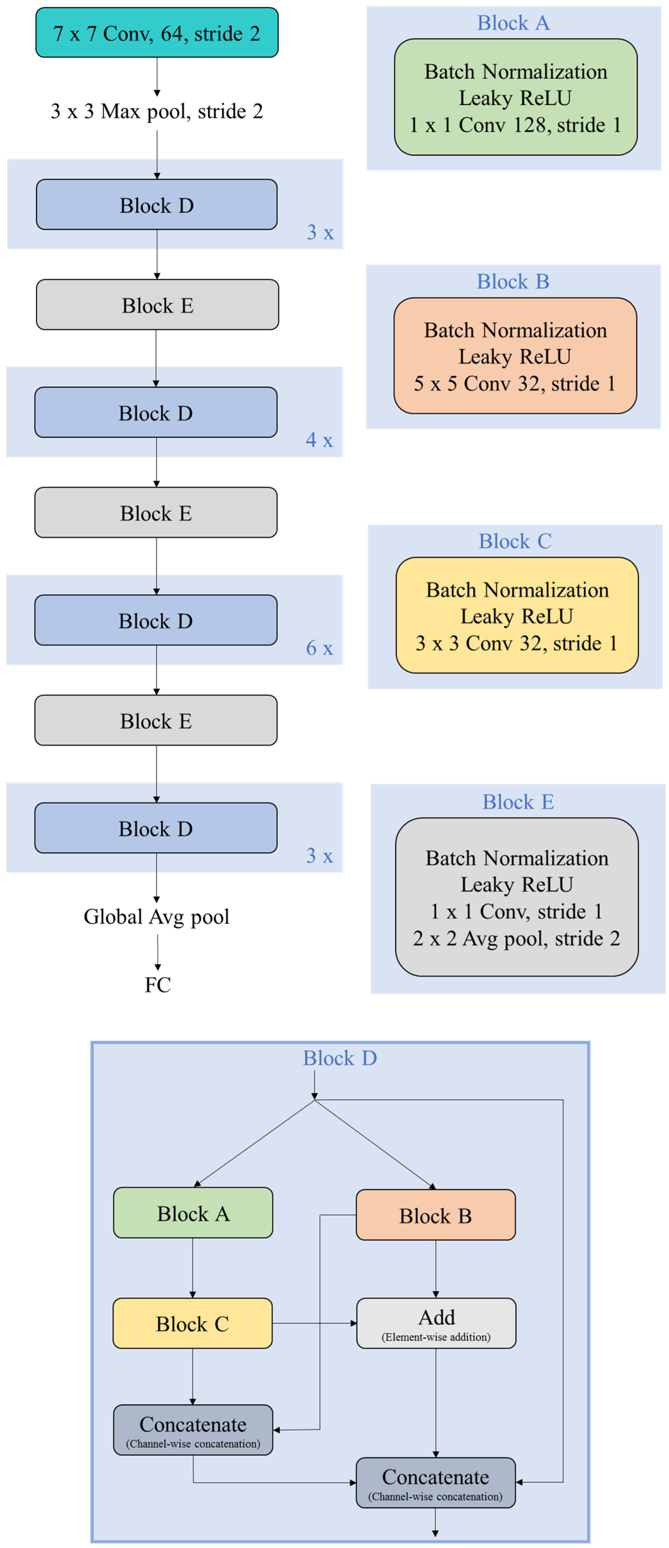
3.2. Proposed Deep CNN Architecture and Learning Paradigm
4. Experimental Results
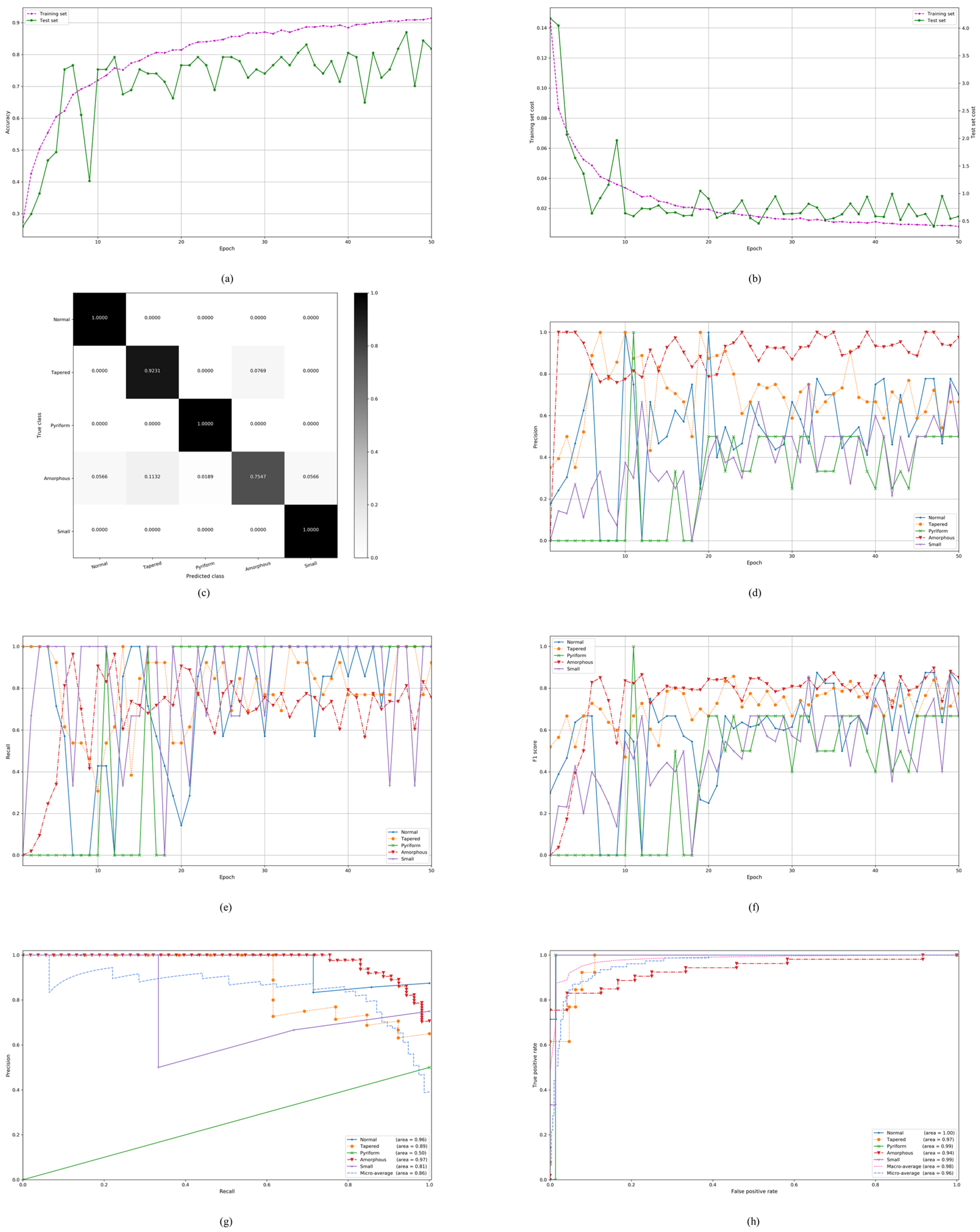
4.1. On the Stratified Five-Fold Partition of the SCIAN Dataset with the Partial Agreement Setting
4.2. On the Stratified Five-Fold Partition of the SCIAN Dataset with the Total Agreement Setting
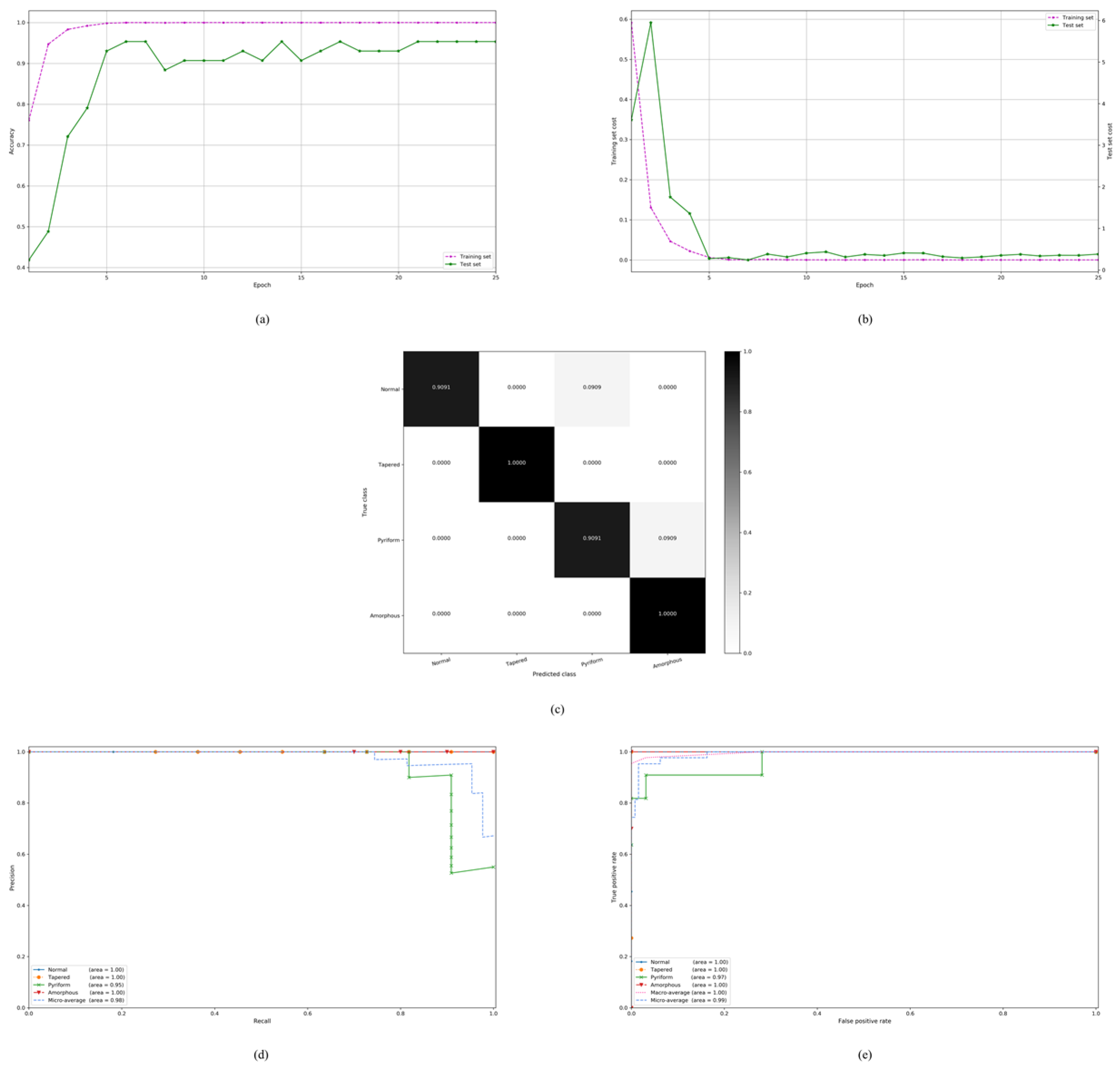
4.3. On the Stratified Five-Fold Partition of the HuSHeM Dataset
5. Discussion and Conclusions
Supplementary Materials
Author Contributions
Funding
Acknowledgments
Conflicts of Interest
References
- Villarreal, M.R. Complete Diagram of a Human Spermatozoon. Available online: https://commons.wikimedia.org/wiki/File:Complete_diagram_of_a_human_spermatozoa_en.svg (accessed on 9 October 2019).
- Zegers-Hochschild, F.; Adamson, G.D.; De Mouzon, J.; Ishihara, O.; Mansour, R.; Nygren, K.; Sullivan, E.; Vanderpoel, S. International Committee for Monitoring Assisted Reproductive Technology (ICMART) and the World Health Organization (WHO) revised glossary of ART. Fertil. Steril. 2009, 92, 1520–1524. [Google Scholar] [CrossRef] [PubMed]
- Blasco, V.; Pinto, F.M.; Gonz, C.; Santamar, E.; Candenas, L.; Fern, M. Tachykinins and Kisspeptins in the Regulation of Human Male Fertility. J. Clin. Med. 2020, 9, 113. [Google Scholar] [CrossRef] [PubMed] [Green Version]
- Wang, S.-C.; Wang, S.-C.; Li, C.-J.; Lin, C.-H.; Huang, H.-L.; Tsai, L.-M.; Chang, C.-H. The Therapeutic Effects of Traditional Chinese Medicine for Poor Semen Quality in Infertile Males. J. Clin. Med. 2018, 7, 239. [Google Scholar] [CrossRef] [PubMed] [Green Version]
- Kidd, S.A.; Eskenazi, B.; Wyrobek, A.J. Effects of male age on semen quality and fertility: A review of the literature. Fertil. Steril. 2001, 75, 237–248. [Google Scholar] [CrossRef]
- Barone, M.A.; Roelke, M.E.; Howard, J.; Brown, J.L.; Anderson, A.E.; Wildt, D.E. Reproductive Characteristics of Male Florida Panthers: Comparative studies from Florida, Texas, Colorado, Latin America, and North American Zoos. J. Mammal. 1994, 75, 150–162. [Google Scholar] [CrossRef] [Green Version]
- Monte, G.L.; Murisier, F.; Piva, I.; Germond, M.; Marci, R. Focus on intracytoplasmic morphologically selected sperm injection ( IMSI ): A mini-review. Asian J. Androl. 2013, 15, 608–615. [Google Scholar] [CrossRef] [Green Version]
- Maduro, M.R.; Lamb, D.J. Understanding the new genetics of male infertility. J. Urol. 2002. [Google Scholar]
- World Health Organization. WHO Laboratory Manual for the Examination and Processing of Human Semen, 5th ed.; World Health Organization: Geneva, Switzerland, 2010. [Google Scholar]
- Brazil, C. Practical semen analysis: From A to Z. Asian J. Androl. 2010, 12, 14–20. [Google Scholar] [CrossRef] [Green Version]
- Gatimel, N.; Moreau, J.; Parinaud, J.; Léandri, R.D. Sperm morphology: Assessment, pathophysiology, clinical relevance, and state of the art in 2017. Andrology 2017, 5, 845–862. [Google Scholar] [CrossRef] [Green Version]
- Mortimer, S.T.; Van Der Horst, G.; Mortimer, D. The future of computer-aided sperm analysis. Asian J. Androl. 2015, 17, 545–553. [Google Scholar] [CrossRef]
- Menkveld, R.; Holleboom, C.A.G.; Rhemrev, J.P.T. Measurement and significance of sperm morphology. Asian J. Androl. 2011, 13, 59–68. [Google Scholar] [CrossRef] [PubMed] [Green Version]
- Chang, V.; Garcia, A.; Hitschfeld, N.; Hartel, S. Gold-standard for computer-assisted morphological sperm analysis. Comput. Biol. Med. 2017, 83, 143–150. [Google Scholar] [CrossRef] [PubMed]
- Yi, W.J.; Park, K.S.; Paick, J.S. Parameterized characterization of elliptic sperm heads using Fourier representation and wavelet transform. In Proceedings of the Annual International Conference of the ZEEE Engineering in Medicine and Biology Society, Hong Kong, China, 1 November 1998; Volume 20, pp. 974–977. [Google Scholar]
- Li, J.; Tseng, K.K.; Dong, H.; Li, Y.; Zhao, M.; Ding, M. Human sperm health diagnosis with principal component analysis and k-nearest neighbor algorithm. In Proceedings of the International Conference on Medical Biometrics, Shenzhen, China, 30 May–1 June 2014; IEEE: Shenzhen, China, 2014; pp. 108–113. [Google Scholar]
- Beletti, M.E.; Costa, L.D.F.; Viana, M.P. A comparison of morphometric characteristics of sperm from fertile Bos taurus and Bos indicus bulls in Brazil. Anim. Reprod. Sci. 2005, 85, 105–116. [Google Scholar] [CrossRef] [PubMed]
- Severa, L.; Máchal, L.; Švábová, L.; Mamica, O. Evaluation of shape variability of stallion sperm heads by means of image analysis and Fourier descriptors. Anim. Reprod. Sci. 2010, 119, 50–55. [Google Scholar] [CrossRef]
- Chang, V.; Heutte, L.; Petitjean, C.; Hartel, S.; Hitschfeld, N. Automatic classification of human sperm head morphology. Comput. Biol. Med. 2017, 84, 205–216. [Google Scholar] [CrossRef]
- Shaker, F.; Monadjemi, S.A.; Alirezaie, J.; Naghsh-Nilchi, A.R. A dictionary learning approach for human sperm heads classification. Comput. Biol. Med. 2017, 91, 181–190. [Google Scholar] [CrossRef]
- Riordon, J.; Mccallum, C.; Sinton, D. Deep learning for the classification of human sperm. Comput. Biol. Med. 2019, 111. [Google Scholar] [CrossRef]
- Russakovsky, O.; Deng, J.; Su, H.; Krause, J.; Satheesh, S.; Ma, S.; Huang, Z.; Karpathy, A.; Jan, C.V.; Krause, J.; et al. ImageNet Large Scale Visual Recognition Challenge. Int. J. Comput. Vis. 2015, 115, 211–252. [Google Scholar] [CrossRef] [Green Version]
- Szegedy, C.; Liu2, W.; Jia, Y.; Sermanet, P.; Reed, S.; Anguelov, D.; Erhan1, D.; Vanhoucke, V.; Rabinovich, A. Going Deeper with Convolutions. In Proceedings of the IEEE Conference on Computer Vision and Pattern Recognition (CVPR), Boston, MA, USA, 7–12 June 2015. [Google Scholar]
- Ronneberger, O.; Fischer, P.; Brox, T. U-net: Convolutional networks for biomedical image segmentation. In Proceedings of the International Conference on Medical Image Computing and Computer-Assisted Intervention, Munich, Germany, 5–9 October 2015; Volume 9351, pp. 234–241. [Google Scholar]
- He, K.; Zhang, X.; Ren, S.; Sun, J. Deep Residual Learning for Image Recognition. In Proceedings of the Computer Vision and Pattern Recognition, Las Vegas, NV, USA, 26 June–1 July 2016; pp. 770–778. [Google Scholar]
- Chollet, F. Xception: Deep learning with depthwise separable convolutions. In Proceedings of the Conference on Computer Vision and Pattern Recognition, Honolulu, HI, USA, 21–26 July 2017; pp. 1800–1807. [Google Scholar]
- Huang, G.; Liu, Z.; Van Der Maaten, L.; Weinberger, K.Q. Densely connected convolutional networks. In Proceedings of the Conference on Computer Vision and Pattern Recognition, Honolulu, HI, USA, 21–26 July 2017; pp. 2261–2269. [Google Scholar]
- Iqbal, I.; Shahzad, G.; Rafiq, N.; Mustafa, G.; Ma, J. Deep learning-based automated detection of human knee joint’s synovial fluid from magnetic resonance images with transfer learning. IET Image Process. 2020. (In press) [Google Scholar]
- Ioffe, S.; Szegedy, C. Batch Normalization: Accelerating Deep Network Training by Reducing Internal Covariate Shift. arXiv 2015, arXiv:1502.03167. [Google Scholar]
- Maas, A.L.; Hannun, A.Y.; Ng, A.Y. Rectifier Nonlinearities Improve Neural Network Acoustic Models. In Proceedings of the International Conference on Machine Learning, Atlanta, GA, USA, 16 June–21 June 2013; Volume 28. [Google Scholar]
- LeCun, Y.A.; Bottou, L.; Orr, G.B.; Müller, K.-R. Efficient BackProp; Springer: Heidelberg, Germany, 2012. [Google Scholar]
- Kingma, D.P.; Ba, J.L. Adam: A Method for Stochastic Optimization. In Proceedings of the 3rd International Conference on Learning Representations, San Diego, CA, USA, 7–9 May 2015. [Google Scholar]
- Chollet, F. Keras (2015). Available online: http//keras.io (accessed on 9 October 2019).
- Abadi, M.; Agarwal, A.; Barham, P.; Brevdo, E.; Chen, Z.; Citro, C.; Corrado, G.S.; Davis, A.; Dean, J.; Devin, M.; et al. TensorFlow: Large-Scale Machine Learning on Heterogeneous Distributed Systems. arXiv 2016, arXiv:1603.04467. [Google Scholar]


| Fold | Set | Sperm Head Classes | Total | ||||
|---|---|---|---|---|---|---|---|
| Normal | Tapered | Pyriform | Amorphous | Small | |||
| 1 | Train | 80–20 (4860) | 182–46 (4896) | 60–15 (4860) | 525–131 (4728) | 58–14 (4840) | 905–226 (24184) |
| Test | 20 | 46 | 16 | 131 | 14 | 227 | |
| 2 and 3 | Train | 80 (6400) | 182 (6370) | 61 (6405) | 525 (6300) | 58 (6380) | 906 (31855) |
| Test | 20 | 46 | 15 | 131 | 14 | 226 | |
| 4 | Train | 80 (6240) | 183 (6222) | 61 (6283) | 525 (6300) | 57 (6270) | 906 (31315) |
| Test | 20 | 45 | 15 | 131 | 15 | 226 | |
| 5 | Train | 80 (6240) | 183 (6222) | 61 (6283) | 524 (6288) | 57 (6270) | 905 (31303) |
| Test | 20 | 45 | 15 | 132 | 15 | 227 | |
| Fold | Set | Sperm Head Classes | Total | ||||
|---|---|---|---|---|---|---|---|
| Normal | Tapered | Pyriform | Amorphous | Small | |||
| 1 and 2 | Train | 93 (7719) | 214 (7704) | 74 (7696) | 604 (7852) | 70 (7700) | 1055 (38671) |
| Test | 7 | 14 | 2 | 52 | 2 | 77 | |
| 3 | Train | 93 (7719) | 214 (7704) | 75 (7725) | 604 (7852) | 70 (7700) | 1056 (38700) |
| Test | 7 | 14 | 1 | 52 | 2 | 76 | |
| 4 | Train | 93 (7719) | 214 (7704) | 75 (7725) | 603 (7839) | 70 (7700) | 1055 (38687) |
| Test | 7 | 14 | 1 | 53 | 2 | 77 | |
| 5 | Train | 93 (7626) | 215 (7525) | 75 (7575) | 603 (7839) | 69 (7590) | 1055 (38155) |
| Test | 7 | 13 | 1 | 53 | 3 | 77 | |
| Fold | Set | Sperm Head Classes | Total | |||
|---|---|---|---|---|---|---|
| Normal | Tapered | Pyriform | Amorphous | |||
| 1, 2 and 3 | Train | 43 (4730) | 42 (4620) | 46 (5060) | 42 (4620) | 173 (19030) |
| Test | 11 | 11 | 11 | 10 | 43 | |
| 4 | Train | 43 (4730) | 43 (4730) | 45 (4950) | 41 (4510) | 172 (18920) |
| Test | 11 | 10 | 12 | 11 | 44 | |
| 5 | Train | 44 (4840) | 43 (4730) | 45 (4950) | 41 (4510) | 173 (19030) |
| Test | 10 | 10 | 12 | 11 | 43 | |
| Model | True Positive Rate | Accuracy (Weighted Average TPR) | Recall (Average TPR) | Precision (Macro) | Specificity (Macro) | F1-Score (Macro) | ||||
|---|---|---|---|---|---|---|---|---|---|---|
| Normal | Tapered | Pyriform | Amorphous | Small | ||||||
| MorphoSpermGS (SVM with Zernike moments) [14] | 44 | 62 | 33 | 23 | 70 | 36 | 46 | - | - | - |
| MorphoSpermGS (SVM with Fourier descriptors) [14] | 57 | 68 | 53 | 15 | 54 | 34 | 49 | - | - | - |
| CE-SVM [19] | 62 | 64 | 50 | 30 | 82 | 44 | 58 | - | - | - |
| APDL [20] | 71 | 67 | 71 | 35 | 68 | 49 | 62 | - | - | - |
| FT-VGG [21] | 67 | 57 | 69 | 38 | 78 | 49 | 62 | 47 | 87 | 53 |
| Proposed model (MC-HSH) | 70 | 79 | 62 | 57 | 71 | 63 | 68 | 56 | 90 | 61 |
| True Class | Normal | 70 | 3 | 3 | 20 | 4 |
| Tapered | 2 | 79 | 5 | 13 | 1 | |
| Pyriform | 3 | 8 | 62 | 26 | 1 | |
| Amorphous | 10 | 16 | 8 | 57 | 9 | |
| Small | 10 | 2 | 1 | 16 | 71 | |
| Normal | Tapered | Pyriform | Amorphous | Small | ||
| Predicted Class | ||||||
| Fold | Run | Precision | Recall | Specificity | F1-Score | Jaccard | G-mean | ROC-AUC | PR-AUC | MCC | CKS | Evaluation Time per Image (milliseconds) | |||||||
|---|---|---|---|---|---|---|---|---|---|---|---|---|---|---|---|---|---|---|---|
| Macro | Weighted | Macro | Weighted | Macro | Weighted | Macro | Weighted | Macro | Weighted | Macro | Weighted | Macro | Micro | Micro | |||||
| Accuracy | |||||||||||||||||||
| 1 | First | 57 | 71 | 67 | 67 | 90 | 86 | 60 | 67 | 44 | 51 | 77 | 75 | 88 | 90 | 69 | +0.52 | +0.50 | ~0.2 |
| Second | 54 | 70 | 67 | 63 | 90 | 87 | 58 | 64 | 41 | 48 | 77 | 74 | 87 | 89 | 63 | +0.48 | +0.47 | ||
| Third | 53 | 70 | 66 | 63 | 90 | 87 | 56 | 64 | 40 | 46 | 76 | 74 | 87 | 89 | 64 | +0.48 | +0.46 | ||
| 2 | First | 59 | 72 | 73 | 65 | 90 | 88 | 63 | 66 | 47 | 49 | 81 | 75 | 89 | 90 | 69 | +0.52 | +0.50 | |
| Second | 58 | 72 | 73 | 65 | 90 | 87 | 63 | 66 | 46 | 50 | 81 | 76 | 88 | 90 | 67 | +0.52 | +0.50 | ||
| Third | 62 | 72 | 71 | 67 | 91 | 86 | 65 | 68 | 48 | 51 | 80 | 76 | 89 | 91 | 72 | +0.53 | +0.52 | ||
| 3 | First | 50 | 66 | 63 | 56 | 88 | 86 | 52 | 56 | 36 | 39 | 73 | 68 | 85 | 84 | 53 | +0.43 | +0.39 | |
| Second | 50 | 68 | 63 | 54 | 88 | 88 | 52 | 55 | 35 | 38 | 74 | 68 | 84 | 84 | 51 | +0.42 | +0.38 | ||
| Third | 47 | 63 | 62 | 52 | 87 | 85 | 50 | 53 | 34 | 36 | 73 | 66 | 83 | 83 | 48 | +0.38 | +0.35 | ||
| 4 | First | 58 | 71 | 69 | 65 | 90 | 86 | 62 | 66 | 45 | 49 | 79 | 75 | 89 | 91 | 72 | +0.51 | +0.49 | |
| Second | 62 | 72 | 69 | 69 | 91 | 84 | 65 | 70 | 48 | 54 | 79 | 76 | 89 | 91 | 73 | +0.54 | +0.53 | ||
| Third | 63 | 73 | 68 | 70 | 91 | 86 | 65 | 71 | 48 | 55 | 78 | 77 | 90 | 92 | 75 | +0.55 | +0.54 | ||
| 5 | First | 56 | 70 | 68 | 65 | 90 | 85 | 60 | 66 | 43 | 50 | 78 | 74 | 88 | 89 | 63 | +0.50 | +0.48 | |
| Second | 58 | 71 | 68 | 67 | 90 | 84 | 61 | 68 | 45 | 52 | 78 | 75 | 88 | 89 | 62 | +0.51 | +0.50 | ||
| Third | 55 | 70 | 69 | 63 | 90 | 86 | 59 | 64 | 42 | 47 | 79 | 73 | 87 | 87 | 58 | +0.49 | +0.47 | ||
| Average | 56 | 70 | 68 | 63 | 90 | 86 | 59 | 64 | 43 | 48 | 78 | 73 | 87 | 89 | 64 | +0.49 | +0.47 | ||
| Standard deviation | 0.0470 | 0.0263 | 0.0331 | 0.0533 | 0.0116 | 0.0122 | 0.0494 | 0.0539 | 0.0475 | 0.0572 | 0.0259 | 0.0336 | 0.0199 | 0.0282 | 0.0835 | 0.0478 | 0.0561 | ||
| Model | True Positive Rate | Accuracy (Weighted Average TPR) | Recall (Average TPR) | Precision (Macro) | Specificity (Macro) | F1-Score (Macro) | ||||
|---|---|---|---|---|---|---|---|---|---|---|
| Normal | Tapered | Pyriform | Amorphous | Small | ||||||
| CE-SVM [19] | 74 | 70 | 92 | 30 | 100 | 46 | 73 | - | - | - |
| FT-VGG [21] | 72 | 67 | 95 | 44 | 84 | 53 | 72 | 45 | 90 | 55 |
| Proposed model (MC-HSH) | 80 | 86 | 100 | 72 | 100 | 77 | 88 | 64 | 94 | 74 |
| True Class | Normal | 80 | 0 | 3 | 10 | 7 |
| Tapered | 2 | 86 | 0 | 9 | 3 | |
| Pyriform | 0 | 0 | 100 | 0 | 0 | |
| Amorphous | 8 | 11 | 2 | 72 | 7 | |
| Small | 0 | 0 | 0 | 0 | 100 | |
| Normal | Tapered | Pyriform | Amorphous | Small | ||
| Predicted Class | ||||||
| Fold | Run | Precision | Recall | Specificity | F1-Score | Jaccard | G-mean | ROC-AUC | PR-AUC | MCC | CKS | |||||||
|---|---|---|---|---|---|---|---|---|---|---|---|---|---|---|---|---|---|---|
| Macro | Weighted | Macro | Weighted | Macro | Weighted | Macro | Weighted | Macro | Weighted | Macro | Weighted | Macro | Micro | Micro | ||||
| Accuracy | ||||||||||||||||||
| 1 | First | 69 | 88 | 82 | 73 | 94 | 97 | 68 | 77 | 57 | 64 | 87 | 84 | 95 | 94 | 77 | +0.61 | +0.56 |
| Second | 62 | 85 | 88 | 70 | 93 | 96 | 67 | 72 | 52 | 57 | 90 | 81 | 96 | 93 | 75 | +0.60 | +0.54 | |
| Third | 62 | 87 | 83 | 75 | 94 | 96 | 66 | 79 | 52 | 67 | 88 | 85 | 94 | 93 | 75 | +0.62 | +0.59 | |
| 2 | First | 69 | 82 | 83 | 78 | 93 | 85 | 72 | 79 | 61 | 67 | 87 | 81 | 94 | 95 | 82 | +0.61 | +0. 60 |
| Second | 60 | 84 | 87 | 77 | 93 | 90 | 65 | 79 | 50 | 66 | 89 | 83 | 94 | 94 | 81 | +0.62 | +0.60 | |
| Third | 62 | 80 | 83 | 77 | 92 | 94 | 68 | 77 | 52 | 64 | 87 | 80 | 95 | 95 | 85 | +0.59 | +0.58 | |
| 3 | First | 62 | 83 | 91 | 76 | 92 | 91 | 71 | 77 | 56 | 63 | 92 | 83 | 95 | 94 | 77 | +0.63 | +0.60 |
| Second | 64 | 84 | 87 | 80 | 93 | 87 | 72 | 81 | 57 | 69 | 90 | 83 | 95 | 94 | 79 | +0.65 | +0.64 | |
| Third | 57 | 84 | 89 | 74 | 94 | 94 | 64 | 75 | 49 | 61 | 91 | 83 | 94 | 93 | 73 | +0.61 | +0.57 | |
| 4 | First | 60 | 87 | 89 | 79 | 95 | 95 | 67 | 81 | 52 | 69 | 92 | 87 | 97 | 96 | 86 | +0.66 | +0.64 |
| Second | 70 | 81 | 85 | 77 | 92 | 86 | 75 | 78 | 63 | 65 | 89 | 81 | 95 | 95 | 82 | +0.59 | +0.58 | |
| Third | 66 | 86 | 91 | 79 | 95 | 92 | 74 | 80 | 59 | 68 | 92 | 85 | 97 | 95 | 82 | +0.66 | +0.64 | |
| 5 | First | 59 | 86 | 92 | 77 | 94 | 95 | 68 | 78 | 53 | 64 | 93 | 85 | 97 | 96 | 84 | +0.66 | +0.62 |
| Second | 67 | 89 | 94 | 79 | 95 | 97 | 75 | 80 | 61 | 68 | 94 | 87 | 98 | 96 | 86 | +0.70 | +0.66 | |
| Third | 67 | 87 | 94 | 82 | 96 | 95 | 76 | 83 | 61 | 71 | 94 | 88 | 98 | 96 | 86 | +0.71 | +0.69 | |
| Average | 64 | 85 | 88 | 77 | 94 | 93 | 70 | 78 | 56 | 66 | 90 | 84 | 96 | 95 | 81 | + 0.63 | +0.61 | |
| Standard deviation | 0.0404 | 0.0261 | 0.0405 | 0.0300 | 0.0123 | 0.0401 | 0.0394 | 0.0267 | 0.0456 | 0.0356 | 0.0247 | 0.0243 | 0.0145 | 0.0112 | 0.0442 | 0.0374 | 0.0421 | |
| Model | True Positive Rate | Accuracy | Recall | Precision | Specificity | F1-Score | |||
|---|---|---|---|---|---|---|---|---|---|
| Normal | Tapered | Pyriform | Amorphous | ||||||
| CE-SVM [19] | 75.9 | 77.3 | 85.9 | 75.0 | 78.5 | 78.5 | 80.5 | 92.9 | 78.9 |
| APDL [20] | 94.4 | 94.3 | 87.7 | 94.2 | 92.2 | 92.3 | 93.5 | 97.5 | 92.9 |
| FT-VGG [21] | 96.4 | 94.5 | 92.3 | 93.2 | 94.0 | 94.1 | 94.7 | 98.1 | 94.1 |
| Proposed model (MC-HSH) | 95.8 | 94.5 | 96.6 | 96.4 | 95.7 | 95.5 | 96.1 | 98.5 | 95.5 |
| True Class | Normal | 96 | 3 | 1 | 0 |
| Tapered | 1 | 94 | 2 | 3 | |
| Pyriform | 0 | 1 | 97 | 2 | |
| Amorphous | 2 | 2 | 0 | 96 | |
| Normal | Tapered | Pyriform | Amorphous | ||
| Predicted Class | |||||
| Fold | Run | Precision | Recall | Specificity | F1-Score | Jaccard | G-mean | ROC-AUC | PR-AUC | MCC | CKS | Evaluation Timeper Image (milliseconds) | |||||||
|---|---|---|---|---|---|---|---|---|---|---|---|---|---|---|---|---|---|---|---|
| Macro | Weighted | Macro | Weighted | Macro | Weighted | Macro | Weighted | Macro | Weighted | Macro | Weighted | Macro | Micro | Micro | |||||
| Accuracy | |||||||||||||||||||
| 1 | First | 98 | 98 | 98 | 98 | 99 | 99 | 98 | 98 | 96 | 96 | 98 | 98 | 100 | 100 | 100 | +0.97 | +0.97 | ~0.9 |
| Second | 100 | 100 | 100 | 100 | 100 | 100 | 100 | 100 | 100 | 100 | 100 | 100 | 100 | 100 | 100 | +1.00 | +1.00 | ||
| Third | 98 | 98 | 98 | 98 | 99 | 99 | 98 | 98 | 96 | 96 | 98 | 98 | 100 | 100 | 100 | +0.97 | +0.97 | ||
| 2 | First | 95 | 96 | 95 | 95 | 98 | 98 | 95 | 95 | 91 | 91 | 97 | 97 | 100 | 99 | 98 | +0.94 | +0.94 | |
| Second | 95 | 96 | 95 | 95 | 98 | 98 | 95 | 95 | 91 | 91 | 97 | 97 | 100 | 100 | 99 | +0.94 | +0.94 | ||
| Third | 93 | 93 | 93 | 93 | 98 | 98 | 93 | 93 | 87 | 87 | 95 | 95 | 100 | 99 | 99 | +0.91 | +0.91 | ||
| 3 | First | 95 | 96 | 95 | 95 | 98 | 98 | 95 | 95 | 91 | 91 | 97 | 97 | 100 | 99 | 99 | +0.94 | +0.94 | |
| Second | 95 | 96 | 95 | 95 | 98 | 98 | 95 | 95 | 91 | 91 | 97 | 97 | 99 | 99 | 98 | +0.94 | +0.94 | ||
| Third | 95 | 96 | 95 | 95 | 98 | 98 | 95 | 95 | 91 | 91 | 97 | 97 | 100 | 99 | 98 | +0.94 | +0.94 | ||
| 4 | First | 98 | 98 | 98 | 98 | 99 | 99 | 98 | 98 | 95 | 96 | 98 | 98 | 100 | 100 | 100 | +0.97 | +0.97 | |
| Second | 95 | 95 | 95 | 95 | 99 | 99 | 95 | 95 | 91 | 91 | 97 | 97 | 100 | 100 | 100 | +0.94 | +0.94 | ||
| Third | 95 | 96 | 95 | 95 | 99 | 99 | 95 | 95 | 91 | 92 | 96 | 97 | 100 | 100 | 100 | +0.94 | +0.94 | ||
| 5 | First | 94 | 94 | 93 | 93 | 98 | 98 | 93 | 93 | 87 | 87 | 95 | 95 | 100 | 100 | 100 | +0.91 | +0.91 | |
| Second | 95 | 96 | 96 | 95 | 99 | 99 | 95 | 95 | 91 | 91 | 97 | 97 | 100 | 99 | 98 | +0.94 | +0.94 | ||
| Third | 94 | 94 | 93 | 93 | 98 | 98 | 93 | 93 | 87 | 87 | 95 | 95 | 100 | 99 | 99 | +0.91 | +0.91 | ||
| Average | 96 | 96 | 96 | 96 | 99 | 99 | 96 | 96 | 92 | 92 | 97 | 97 | 100 | 100 | 99 | +0.94 | +0.94 | ||
| Standard deviation | 0.0191 | 0.0181 | 0.0207 | 0.0207 | 0.0064 | 0.0064 | 0.0207 | 0.0207 | 0.0365 | 0.0372 | 0.0133 | 0.0131 | 0.0026 | 0.0052 | 0.0086 | 0.0250 | 0.0250 | ||
© 2020 by the authors. Licensee MDPI, Basel, Switzerland. This article is an open access article distributed under the terms and conditions of the Creative Commons Attribution (CC BY) license (http://creativecommons.org/licenses/by/4.0/).
Share and Cite
Iqbal, I.; Mustafa, G.; Ma, J. Deep Learning-Based Morphological Classification of Human Sperm Heads. Diagnostics 2020, 10, 325. https://doi.org/10.3390/diagnostics10050325
Iqbal I, Mustafa G, Ma J. Deep Learning-Based Morphological Classification of Human Sperm Heads. Diagnostics. 2020; 10(5):325. https://doi.org/10.3390/diagnostics10050325
Chicago/Turabian StyleIqbal, Imran, Ghulam Mustafa, and Jinwen Ma. 2020. "Deep Learning-Based Morphological Classification of Human Sperm Heads" Diagnostics 10, no. 5: 325. https://doi.org/10.3390/diagnostics10050325