Automatic Grading of Individual Knee Osteoarthritis Features in Plain Radiographs Using Deep Convolutional Neural Networks


Abstract
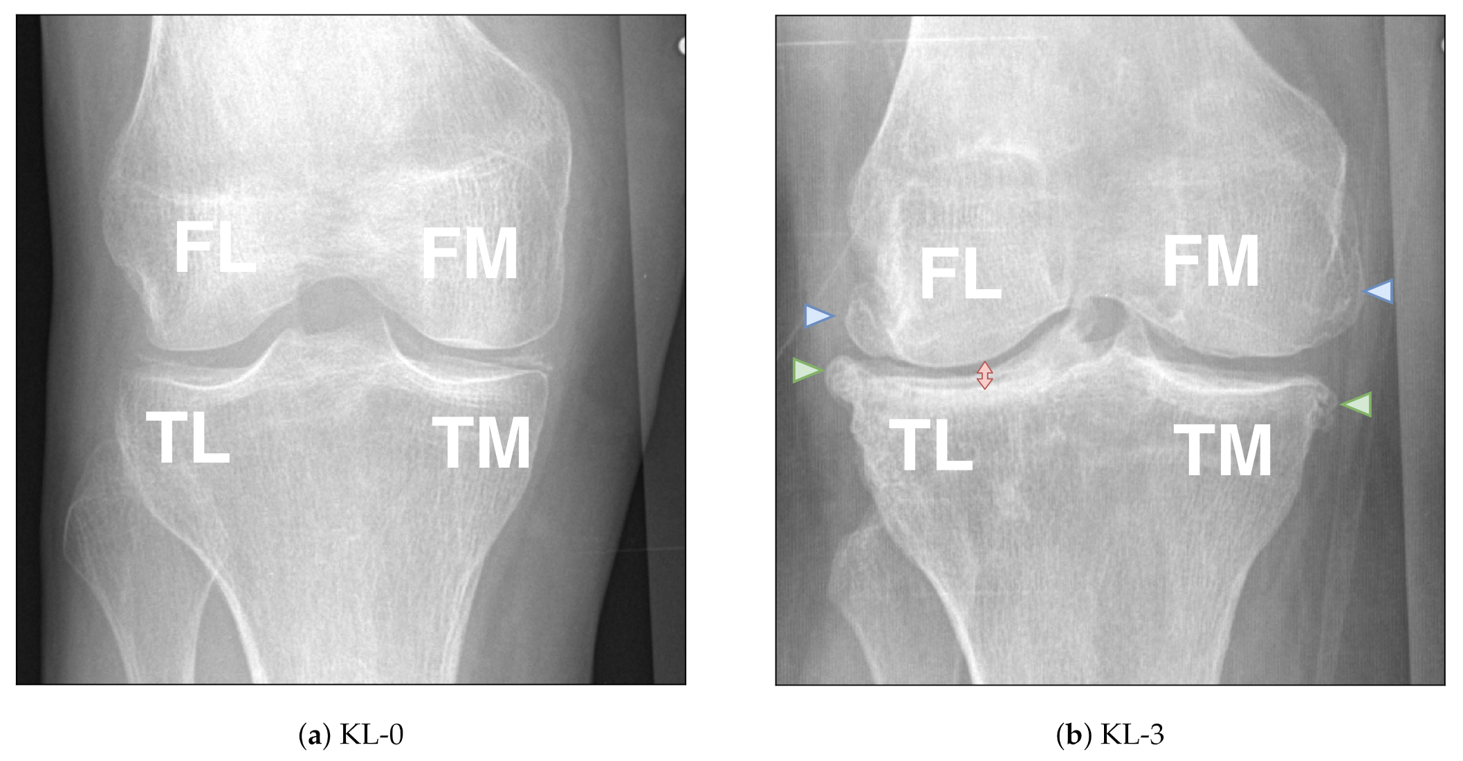
:1. Introduction
Contributions
- We demonstrate a possibility to accurately predict individual knee OA features and overall knee OA severity from plain radiographs simultaneously. Our method significantly outperforms previous state-of-the-art approach [15].
- Compared to the previous study [15], for the first time, we utilize two independent datasets for training and testing in assessing automatic OARSI grading: OAI and MOST, respectively.
- We perform an extensive experimental validation of the proposed methodology using various metrics and explore the influence of network’s depth, utilization of squeeze-excitation and ResNeXt blocks [16,17] on the performance, as well as ensembling, transfer learning and joint learning of KL and OARSI grading tasks.
- Finally, we also release the source codes and the pre-trained models allowing full reproducibility of our results.
2. Materials and Methods
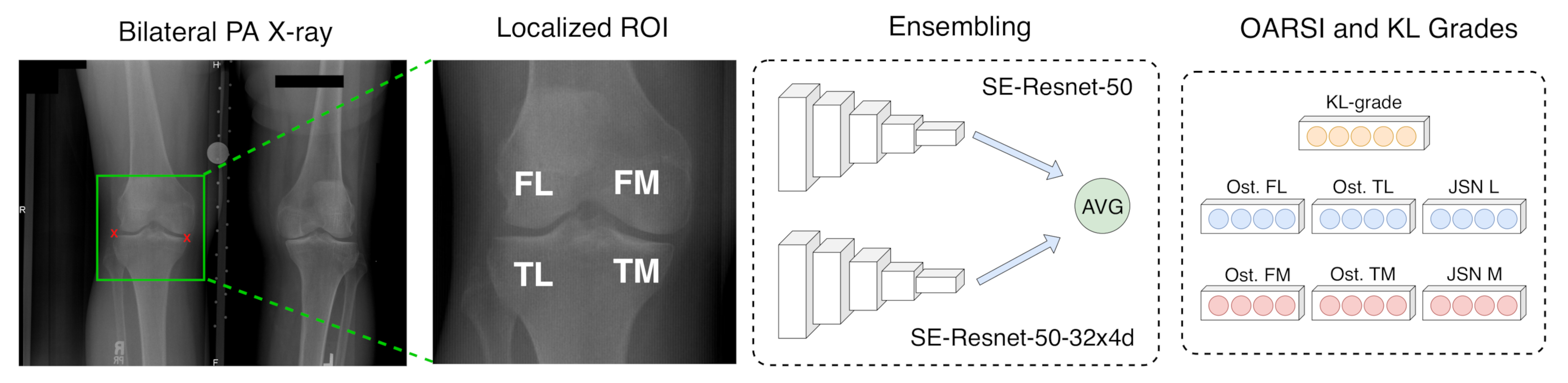
2.1. Overview
2.2. Data
2.3. Data Pre-Processing
2.4. Network Architecture
2.5. Training Strategy
3. Results
3.1. Cross-Validation Results and Backbone Selection
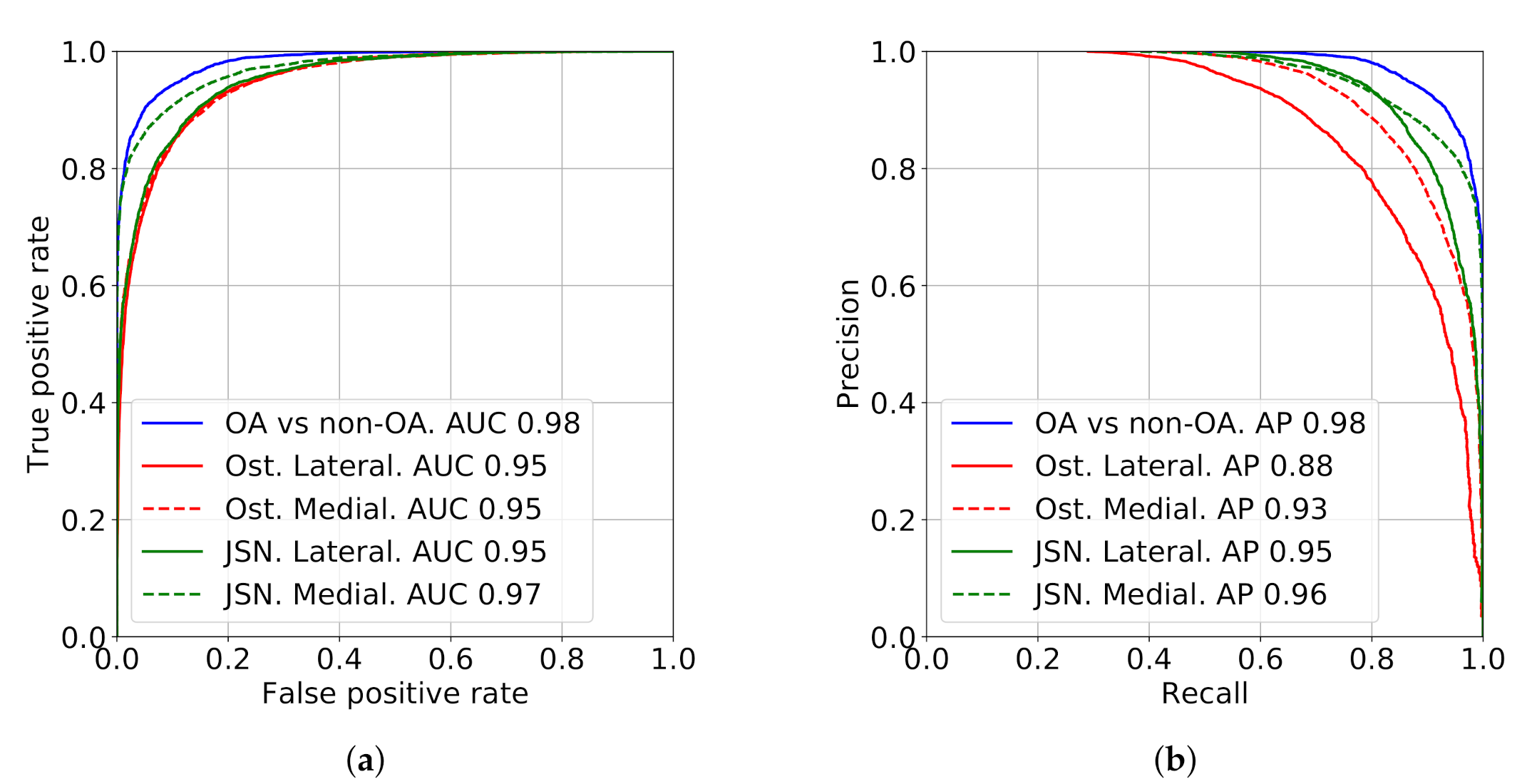
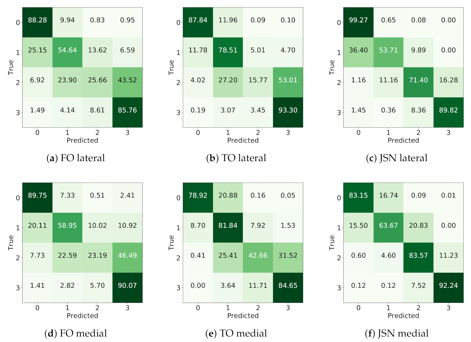
3.2. Test-Set Performance
3.3. Evaluation on the First Follow-Up of MOST Dataset
3.4. Evaluation of Performance with Respect to the Stage of OA
4. Discussion
Supplementary Materials
Author Contributions
Funding
Acknowledgments
Conflicts of Interest
Abbreviations
| OAI | Osteoarthritis Initiative |
| MOST | Multicenter Osteoarthritis Study |
| OA | Osteoarthritis |
| OARSI | Osteoarthritis Research Society International |
References
- Arden, N.; Nevitt, M.C. Osteoarthritis: Epidemiology. Best Pract. Res. Clin. Rheumatol. 2006, 20, 3–25. [Google Scholar] [PubMed]
- Cross, M.; Smith, E.; Hoy, D.; Nolte, S.; Ackerman, I.; Fransen, M.; Bridgett, L.; Williams, S.; Guillemin, F.; Hill, C.L.; et al. The global burden of hip and knee osteoarthritis: Estimates from the global burden of disease 2010 study. Ann. Rheum. Dis. 2014, 73, 1323–1330. [Google Scholar] [PubMed]
- Wluka, A.E.; Lombard, C.B.; Cicuttini, F.M. Tackling obesity in knee osteoarthritis. Nat. Rev. Rheumatol. 2013, 9, 225. [Google Scholar] [PubMed]
- Tiulpin, A.; Thevenot, J.; Rahtu, E.; Lehenkari, P.; Saarakkala, S. Automatic knee osteoarthritis diagnosis from plain radiographs: A deep learning-based approach. Sci. Rep. 2018, 8, 1727. [Google Scholar] [PubMed]
- Kellgren, J.; Lawrence, J. Radiological assessment of osteo-arthrosis. Ann. Rheum. Dis. 1957, 16, 494. [Google Scholar] [PubMed] [Green Version]
- Altman, R.D.; Gold, G. Atlas of individual radiographic features in osteoarthritis, revised. Osteoarthr. Cartil. 2007, 15, A1–A56. [Google Scholar]
- Esteva, A.; Robicquet, A.; Ramsundar, B.; Kuleshov, V.; DePristo, M.; Chou, K.; Cui, C.; Corrado, G.; Thrun, S.; Dean, J. A guide to deep learning in healthcare. Nat. Med. 2019, 25, 24. [Google Scholar]
- Pedoia, V.; Norman, B.; Mehany, S.N.; Bucknor, M.D.; Link, T.M.; Majumdar, S. 3D convolutional neural networks for detection and severity staging of meniscus and PFJ cartilage morphological degenerative changes in osteoarthritis and anterior cruciate ligament subjects. J. Magn. Reson. Imaging 2019, 49, 400–410. [Google Scholar]
- Norman, B.; Pedoia, V.; Majumdar, S. Use of 2D U-Net convolutional neural networks for automated cartilage and meniscus segmentation of knee MR imaging data to determine relaxometry and morphometry. Radiology 2018, 288, 177–185. [Google Scholar]
- Tiulpin, A.; Finnilä, M.; Lehenkari, P.; Nieminen, H.J.; Saarakkala, S. Deep-Learning for Tidemark Segmentation in Human Osteochondral Tissues Imaged with Micro-computed Tomography. arXiv 2019, arXiv:1907.05089. [Google Scholar]
- Tiulpin, A.; Klein, S.; Bierma-Zeinstra, S.; Thevenot, J.; Rahtu, E.; Van Meurs, J.; Oei, E.H.; Saarakkala, S. Multimodal Machine Learning-based Knee Osteoarthritis Progression Prediction from Plain Radiographs and Clinical Data. arXiv 2019, arXiv:1904.06236. [Google Scholar] [CrossRef] [PubMed]
- Antony, J.; McGuinness, K.; Moran, K.; O’Connor, N.E. Automatic detection of knee joints and quantification of knee osteoarthritis severity using convolutional neural networks. In Proceedings of the International Conference on Machine Learning and Data Mining in Pattern Recognition, Leipzig, Germany, 18–20 July 2007; Springer: Berlin/Heidelberg, Germany, 2017; pp. 376–390. [Google Scholar]
- Norman, B.; Pedoia, V.; Noworolski, A.; Link, T.M.; Majumdar, S. Applying Densely Connected Convolutional Neural Networks for Staging Osteoarthritis Severity from Plain Radiographs. J. Digit. Imaging 2018, 32, 471–477. [Google Scholar] [CrossRef] [PubMed]
- Xue, Y.; Zhang, R.; Deng, Y.; Chen, K.; Jiang, T. A preliminary examination of the diagnostic value of deep learning in hip osteoarthritis. PLoS ONE 2017, 12, e0178992. [Google Scholar] [CrossRef] [PubMed] [Green Version]
- Antony, A.J. Automatic Quantification of Radiographic Knee Osteoarthritis Severity and Associated Diagnostic Features Using Deep Convolutional Neural Networks. Ph.D. Thesis, Dublin City University, Dublin, Ireland, 2018. [Google Scholar]
- Hu, J.; Shen, L.; Sun, G. Squeeze-and-excitation networks. In Proceedings of the IEEE Conference on Computer Vision and Pattern Recognition, Salt Lake City, UT, USA, 18–22 June 2018; pp. 7132–7141. [Google Scholar]
- Xie, S.; Girshick, R.; Dollár, P.; Tu, Z.; He, K. Aggregated residual transformations for deep neural networks. In Proceedings of the IEEE Conference on Computer Vision and Pattern Recognition, Honolulu, HI, USA, 21–26 July 2017; pp. 1492–1500. [Google Scholar]
- Lindner, C.; Thiagarajah, S.; Wilkinson, J.M.; Wallis, G.A.; Cootes, T.F.; arcOGEN Consortium. Fully automatic segmentation of the proximal femur using random forest regression voting. IEEE Trans. Med. Imaging 2013, 32, 1462–1472. [Google Scholar] [CrossRef]
- Shin, H.C.; Roth, H.R.; Gao, M.; Lu, L.; Xu, Z.; Nogues, I.; Yao, J.; Mollura, D.; Summers, R.M. Deep convolutional neural networks for computer-aided detection: CNN architectures, dataset characteristics and transfer learning. IEEE Trans. Med. Imaging 2016, 35, 1285–1298. [Google Scholar] [CrossRef] [Green Version]
- Deng, J.; Dong, W.; Socher, R.; Li, L.J.; Li, K.; Fei-Fei, L. ImageNet: A Large-Scale Hierarchical Image Database. In Proceedings of the 2009 IEEE Conference on Computer Vision and Pattern Recognition, Miami, FL, USA, 20–25 June 2009. [Google Scholar]
- Kothari, M.; Guermazi, A.; Von Ingersleben, G.; Miaux, Y.; Sieffert, M.; Block, J.E.; Stevens, R.; Peterfy, C.G. Fixed-flexion radiography of the knee provides reproducible joint space width measurements in osteoarthritis. Eur. Radiol. 2004, 14, 1568–1573. [Google Scholar] [CrossRef]
- Tiulpin, A.; Thevenot, J.; Rahtu, E.; Saarakkala, S. A Novel Method for Automatic Localization of Joint Area on Knee Plain Radiographs. In Proceedings of the Scandinavian Conference on Image Analysis, Tromsø, Norway, 12–14 June 2017; Springer: Berlin/Heidelberg, Germany, 2017; pp. 290–301. [Google Scholar]
- He, K.; Zhang, X.; Ren, S.; Sun, J. Deep residual learning for image recognition. In Proceedings of the IEEE Conference on Computer Vision and Pattern Recognition, Las Vegas, NV, USA, 27–30 June 2016; pp. 770–778. [Google Scholar]
- Qiu, S. Global Weighted Average Pooling Bridges Pixel-level Localization and Image-level Classification. arXiv 2018, arXiv:1809.08264. [Google Scholar]
- Kingma, D.P.; Ba, J. Adam: A method for stochastic optimization. arXiv 2014, arXiv:1412.6980. [Google Scholar]
- Tiulpin, A. SOLT: Streaming over Lightweight Transformations. 2019. Available online: https://github.com/MIPT-Oulu/solt (accessed on 10 November 2020).
- Paszke, A.; Gross, S.; Chintala, S.; Chanan, G.; Yang, E.; DeVito, Z.; Lin, Z.; Desmaison, A.; Antiga, L.; Lerer, A. Automatic Differentiation in PyTorch. NIPS-W. 2017. Available online: https://openreview.net/forum?id=BJJsrmfCZ (accessed on 10 November 2020).
- Riddle, D.L.; Jiranek, W.A.; Hull, J.R. Validity and reliability of radiographic knee osteoarthritis measures by arthroplasty surgeons. Orthopedics 2013, 36, e25–e32. [Google Scholar] [CrossRef] [Green Version]
- Oka, H.; Muraki, S.; Akune, T.; Nakamura, K.; Kawaguchi, H.; Yoshimura, N. Normal and threshold values of radiographic parameters for knee osteoarthritis using a computer-assisted measuring system (KOACAD): The ROAD study. J. Orthop. Sci. 2010, 15, 781–789. [Google Scholar] [CrossRef]
- Thomson, J.; O’Neill, T.; Felson, D.; Cootes, T. Detecting Osteophytes in Radiographs of the Knee to Diagnose Osteoarthritis. In Proceedings of the International Workshop on Machine Learning in Medical Imaging, Athens, Greece, 17 October 2016; Springer: Berlin/Heidelberg, Germany, 2016; pp. 45–52. [Google Scholar]
- Antony, J.; McGuinness, K.; O’Connor, N.E.; Moran, K. Quantifying radiographic knee osteoarthritis severity using deep convolutional neural networks. In Proceedings of the 2016 23rd International Conference on Pattern Recognition (ICPR), Cancun, Mexico, 4–8 December 2016; pp. 1195–1200. [Google Scholar]
- Ching, T.; Himmelstein, D.S.; Beaulieu-Jones, B.K.; Kalinin, A.A.; Do, B.T.; Way, G.P.; Ferrero, E.; Agapow, P.M.; Zietz, M.; Hoffman, M.M.; et al. Opportunities and obstacles for deep learning in biology and medicine. J. R. Soc. Interface 2018, 15, 20170387. [Google Scholar] [CrossRef] [PubMed] [Green Version]
- Hinton, G.; Vinyals, O.; Dean, J. Distilling the knowledge in a neural network. arXiv 2015, arXiv:1503.02531. [Google Scholar]


| Dataset | # Images | Grade | # KL | # FO | # TO | # JSN | |||
|---|---|---|---|---|---|---|---|---|---|
| L | M | L | M | L | M | ||||
| OAI (Train) | 19704 | 0 | 2434 | 11,567 | 10,085 | 11,894 | 6960 | 17,044 | 9234 |
| 1 | 2632 | 4698 | 4453 | 5167 | 9181 | 1160 | 5765 | ||
| 2 | 8538 | 1748 | 2068 | 1169 | 2112 | 1061 | 3735 | ||
| 3 | 4698 | 1691 | 3098 | 1474 | 1451 | 439 | 970 | ||
| 4 | 1402 | - | - | - | - | - | - | ||
| MOST (Test) | 11743 | 0 | 4899 | 9008 | 7968 | 8596 | 6441 | 10,593 | 7418 |
| 1 | 1922 | 1336 | 1218 | 1978 | 3458 | 465 | 1865 | ||
| 2 | 1838 | 795 | 996 | 647 | 1212 | 442 | 1721 | ||
| 3 | 2087 | 604 | 1561 | 522 | 632 | 243 | 739 | ||
| 4 | 997 | - | - | - | - | - | - | ||
| Backbone | KL | FO | TO | JSN | |||
|---|---|---|---|---|---|---|---|
| L | M | L | M | L | M | ||
| Resnet-18 | 0.81 | 0.71 | 0.78 | 0.80 | 0.76 | 0.91 | 0.87 |
| Resnet-34 | 0.81 | 0.69 | 0.78 | 0.80 | 0.76 | 0.90 | 0.87 |
| Resnet-50 | 0.81 | 0.70 | 0.78 | 0.81 | 0.78 | 0.91 | 0.87 |
| SE-Resnet-50 | 0.81 | 0.71 | 0.79 | 0.81 | 0.78 | 0.91 | 0.87 |
| SE-ResNext50-32x4d | 0.81 | 0.72 | 0.79 | 0.82 | 0.78 | 0.91 | 0.87 |
| SE-Resnet-50 * | 0.78 | 0.66 | 0.73 | 0.76 | 0.70 | 0.91 | 0.87 |
| SE-ResNext50-32x4d * | 0.77 | 0.67 | 0.73 | 0.75 | 0.71 | 0.91 | 0.87 |
| SE-Resnet-50 ** | - | 0.71 | 0.79 | 0.82 | 0.78 | 0.91 | 0.88 |
| SE-ResNext50-32x4d ** | - | 0.73 | 0.80 | 0.83 | 0.78 | 0.91 | 0.88 |
| Ensemble | 0.82 | 0.73 | 0.80 | 0.83 | 0.79 | 0.92 | 0.88 |
| Side | Grade | A | K | MSE | ||
|---|---|---|---|---|---|---|
| L | FO | 0.69 (0.68–0.7) | 0.84 (0.84–0.85) | 0.22 (0.21–0.23) | 44.3 | 0.47 |
| TO | 0.64 (0.62–0.65) | 0.79 (0.78–0.8) | 0.33 (0.31–0.34) | 47.6 | 0.52 | |
| JSN | 0.79 (0.77–0.8) | 0.94 (0.93–0.95) | 0.04 (0.04–0.05) | 69.1 | 0.80 | |
| M | FO | 0.72 (0.71–0.73) | 0.83 (0.83–0.84) | 0.26 (0.25–0.27) | 45.8 | 0.48 |
| TO | 0.65 (0.64–0.67) | 0.84 (0.83–0.85) | 0.41 (0.38–0.44) | 47.9 | 0.61 | |
| JSN | 0.81 (0.8–0.82) | 0.9 (0.89–0.9) | 0.20 (0.19–0.20) | 73.4 | 0.75 | |
| Both | KL | 0.67 (0.66–0.67) | 0.82 (0.82–0.83) | 0.68 (0.65–0.70) | 63.6 | 0.69 |
| Stage | Side | Grade | F1 (weighted) | F1 (macro) | MSE | A | K |
|---|---|---|---|---|---|---|---|
| No | L | FO | 0.94 (0.93–0.94) | 0.36 (0.35–0.74) | 0.08 (0.07–0.09) | 0.85 (0.8–0.89) | 0.47 (0.42–0.53) |
| TO | 0.95 (0.94–0.95) | 0.31 (0.29–0.42) | 0.08 (0.07–0.1) | 0.74 (0.66–0.8) | 0.26 (0.19–0.32) | ||
| JSN | 0.99 (0.98–0.99) | 0.71 (0.62–0.8) | 0.01 (0.01–0.02) | 0.72 (0.61–0.84) | 0.42 (0.23–0.59) | ||
| M | FO | 0.85 (0.84–0.86) | 0.49 (0.48–0.5) | 0.17 (0.15–0.19) | 0.81 (0.78–0.83) | 0.49 (0.45–0.52) | |
| TO | 0.95 (0.95–0.96) | 0.34 (0.32–0.47) | 0.07 (0.06–0.09) | 0.79 (0.73–0.85) | 0.34 (0.26–0.41) | ||
| JSN | 0.86 (0.85–0.88) | 0.46 (0.45–0.48) | 0.16 (0.15–0.18) | 0.8 (0.76–0.83) | 0.45 (0.4–0.49) | ||
| Early | L | FO | 0.94 (0.93–0.94) | 0.36 (0.35–0.74) | 0.08 (0.07–0.09) | 0.85 (0.8–0.89) | 0.47 (0.42–0.53) |
| TO | 0.95 (0.94–0.95) | 0.31 (0.29–0.42) | 0.08 (0.07–0.1) | 0.74 (0.66–0.8) | 0.26 (0.19–0.32) | ||
| JSN | 0.99 (0.98–0.99) | 0.71 (0.62–0.8) | 0.01 (0.01–0.02) | 0.72 (0.61–0.84) | 0.42 (0.23–0.59) | ||
| M | FO | 0.85 (0.84–0.86) | 0.49 (0.48–0.5) | 0.17 (0.15–0.19) | 0.81 (0.78–0.83) | 0.49 (0.45–0.52) | |
| TO | 0.95 (0.95–0.96) | 0.34 (0.32–0.47) | 0.07 (0.06–0.09) | 0.79 (0.73–0.85) | 0.34 (0.26–0.41) | ||
| JSN | 0.86 (0.85–0.88) | 0.46 (0.45–0.48) | 0.16 (0.15–0.18) | 0.8 (0.76–0.83) | 0.45 (0.4–0.49) | ||
| Severe | L | FO | 0.66 (0.63–0.69) | 0.60 (0.57–0.63) | 0.48 (0.41–0.56) | 0.64 (0.61–0.67) | 0.81 (0.78–0.83) |
| TO | 0.64 (0.6–0.66) | 0.57 (0.54–0.6) | 0.77 (0.65–0.89) | 0.61 (0.57–0.64) | 0.74 (0.7–0.77) | ||
| JSN | 0.94 (0.93–0.95) | 0.66 (0.61–0.72) | 0.07 (0.05–0.08) | 0.68 (0.64–0.74) | 0.96 (0.95–0.97) | ||
| M | FO | 0.60 (0.57–0.63) | 0.6 (0.56–0.64) | 0.47 (0.42–0.52) | 0.62 (0.58–0.65) | 0.72 (0.69–0.75) | |
| TO | 0.64 (0.61–0.67) | 0.56 (0.52–0.59) | 0.85 (0.72–0.97) | 0.57 (0.53–0.61) | 0.66 (0.61–0.71) | ||
| JSN | 0.88 (0.86–0.9) | 0.70 (0.67–0.75) | 0.13 (0.11–0.16) | 0.73 (0.69–0.8) | 0.93 (0.92–0.94) |
Publisher’s Note: MDPI stays neutral with regard to jurisdictional claims in published maps and institutional affiliations. |
© 2020 by the authors. Licensee MDPI, Basel, Switzerland. This article is an open access article distributed under the terms and conditions of the Creative Commons Attribution (CC BY) license (http://creativecommons.org/licenses/by/4.0/).
Share and Cite
Tiulpin, A.; Saarakkala, S. Automatic Grading of Individual Knee Osteoarthritis Features in Plain Radiographs Using Deep Convolutional Neural Networks. Diagnostics 2020, 10, 932. https://doi.org/10.3390/diagnostics10110932
Tiulpin A, Saarakkala S. Automatic Grading of Individual Knee Osteoarthritis Features in Plain Radiographs Using Deep Convolutional Neural Networks. Diagnostics. 2020; 10(11):932. https://doi.org/10.3390/diagnostics10110932
Chicago/Turabian StyleTiulpin, Aleksei, and Simo Saarakkala. 2020. "Automatic Grading of Individual Knee Osteoarthritis Features in Plain Radiographs Using Deep Convolutional Neural Networks" Diagnostics 10, no. 11: 932. https://doi.org/10.3390/diagnostics10110932